Tracking. Readings: Chapter 17 of Forsyth and Ponce. Matlab Tutorials: motiontutorial.m. 2503: Tracking c D.J. Fleet & A.D. Jepson, 2009 Page: 1

Transcription

1 Goal: Tracking Fundamentals of model-based tracking with emphasis on probabilistic formulations. Examples include the Kalman filter for linear-gaussian problems, and maximum likelihood and particle filters for nonlinear/nongaussian problems. Outline Introduction Bayesian Filtering / Smoothing Likelihood Functions and Dynamical Models Kalman Filter Nonlinear/NonGaussian Processes Hill Climbing (Eigen-Tracking) Particle Filters Readings: Chapter 17 of Forsyth and Ponce. Matlab Tutorials: motiontutorial.m 2503: Tracking c D.J. Fleet & A.D. Jepson, 2009 Page: 1

2 Challenges in Tracking Tracking is the inference object shape, appearance, and motion as a function of time. Main players: what to model or estimate: shape (2D/3D), appearance, dynamics what to measure: color histograms, edges, feature points, flow,... Some of the main challenges: objects with many degrees of freedom, affecting shape, appearance, and motion; impoverished information due to occlusion or scale; multiple objects and background clutter

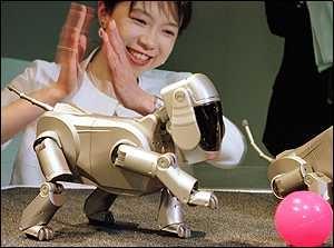
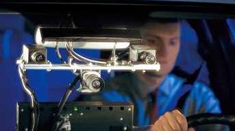
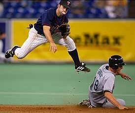
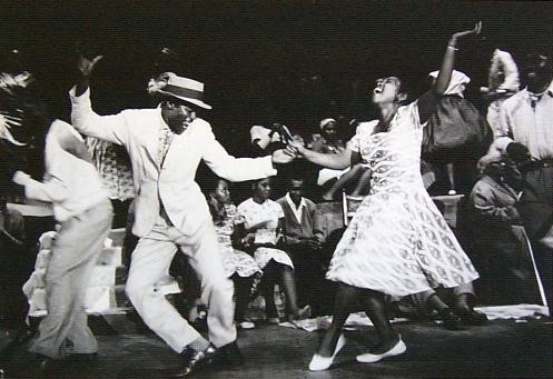
3 2503: Tracking space / aerospace surveillance smart toys automatic control sports / kinesiology human motion capture non-rigid motions biology (animal/cell/molecular) Page: 3

4 Probability and Random Variables A few basic properties of probability distributions will be used often: Conditioning (factorization): p(a, b) = p(a b) p(b) = p(b a) p(a) Bayes rule: p(a b) = p(b a) p(a) p(b) Independence: a and b are independent if and only if p(a, b) = p(a) p(b) Marginalization: p(b) = p(a, b) da, p(b) = a p(a, b) 2503: Tracking Notes: 4

5 Probabilistic Formulation We assume a state space representation in which time is discretized, and a state vector comprises all variables one wishes to estimate. State: denoted x t at time t, with the state history x 1:t = (x 1,..., x t ) continuous variables (position, velocity, shape, size,...) discrete variables (number of objects, gender, activity,...) Observations: the data measurements (images) with which we constrain state estimates, based on observation equation z t = f(x t ). The observations history is denoted z 1:t = (z 1,..., z t ) Posterior Distribution: the conditional probability distribution over states specifies all we can possibly know (according to the model) about the state history from the observations. p(x 1:t z 1:t ) (1) Filtering Distribution: often we only really want the marginal posterior distribution over the state at the current time given the observation history. This is called the filtering distribution: p(x t z 1:t ) = p(x 1:t z 1:t ) (2) x 1 x t 1 Likelihood and Prior: using Bayes rule we write the posterior in terms of a likelihood, p(z 1:t x 1:t ), and a prior, p(x 1:t ): p(x 1:t z 1:t ) = p(z 1:t x 1:t ) p(x 1:t ) p(z 1:t ) 2503: Tracking Page: 5

6 Model Simplifications The distribution p(x 1:t ), called a prior distribution, represents our prior beliefs about which state sequences (e.g., motions) are likely. First-order Markov model for temporal dependence (dynamics): p(x t x 1:t 1 ) = p(x t x t 1 ) (3) The order of a Markov model is the duration of temporal dependence (a first-order model requires past states up to a lag of one time step). With a first-order Markov model one can write the distribution over the state history as a product of transitions from one time to the next: p(x 1:t ) = p(x t x t 1 ) p(x 1:t 1 ) t = p(x 1 ) p(x j x j 1 ) (4) The distribution p(z 1:t x 1:t ), often called a likelihood function, represents the likelihood that the state generated the observed data. Conditional independence of observations: p(z 1:t x 1:t ) = p(z t x t ) p(z 1:t 1 x 1:t 1 ) t = p(z τ x τ ) (5) τ=1 That is, we assume that the observations at different times are independent when we know the true underlying states (or causes). 2503: Tracking Page: 6 j=2

7 Filtering and Prediction Distributions With the above model assumptions, one can express the posterior distribution recursively: p(x 1:t z 1:t ) p(z 1:t x 1:t ) p(x 1:t ) t t = p(z τ x τ ) p(x 1 ) p(x j x j 1 ) τ=1 j=2 p(z t x t ) p(x t x t 1 ) p(x 1:t 1 z 1:t 1 ) (6) The filtering distribution can also be written recursively: p(x t z 1:t ) = x 1 p(x 1:t z 1:t ) x t 1 = c p(z t x t ) p(x t z 1:t 1 ) (7) with a prediction distribution defined as p(x t z 1:t 1 ) = p(x t x t 1 ) p(x t 1 z 1:t 1 ) x t 1 (8) Recursion is important: it allows us to express the filtering distribution at time t in terms of the filtering distribution at time t 1 and the evidence at time t. all useful information from the past is summarized in the previous posterior (and hence in the prediction distribution). Without recursion one may have to store all previous images to compute the the filtering distribution at time t. 2503: Tracking Page: 7

8 Derivation of Filtering and Prediction Distributions Filtering Distribution: Given the model assumptions in Equations (4) and (5), along with Bayes rule, we can derive Equation (7) as follows: p(x t z 1:t ) = p(x 1:t z 1:t ) x 1 x t 1 1 = p(z 1:t x 1:t ) p(x 1:t ) p(z 1:t ) x 1 x t 1 = c p(z t x t ) p(z 1:t 1 x 1:t 1 ) p(x t x t 1 ) p(x 1:t 1 ) x 1 x t 1 = c p(z t x t ) p(x t x t 1 ) p(x 1:t 1, z 1:t 1 ) x 1 x t 1 = c p(z t x t ) p(x t x t 1 ) p(x 1:t 1, z 1:t 1 ) x t 1 x 1 x t 2 = c p(z t x t ) p(x t x t 1 ) p(x t 1, z 1:t 1 ) x t 1 = c p(z 1:t 1 ) p(z t x t ) p(x t x t 1 ) p(x t 1 z 1:t 1 ) x t 1 = c p(z t x t ) p(x t z 1:t 1 ). Batch Filter-Smoother (Forward-Backward Belief Propagation): We can derive the filtersmoother equation (9), for 1 < τ t, as follows: 1 p(x τ z 1:t ) = p(x 1:t ) p(z 1:t x 1:t ) p(z 1:t ) x 1:τ 1 x τ+1:t = c p(x 1:τ ) p(x τ+1:t x τ ) p(z 1:τ 1 x 1:τ 1 ) p(z τ x τ ) p(z τ+1:t x τ+1:t ) x 1:τ 1 x τ+1:t = c p(z τ x τ ) p(x 1:τ ) p(z 1:τ 1 x 1:τ 1 ) p(x τ+1:t x τ ) p(z τ+1:t x τ+1:t ) x 1:τ 1 x τ+1:t = c p(z τ x τ ) p(x τ z 1:τ 1 ) p(x τ x τ+1:t ) p(x τ+1:t) p(x τ+1:t z τ+1:t ) p(z τ+1:t) x τ+1:t p(x τ ) p(x τ+1:t ) = c p(z τ x τ ) p(x τ z 1:τ 1 ) p(z τ+1:t) p(x τ x τ+1:t ) p(x τ+1:t z τ+1:t ) p(x τ ) x τ+1:t c = p(x τ ) p(z τ x τ ) p(x τ z 1:τ 1 ) p(x τ z τ+1:t ). 2503: Tracking Notes: 8

9 Filtering and Smoothing Provided one can invert the dynamics equation, one can also perform inference (recursively) backwards in time: p(x τ z τ:t ) = c p(z τ x τ ) p(x τ x τ+1 ) p(x τ+1 z τ+1:t ) x τ+1 = c p(z τ x τ ) p(x τ z τ+1:t ) That is, the distribution depends on the likelihood the current data, the inverse dynamics, and the filtering distribution at time t + 1. Smoothing distribution (forward-backward belief propagation): p(x τ z 1:t ) = c p(x τ ) p(z τ x τ ) p(x τ z 1:τ 1 ) p(x τ z τ+1:t ) (9) The smoothing distribution therefore accumulates information from past, present, and future data. Batch Algorithms: Estimation of state sequences using the entire observation sequence (i.e., using all past, present & future data): the filter-smoother algorithm is efficient, when applicable. storage/delays make this unsuitable for many tracking domains. Online Algorithms: Recursive inference (7) is causal. Estimation of x t occurs as soon as observations at time t are available, thereby using present and past data only. 2503: Tracking Page: 9

10 Likelihood Functions There are myriad ways in which image measurements have been used for tracking. Some of the most common include: Feature points: E.g., Gaussian noise in the measured feature point locations. The points might be specified a priori, or learned when the object is first imaged at time 0. Image templates: E.g., subspace models learned prior to tracking, or brightness constancy as used in flow estimation. Color histograms: E.g., mean-shift to track modes of local color distribution, for robustness to deformations. Gradient histograms: E.g., histograms of oriented gradients (HOG) in local patches to capture image orientation structure as a function of spatial position over target. Image curves (or edges): E.g., with Gaussian noise in measured location normal to the contour. 2503: Tracking Page: 10

11 Temporal Dynamics We often assume a combination of deterministic and stochastic dynamics. Common linear models include: Random walk with zero velocity and IID Gaussian process noise: x t = x t 1 + η d, η d N(0, C) Random walk with zero acceleration and Gaussian process noise ( ) ( ) ( ) ( ) xt 1 1 xt 1 ηd = + v t 0 1 v t 1 ǫ d where η d N(0, C x ) and ǫ d N(0, C v ). For higher-order models we define an augmented state vector, and then use a first-order formulation. E.g., for a second-order model: x t = Ax t 1 + Bx t 2 + η d one can define y t ( xt x t 1 ) for which the equivalent first-order augmented-state model is ( ) ( ) A B ηd y t = y t 1 + I 0 0 Typical observation model: z t =f( [I 0] y t ) plus Gaussian noise. 2503: Tracking Page: 11

12 Dynamical Models There are many other useful dynamical models. For example, harmonic oscillation can be expressed as or as a first order system with d u dt = d 2 x dt 2 ( ) 0 1 u, 1 0 = x ( ) x where u v A first-order approximation yields: ( ) u t = u t 1 + t d u dt + η ǫ ( ) ( ) 1 t η = u t 1 + t 1 ǫ In many cases it is useful to learn a suitable model of state dynamics. There are well-know algorithms for learning linear auto-regressive models of variable order. 2503: Tracking Notes: 12

13 Kalman Filter Assume a linear dynamical model with Gaussian process noise, and a linear observation model with Gaussian observation noise: x t = A x t 1 + η d, η d N(0, C d ). (10) z t = M x t + η m, η m N(0, C m ) (11) The transition density is therefore Gaussian, centred at mean A x t 1, with covariance C d : p(x t x t 1 ) = G(x t ; A x t 1, C d ). (12) The observation density is also Gaussian: p(z t x t ) = G(z t ; M x t, C m ). (13) Because the product of Gaussians is Gaussian, and the marginals of a Gaussian are Gaussian, it is straightforward (but tedious) to show that the prediction and filtering distributions are both Gaussian: p(x t z 1:t 1 ) = p(x t x t 1 ) p(x t 1 z 1:t 1 ) = G(x t ; x t, C t ) (14) x t 1 p(x t z 1:t ) = cp(z t x t ) p(x t z 1:t 1 ) = G(x t ; x + t, C+ t ) (15) with closed-form expressions for the means x t, x + t and covariances Ct, C t : Tracking Page: 13

14 Kalman Filter Depiction of Kalman updates: deterministic drift posterior at t-1 data incorporate data stochastic diffusion posterior at t prediction at t 2503: Tracking Page: 14

15 Kalman Filter (details) To begin, suppose we know that x N( 0, C), and let y = Ax. Since x is zero-mean, it is clear that y will also be zero-mean. Further, the covariance of y is given by E[ y y T ] = E[ A xx T A T ] = A E[ xx T ] A T = A C A T (16) Now, let s use this to derive the form of the prediction distribution. Let s say that we know the filtering distribution from the previous time instant, t 1, and let s say it is Gaussian with mean x + t 1 with covariance C t 1. + p(x t 1 z 1:t 1 ) = G(x t 1 ; x + t 1, C+ t 1 ). (17) And, as above, we assume a linear-gaussian dynamical model, x t = A x t 1 + η d, η d N(0, C d ). (18) From above we know that A x t 1 is Gaussian. And we ll assume that the Gaussian process noise η d is independent of the previous posterior distribution. So, 18 is the sum of two independent Gaussian random variable, and hence the corresponding density is just the convolution of their individual densities. Remember that the convolution of two Gaussians with covariances C 1 and C 2 is Gaussian with covariance C 1 + C 2. With this, it follows from (17) and (18) that the prediction mean and covariance of p(x t z 1:t 1 ) in (14) are given by x t = A x + t 1, C t = A C + t 1 AT + C d. This gives us the form of the prediction density. Now, let s turn to the filtering distribution. That is, we wish to combine the prediction distribution with the observation density for the current observation, z t, in order to form the filtering distribution at time t. In particular, using (15), with (13) and the results above, it is straightforward to see that p(x t z 1:t ) p(z t x t ) p(x t z 1:t 1 ) (19) = G(z t ; Mx t, C m ) G(x t ; x t, C t ). (20) Of course the product of two Gaussians is Gaussian; and it remains to work out expressions for its mean and covariance. This requires somewhat tedious algebraic manipulation.

16 While there are many ways to express the posterior mean and covariance, the conventional solution defines an intermediate quantity called the Kalman Gain, K t, given by K t = C ( ) t 1 MT MCt 1 1 MT + C m. Using the Kalman gain, one can express the posterior mean and variance, x + t and C t +, as follows: x + t = x t + K t ( zt Mx t ), C + t = (I K t M) C t = (I K t )C t (I K t) T + K t C m K T t The Kalman filter began to appear in computer vision papers in the late 1980s. The first two main applications were for (1) automated road following where lane markers on the highway were tracking to keep a car on the road; and (2) the estimation of the 3D struction and motion of a rigid object (or scene) with respect to a camera, given a sequences of point tracks through time. Dickmanns & Graefe, Dynamic monocular machine vision. Machine Vision and Appl., Broida, Chandrashekhar & Chellappa, Rigid structure from feature tracks under perspective projection. IEEE Trans. Aerosp. & Elec. Sys., R.E. Kalman 2503: Tracking Notes: 16

17 Non-linear / Non-Gaussian Systems Tracking problems are rarely linear/gaussian. The posterior, filtering and prediction distributions are usually nongaussian, and often they are multimodal. The reasons for this include, among other things, scene clutter and occlusion, where many parts of the scene may appear similar to parts of the object being tracking image observation models are often nonlinear with heavy-tailed noise so that we can cope with outliers, complex appearance changes, and the nonlinearity of perspective projection. temporal dynamics are often nonlinear (e.g., human motion) For example: Background clutter and distractors. Nonlinear dynamics. 2503: Tracking Page: 17

18 Extended and Unscented Kalman Filters Extended Kalman Filter (EKF): For nonlinear dynamical models one can linearize the dynamics at current state; that is, x t = f( x t 1 ) + η d A x t 1 + η d, where A = f( x) x= xt 1 and η d N(0, C d ). One can also iterate the approximation to obtain the Iterated Extended Kalman Filter (IEKF). In practice the EKF and IEKF have problems unless the dynamics are close to linear. Unscented Kalman Filter (UKF): Estimate posterior mean and variance to second-order with arbitrary dynamics [Julier & Uhlmann, 2004]. Rather than linearize the dynamics to ensure Gaussian predictions, use exact 1 st and 2 nd moments of the prediction density under the nonlinear dynamics: Choose sigma points x j whose sample mean and covariance equal the mean and variance of the Gaussian posterior at t Apply nonlinear dynamics to each sigma point, y j = f(x j ), and then compute the sample mean and covariances of the y j. Monte Carlo sampling Linear Approx (EKF) Unscented Transform 2503: Tracking Notes: 18

19 Hill-Climbing Rather than approximating the posterior or filtering distributions (fully), just find local maxima of the filtering distribution at each time step. By also computing the curvature of the log filtering distribution at the maxima, one obtains local Gaussian approximations. E.g., Eigen-Tracking [Black & Jepson, 96]: Assume we have learned (offline) a subspace appearance model for an object under varying pose, articulation, and lighting: B(x, c) = k c k B k (x) During tracking, we seek the image warp parameters a t, at each time t, and the subspace coefficients c t such that the warped image is explained by the subspace; i.e., I(w(x, a t ), t) B(x, c t ) A robust objective function helps cope with modeling errors, occlusions and other outliers: E(a t, c t ) = x ρ( I(w(x, a t ), t) B(x, c t ) ) Initialize the estimation at time t with ML estimate from time t : Tracking Page: 19

20 Eigen-Tracking Image sequence Training eigenimages training images Warp Reconstruct Test Results: Figures show superimposed tracking region (top), the best reconstructed pose (bottom left), and the closest training image (bottom right). 2503: Tracking Page: 20

21 Sequential Monte Carlo For many problems ambiguity is sufficiently problematic that we must maintain a better representation of the filtering distribution. Approximate the filtering distribution, p(x t z 1:t ), using a weighted sample set, S = {x (j) t, w (j) t }; i.e., with a collection of point probability masses at locations x (j) t weight function w(x). with weights w (j) t = w(x (j) t ) for some Let s consider this in more detail below. Monte Carlo: Approximate the filtering distribution P with samples drawn from it, S = {x (j) } N j=1. Then, use sample statistics to approximate expectations under P; i.e., for functions f(x), E S [f(x) ] 1 N N j=1 f(x (j) ) N f(x) P(x) dx E P [ f(x) ] But, we don t know how to draw samples from our distribution p(x t z 1:t ). 2503: Tracking Page: 21

22 Importance Sampling: Particle Filter If one draws samples x (j) from a proposal distribution, Q(x), with weights w (j), then N E S [f(x) ] w (j) f(x (j) ) N E Q [ w(x) f(x) ] j=1 If w(x) = P(x)/Q(x), then the weighted sample statistics approximate the desired expectations under P(x); i.e., E Q [w(x) f(x) ] = w(x) f(x) Q(x) dx = f(x) P(x) dx = E P [ f(x) ] Sequential Monte Carlo [Arulampalam et al, 2002]: The sample set is updated each time instant, incorporating new data, and possibly re-sampling the set of state samples x (j). Key idea: exploit the form of the filtering distribution for importance sampling, p(x t z 1:t ) = c p(z t x t ) p(x t z 1:t 1 ) and the facts that it is often easy to evaluate the likelihood, and one can usually draw samples from the prediction distribution Simple Particle Filter: If we sample from the prediction distribution Q = p(x t z 1:t 1 ) then the weights must be w(x) = cp(z t x t ), with c = 1/p(z t z 1:t 1 ). 2503: Tracking Page: 22

23 Simple Particle Filter Step 1: Sample the approximate filtering distribution, p(x t 1 z 1:t 1 ), given the weighted sample set S t 1 = {x (j) t 1, w(j) t 1 }. To do this, treat the N weights as probabilities and sample from the cumulative weight distribution; i.e., draw sample u U(0, 1) to sample an index i. 1 u 0 0 i N Step 2: With sample x (i) t 1, the dynamics provides a distribution over states at time t, i.e., p(x t x (i) t 1 ). A fair sample from the dynamics, x (j) t p(x t x (i) t 1 ) is then a fair sample from the prediction distribution p(x t z 1:t 1 ). Step 3: To complete one iteration to find the new filtering distribution, given the samples x (j) t, we compute the weights w (j) t = c p(z t x (j) t ): p(z t x (j) t ) is the data likelihood that we know how to evaluate. Using Bayes rule one can show that c satisfies 1 c = p(z t z 1:t 1 ) = p(z t x t ) p(x t z 1:t 1 ) dx t p(z t x (j) t ) j Using the approximation, the weights become normalized likelihoods (so they sum to 1). 2503: Tracking Page: 23

24 Particle Filter Remarks One can think of a sampled approximation as a sum of Dirac delta functions. A weighted sample set S t 1 = {x (j) t 1, w t 1}, (j) is just a weighted set of delta functions:: p(x t 1 z 1:t 1 ) = N j=1 w (j) δ(x t 1 x (j) t 1) Sometimes people smooth the delta functions to create smoothed approximations (called Parzen window density estimates). If one considers the prediction distribution, and uses the properties of delta functions under integration, then one obtains a mixture model for the prediction distribution. That is, given a weighted sample set S t 1 as above the prediction distribution in (8) is a linear mixture model p(x t z 1:t 1 ) = N j=1 w (j) p(x t x (j) t 1) The sampling method on the previous page is just a fair sampling method for linear mixture models. For more background on particle filters see papers by Gordon et al (1998), Isard and Blake (IJCV, 1998), and by Fearnhead (Phd) and Liu and Chen (JASA, 1998). 2503: Tracking Notes: 24

25 Particle Filter Steps Summary of main steps in basic particle filter: sample sample normalize p(x t 1 z 1:t 1 ) p(x t x t 1 ) p(z t x t ) p(x t z 1:t ) filtering temporal likelihood filtering distribution dynamics evaluation distribution Depiction of the particle filter process (after [Isard and Blake, 98]): weighted sample set re-sample and drift diffuse and re-sample compute likelihoods weighted sample set 2503: Tracking Page: 25

26 Particle Filter Example State: 6 DOF affine motion Measurement: edge locations normal to contour Dynamics: second-order Markov Computation: 1000 particles with re-sampling every frame [Isard and Blake, 98] Depiction of the filtering distribution evolving through time. 2503: Tracking Page: 26

27 Particle Explosion in High Dimensions The number of samples N required by our simple particle filter depends on the effective volumes (entropies) of the prediction and posterior distributions. With random sampling from the prediction density, N must grow exponentially in state dimension D if we expect enough samples to fall on states with high posterior probability. Prediction Posterior E.g., for D-dimensional spheres, with radii R and r, N ( ) R D r 2503: Tracking Page: 27

28 Example: 3D People Tracking Goal: Estimate human pose and motion from monocular video. Model State: 3D kinematic tree with 6 global degrees of freedom and 22 joint angles right elbow right hand right shoulder right knee right hip right ear upper back top of head lower back right heel left ear left hip left knee left shoulder left elbow left hand Likelihood & Dynamics: Given the state, s, and camera model, 3D marker positions X j project onto the 2D image plane to locations left heel Observation model: d j (s) = T(X j ; s). ˆd j = d j + η j, η j N(0, σ 2 mi 2 ). Likelihood of observed 2D locations, D = {ˆd j }: p(d s) exp( 1 ˆd 2σm 2 j d j (s) 2 ). Smooth dynamics: s t = s t 1 + ǫ t. where ǫ t is isotropic Gaussian for translational and angular variables. j 2503: Tracking Page: 28

29 Example: 3D People Tracking (cont) Estimator Variance: expected squared error (from posterior mean), computed over multiple runs with independent noise. With N fair posterior samples the estimator variance will decrease like 1/N Full Body Tracker (right hip) Hybrid Monte Carlo Particle Filter Var[ mean right hip, β ] Computation Time (particle filter samples) The estimator variance does not decrease anything like 1/N. Better samplers are necessary. E.g., Hybrid Monte Carlo Filter [Choo & Fleet 01]: A particle filter with Markov chain Monte Carlo updates is more efficient. Particle Filter HMC Filter (black: ground truth; red: mean states from 6 trials) 2503: Tracking Page: 29

30 Effective Sample Size If we drew N fair samples from the posterior, then estimator variance decreases like 1/N. We can approximate the number of independent samples (called the effective sample size) as follows: N e 1 j (w(j) ) 2 In the worst case, when only one weight is significantly non-zero, N e is close to one. In the best case, with N fair samples, all weights are 1/N so N e =N. In practice, when N e is large (e.g., > 100, but this depends on the task), one should not necessarily re-sample the posterior. You may just propagate each sample forward by sampling from the transition density. when N e is small (e.g., < 10), you likely have an unreliable posterior approximation, and you may lose track of the target. You need more or better samples! 2503: Tracking Page: 30

31 Residual Sampling Given N samples {x k } N k=1 with weights {w k} N k=1, where k w k = 1, and assume that we wish to draw N new samples (with replacement). Rather than treating the weights are probabilities of a multinomial distribution and drawing N independent samples, one can greatly reduce sampling variability by using residual sampling. The expected number of times we expect to draw x k is n k = Nw k. So first place n k copies of x k in the new sample set, and let the residual weights be a k = n k n k. Then, draw N k n k samples (with replacement) according to the probabilities p k = a k / k a k. 2503: Tracking Notes: 31

32 Use the Current Observation to Improve Proposals The proposal distribution Q should be as close as possible to the filtering distribution P that we wish to approximate. Otherwise, many particles will have weights near zero, contributing very little to the approximation to the filtering disitribution; we may even fail to sample significant regions of the state space, so the normalization constant c can be wildly wrong. For visual tracking, the prediction distribution Q = p(x t z 1:t 1 ) often yields very poor proposals, because dynamics are often very uncertain, and likelihoods are often very peaked by comparison. One way to greatly improve proposals is to use the current observation. For example, imagine that you are tracking faces and you have a low-level face detector. Let D(x t ) be a continuous distribution obtained from some low-level detector which indicates where faces might be (e.g., Gaussian modes at locations of classifier hits). Then, just modify the proposal density and importance weights: Q(x t ) = D(x t ) p(x t z 1:t 1 ), with w(x t ) = c p(z t x t ) D(x t ) 2503: Tracking Notes: 32

33 Explain All Observations Don t compare different states based on different sets of observations. If one hypothesizes two target locations, s 1 and s 2, and extracts target-sized image regions centered at both locations, I 1 and I 2, it makes no sense to say s 1 is more likely if p(i 1 s 1 ) > p(i 2 s 2 ). Rather, use p(i s 1 ) and p(i s 2 ) where I is the entire image. Explain the entire image, or use likelihood ratios (for efficiency). E.g., assume that pixels I(y), given the state, are independent, so p(i x) = y D f p f (I(y) s) y D b p b (I(y)) where D f and D b are disjoint sets of foreground and background pixels, and p f and p b are the respective likelihood functions. Divide p(i s) by the background likelihood of all pixels (i.e., as if no target is present): y D p(i s) f p f (I(y) s) y D b p b (I(y)) y p b(i(y)) y D = f p f (I(y) s) y D b p b (I(y)) y D f p b (I(y) s) y D b p b (I(y)) = p f (I(y) x) p b (I(y)) y D f 2503: Tracking Notes: 33

34 Conditional Observation Independence What about independence of measurements? Pixels have correlated (dependent) noise because of several factors: models are wrong (most noise is model error) failures in feature tracking are not independent for different features. overlapping windows are often used to extract measurements Consequence: Likelihood functions are often more sharply peaked than they ought to be. 2503: Tracking Notes: 34

35 Summary and Further Remarks on Filtering posteriors must be sufficiently constrained, with some combinations of posterior factorization, dynamics, measurements,.. proposal distributions should be non-zero wherever the posterior distribution is non-zero (usually heavy-tailed) proposals should exploit current observations in addition to prediction distribution likelihoods should be compared against the same observations sampling variability can be a problem must have enough samples in regions of high probability for normalization to be useful too many samples needed for high dimensional problems (esp. when samples drawn independently from prediction dist) samples tend to migrate to a single mode (don t design a particle filter to track multiple objects with a state that represents only one such object) sample deterministically where possible exploit diagnostics to monitor effective numbers of samples 2503: Tracking Page: 35

36 Further Readings Arulampalam, M.S., Maskell, S., Gordon, N. and Clapp, T. (2002) A tutorial on particle filters for online nonlinear/non-gaussian Bayesian tracking. IEEE Trans. Signal Proc. 50(2): Black, M.J. and Jepson, A.D. (1996) Eigentracking: Robust matching and tracking of articulated objects using a view-based representation. Int. J. Computer Vision, 26: Blake, A. (2005) Visual tracking. In Mathematical models for Computer Vision: The Handbook. N. Paragios, Y. Chen, and O. Faugeras (eds.), Springer, Carpenter, Clifford and Fearnhead (1999) An improved particle filter for nonlinear problems. IEE Proc. Radar Sonar Navig., 146(1) Doucet, A., Godsill, S., and Andrieu, C. (2000) On sequential Monte Carlo sampling methods for Bayesian filtering. Stats and Computing, 10: Gordon, N.J., Salmond, D.J. and Smith, A.F.M. (1993) Novel approach to nonlinear/non-gaussian Bayesian state estimation. IEE Proceedings-F, 140(2): Isard, M. and Blake, A. (1998) Condensation: Conditional density propagation. Int. J. Computer Vision, 29(1):2 28. Jepson, A.D., Fleet, D.J. and El-Maraghi, T. (2003) Robust, on-line appearance models for visual tracking. IEEE Trans. on PAMI, 25(10): Julier, S.J. and Uhlmann, J.K. (2004) Unscented filtering and nonlinear estimation. Proceedings of the IEEE, 92(3): Khan, Z., Balch, T. and Dellaert, F. (2004) A Rao-Blackwellized particle filter for EigenTracking. Proc. IEEE CVPR. Sidenbladh, H., Black, M.J. and Fleet, D.J. (2000) Stochastic tracking of 3D human figures using 2D image motion. Proc. ECCV, pp , Dublin, Springer. Wan, E.A. and van der Merwe, R. (2000) The unscented Kalman filter for nonlinear estimation. (see van der Merwe s web site for the TR) 2503: Tracking Notes: 36