Darwin Uy Math 538 Quiz 4 Dr. Behseta

Size: px

Start display at page:

Download "Darwin Uy Math 538 Quiz 4 Dr. Behseta"

Victor Morgan
6 years ago
Views:

1 Darwin Uy Math 538 Quiz 4 Dr. Behseta 1) Section talks about how when sample size gets large, posterior distributions become approximately normal and centered at the MLE. This is largely due to Taylor s theorem. We first note that the Taylor expansion of the likelihood around our MLE estimate of θ, θ, is equal to l(θ) = l θ + l θ θ θ θ θ t H l θ θ θ Noticing that l θ is a constant and that l θ = 0, we get l(θ) = C θ θ t H l θ θ θ As n gets large is that the prior distribution contributes a negligible amount to the posterior; the likelihood approaches the form of the normal distribution and the prior b fixed as n increases. This is because as n gets larges the standard error of θ drops and which will cause θ θ to be small. Since this difference is small, our posterior distribution is approximately constant, π(θ) π θ. Also when n gets large, only values of θ such that θ θ is small give appreciable posterior probability. We therefore end up with an approximation for our posterior to be f(θ y) exp 1 2 θ θ t H θ θ θ, This is the kernel of a multivariate normal distribution with mean equal to the θ, and variance equal to the negative inverse of the observed information,- H 1 θ. This gives a convenient way to compute posteriors for large samples as well as shows us that with enough data, different beliefs will eventually come to an agreement. 2) Bayesian inference are great for neural data because : 1) Inferences agree reasonably well with those obtained from ML estimation 2) We can sometimes use the prior to formalize structure in the data 3) There are general computational tools to compute posteriors in many complicated statistical models

2 When we have conjugate priors, posterior probabilities can be easily calculated. This unfortunately is not always the case. When the posterior takes a form that is not easily recognizable, we run into numerical problems, such integration to find probabilities. This problem can be solved by doing posterior simulation based off of Markov Chain Monte Carlo (MCMC). We first suppose that the state at time t+1 is dependent on only the state at time t, and independent of the states before t. We also suppose that these conditional probabilities are time invariant. Then if the chain is irreducible, aperiodic, and recurrent we can say that the long term behavior of the chain will eventually hit a limiting distribution. This distribution is known as the stationary distribution and once it is reached the chain will stay there. This is important for the posterior simulation because we believe that once a chain runs for a period of time and hits the stationary distribution which we design to be the posterior distribution, we begin to simulate from the posterior distribution. The most common MCMC algorithm is known as the Metropolis-Hastings algorithm. In theory the MH algorithm works because it will eventually hit the stationary distribution. The period before the convergence of the distribution is known as the burn in period. The length of the burn is dependent on the jumping density. Ideally we can use the proposal density/ jumping density as the posterior pdf, but we really choose the jumping by its simplicity to simulate. 11.2) library("mvtnorm", lib.loc="c:/program Files/R/R /library") data=matrix(c(-.86, -.30, -.05,.73,5,5,5,5, 0,1,3,5),nrow=4,ncol=3) summary(glm(cbind(data[,3],data[,2]-data[,3])~data[,1],family=binomial(link = "logit"))) Jsig=diag(c(1^2,4^2)) sim=matrix(c( ,5.7488),nrow=1, ncol=2) for (i in 1:100000) { prop=sim[i,]+rmvnorm(1,c(0,0),jsig) r=min(1,( prod(dbinom(data[,3],5, exp(prop[1]+prop[2]*data[,1])/(1+exp(prop[1]+prop[2]*data[,1])) ))/prod(dbinom(data[,3],5, exp(sim[i,1]+sim[i,2]*data[,1])/(1+exp(sim[i,1]+sim[i,2]*data[,1])) )) )) r[is.nan(r)]=0 if (runif(1)<r) {sim=rbind(sim,prop) else sim=rbind(sim,sim[i,]) plot (sim[50000:100000,1],sim[50000:100000,2], xlim=c(-4,10),ylim=c(-10,40)) hist(sim[50000:100000,1]) hist(sim[50000:100000,2]) hdr1 <- hdr.2d(sim[50000:100000,1],sim[50000:100000,2]) plot(hdr1, pointcol="red", show.points=true, pch=3, xlab="sweat rate", ylab="sodium")

3 For this simulation we chose our starting point to be α = β = These are our least-squares estimates obtained from the GLM. We then define our jumping distribution to be the multivariate normal distribution centered at 0. We did 100,000 simulation with a 50,000 burn in period. Our simulation yields the results We can say with 95% probability that < α <

We can say with 95% probability that 3.478413 < β < 24.947228.

4 We can say with 95% probability that < β < Our results are fairly similar to the results yielded in the book.

5 3) library("mvtnorm", lib.loc="c:/program Files/R/R /library") library("bayesm", lib.loc="c:/program Files/R/R /library") #data reading=matrix(c( 59, 77, 43, 39, 34, 46, 32, 26, 42, 38, 38, 43, 55, 68, 67, 86, 64, 77, 45, 60, 49, 50, 72, 59, 34, 38, 70, 48, 34, 55, 50, 58, 41, 54, 52, 60, 60, 75, 34, 47, 28,48, 35, 33),nrow=22,ncol=2,byrow=T) #prior parameters Sig0=matrix(c(625, 312.5, 312.5, 625),nrow=2, ncol=2) mu0=c(50,50) sigma=matrix(0,nrow=2, ncol=2) propsigma=matrix(0,nrow=2, ncol=2) sim=matrix(c(50,50, 625, 312.5,625 ), nrow=1, ncol=5) for (i in 1:100000) { sigma=matrix(0,nrow=2, ncol=2) mu=sim[i, 1:2] for (ii in 1:2) { for (j in ii:2) {sigma[ii,j]= sim[i,1+ii+j] sigma=sigma+t(sigma)-diag(diag(sigma)) prop=sim[i,]+rmvnorm(1,c(0,0,0,0,0), diag(c(4,4,100,64,64))) propmu=prop[ 1:2] for (ii in 1:2) { for (j in ii:2) {propsigma[ii,j]= prop[1+ii+j] propsigma=propsigma+t(propsigma)-diag(diag(propsigma)) while (min(eigen(propsigma)$values)<0) {propsigma=matrix(0,nrow=2, ncol=2) prop=sim[i,]+rmvnorm(1,c(0,0,0,0,0), diag(5)) propmu=prop[ 1:2] for (ii in 1:2) { for (j in ii:2) {propsigma[ii,j]= prop[1+ii+j] propsigma=propsigma+t(propsigma)-diag(diag(propsigma))

6 r=min(1,exp((sum(log(dmvnorm(reading, propmu, propsigma))) + lndiwishart(nu=4, Sig0, propsigma) + log(dmvnorm(propmu,mu0, Sig0)))-(sum(log(dmvnorm(reading, mu, sigma))) + lndiwishart(nu=4, Sig0, sigma) + log(dmvnorm(mu,mu0, Sig0))))) r[is.nan(r)]=0 if (runif(1)<r) {sim=rbind(sim,prop) else sim=rbind(sim,sim[i,]) hist(sim[50000:100000,2]-sim[50000:100000,1], main="difference in test scores", freq=f, xlab="difference") quantile((sim[50000:100000,2]-sim[50000:100000,1]), c(0.025,.5,.975)) mean(sim[50000:100000,2]-sim[50000:100000,1]) hist(sim[50000:100000,1], main="pretest scores", freq=f, xlab="pretest score") quantile(sim[50000:100000,1], c(0.025,.5,.975)) mean(sim[50000:100000,1]) hist(sim[50000:100000,2], main="posttest scores", freq=f, xlab="pretest score") quantile(sim[50000:100000,2], c(0.025,.5,.975)) mean(sim[50000:100000,2]) hist(sim[50000:100000,5]) For this problem, I simulated directly from the joint density f(θ y, Σ) f(y θ, Σ)f(θ Σ)f(Σ) Where we assume f(y θ, Σ)~ Normal(θ, Σ ) f(θ Σ)~Normal(μ 0, Σ 0 ) f(σ)~inwishart(4, Λ) Also note that we assume the prior distribution of θ is independent from our prior distribution of Σ We let out parameters for our priors to be Λ = Σ 0 = μ 0 = We choose these parameters by starting in the center of possible scores. The variance was selected by wanting possible scores to be within 2 standard deviations of the center. We also assumed that correlation was about.50. Our Jump distribution chosen was the multivariate-normal distribution with mean 0. Since our jump is symmetric, I will not divide the distributions by the jumping density. Our jump is symmetric because it is centered around 0. This is technically a Metropolis simulation.

7 The simulation yielded The difference in scores yielded quantiles 2.5% 50% 97.5% And mean difference of This is close to our Gibbs Sampler which yields a mean difference of For our pretest we get our simulation to be

8 This has the quantiles 2.5% 50% 97.5% And has the mean This is close to our Gibbs Sampler which yields a mean of

9 Our Post test simmulation yields This has quantiles 2.5% 50% 97.5% And yields a mean of This is close to our mean from the Gibbs Sampler which yields Comparing this analysis to the analysis due to Gibbs sampler, we get very similar results. Our estimates for the scores though match up very well, differing by less than 1. Our discrepancies may be due to the different type of simulations, numerical problems, and also the number of simulations drawn. Our Gibbs sampler did 5,000 simulations while the MH algorithm did 100,000 simulations with a burn in of length 50,000.

10 4) Sweat.Data <- read.table("c:/users/darwin/dropbox/school/538/quiz 4/Sweat Data.txt", quote="\"") Data=as.matrix(Sweat.Data) rmvnorm<function(n,mu,sigma) { p<-length(mu) res<-matrix(0,nrow=n,ncol=p) if( n>0 & p>0 ) { E<-matrix(rnorm(n*p),n,p) res<-t( t(e%*%chol(sigma)) +c(mu)) res rinvwish<-function(n,nu0,is0) { sl0 <- chol(is0) S<-array( dim=c( dim(l0),n ) ) for(i in 1:n) { Z <- matrix(rnorm(nu0 * dim(l0)[1]), nu0, dim(is0)[1]) %*% sl0 S[,,i]<- solve(t(z)%*%z) S[,,1:n] ldmvnorm<-function(y,mu,sig){ # log mvn density c( -(length(mu)/2)*log(2*pi) -.5*log(det(Sig)) -.5* t(y-mu)%*%solve(sig)%*%(y-mu) ) # sample from the Wishart distribution rwish<-function(n,nu0,s0) { ss0 <- chol(s0) S<-array( dim=c( dim(s0),n ) ) for(i in 1:n) { Z <- matrix(rnorm(nu0 * dim(s0)[1]), nu0, dim(s0)[1]) %*% ss0 S[,,i]<- t(z)%*%z S[,,1:n] # Y=Data mu0<-c( 4, 50, 10) L0<-matrix( c(3,10,-2, 10,200,-6, -2, -6, 4 ),nrow=3,ncol=3) nu0<-4

11 S0<-matrix( c(3,10,-2, 10,200,-6, -2, -6, 4 ),nrow=3,ncol=3) n<-dim(y)[1] ybar<-apply(y,2,mean) Sigma<-cov(Y) THETA<-SIGMA<-NULL YS<-NULL set.seed(1) for(s in 1:5000) { update theta Ln<-solve( solve(l0) + n*solve(sigma) ) mun<-ln%*%( solve(l0)%*%mu0 + n*solve(sigma)%*%ybar ) theta<-rmvnorm(1,mun,ln) update Sigma Sn<- S0 + ( t(y)-c(theta) )%*%t( t(y)-c(theta) ) # Sigma<-rinvwish(1,nu0+n,solve(Sn)) Sigma<-solve( rwish(1, nu0+n, solve(sn)) ) YS<-rbind(YS,rmvnorm(1,theta,Sigma)) save results THETA<-rbind(THETA,theta) ; SIGMA<-rbind(SIGMA,c(Sigma)) cat(s,round(theta,2),round(c(sigma),2),"\n") quantile( SIGMA[,2]/sqrt(SIGMA[,1]*SIGMA[,4]), prob=c(.025,.5,.975) ) quantile( THETA[,2]THETA[,1], prob=c(.025,.5,.975) ) mean( THETA[,2]-THETA[,1]) mean( THETA[,2]>THETA[,1]) mean(ys[,2]>ys[,1]) Install Package: hdrcde (Bivariate Highest Density Regions) x=theta[,1] y=theta[,2] z=theta[,3] hist(x, main="sweat rate", probability=t, xlab="sweat") quantile(x,c(0.025,.5,.975) ) mean(x) hist(y, main="sodium", xlab="sodium", probability=t) quantile(y,c(0.025,.5,.975) ) mean(y) hist(z, main="potassium", xlab="potassium", probability=t) quantile(z,c(0.025,.5,.975) ) mean(z)

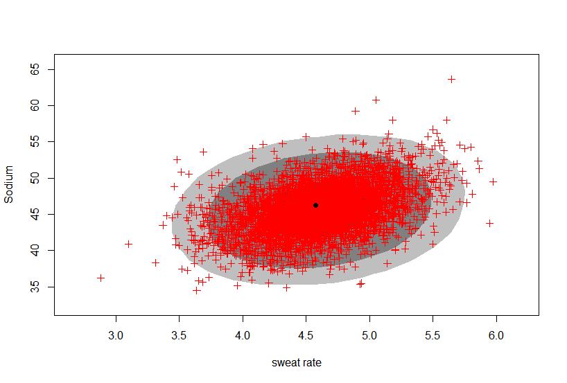
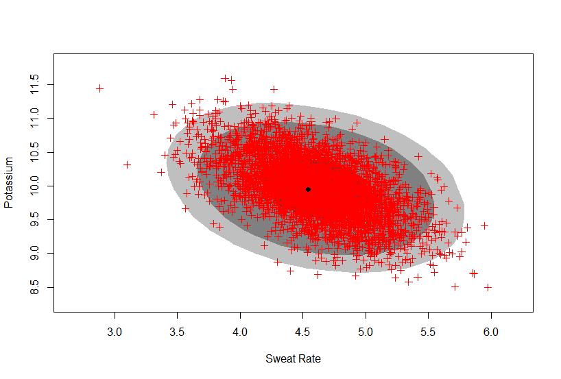
12 hdr1 <- hdr.2d(x,y) plot(hdr1, pointcol="red", show.points=true, pch=3, xlab="sweat rate", ylab="sodium") hdr2 <- hdr.2d(x,z) plot(hdr2, pointcol="red", show.points=true, pch=3, xlab="sweat Rate", ylab="potassium") hdr3 <- hdr.2d(y,z) plot(hdr3, pointcol="red", show.points=true, pch=3, xlab="sodium", ylab="potassium") For the sweat, we get our results from the simulation to be Sweat has the quantiles 2.5% 50% 97.5% And a mean of We have 95% probability that Sweat rate is between and

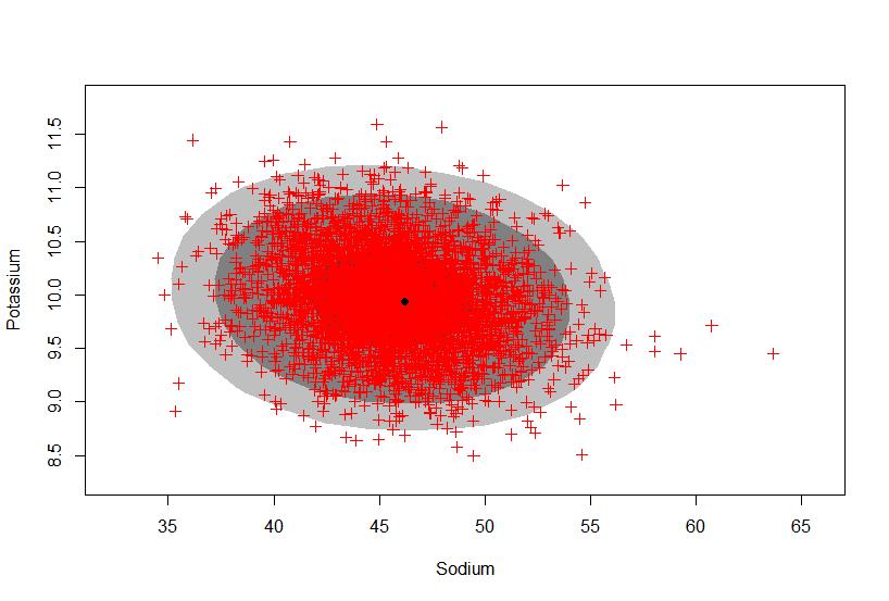
13 For our Sodium data, we get our results from our simulation to be Sodium has the quantiles 2.5% 50% 97.5% and a mean of We have 95% probability that Sodium levels are between and

14 The results from our simulation for potassium yield Potassium has the quantiles 2.5% 50% 97.5% and a mean of We have 95% probability that potassium levels are between and Looking at the pairwise relationship, we get the graphs

Bayesian GLMs and Metropolis-Hastings Algorithm

Bayesian GLMs and Metropolis-Hastings Algorithm We have seen that with conjugate or semi-conjugate prior distributions the Gibbs sampler can be used to sample from the posterior distribution. In situations,