Multigrid Solution of the Debye-Hückel Equation

Transcription

1 Rochester Institute of Technology RIT Scholar Works Theses Thesis/Dissertation Collections Multigrid Solution of the Debye-Hückel Equation Benjamin Quanah Parker Follow this and additional works at: Recommended Citation Parker, Benjamin Quanah, "Multigrid Solution of the Debye-Hückel Equation" (2013). Thesis. Rochester Institute of Technology. Accessed from This Thesis is brought to you for free and open access by the Thesis/Dissertation Collections at RIT Scholar Works. It has been accepted for inclusion in Theses by an authorized administrator of RIT Scholar Works. For more information, please contact

2 Multigrid Solution of the Debye-Hückel Equation by Benjamin Quanah Parker A Thesis Submitted in Partial Fulfillment of the Requirements for the Degree of Master of Science School of Mathematical Sciences College of Science Thesis Committee: David S. Ross Chris W. Wahle George M. Thurston Rochester Institute of Technology Rochester, NY May 17, 2013

3 Abstract Multigrid algorithms are fast solvers for elliptic partial differential equations. In this thesis, we apply multigrid methods to the model of protein charge-regulation of Hollenbeck, et al. The model of protein charge-regulation requires computing work of charging matrices for two low dielectric spheres in a salt solution, which in turn requires many solutions of the linearized Poisson-Boltzmann equation, or the Debye-Hückel equation. We use multigrid methods to reduce the run time of computing solutions to the Debye-Hückel equation, and compare the results of some simple and more complicated examples. Using the work of Brandt and others, we also construct an interpolation scheme that takes the potentially complicated behavior of the coefficient into account.

4 Introduction Introduction to Multigrid Multigrid methods are a set of algorithms used to solve boundary value problems which have had notable success in creating fast and accurate numerical solutions for elliptic partial differential equations. Multigrid methods are comprised of different working pieces, or components. These components consist of prolongation, or interpolation to finer grids, restriction of numerical approximations to coarser grids, and smoothing of errors. The creation and success of multigrid methods stems from research conducted by Brandt, Hackbush, and others [8]. Multgrid Methods are ideal for solving linear, elliptic partial differential equations. These methods have also been extended to other classes of problems, including hyperbolic and parabolic partial differential equations [36]. When solving linear elliptic partial differential equations, one obtains greater accuracy by solving the given problem on a large set of points. Brandt notes that as the problem becomes larger in size, the resources used are often wasted because the size of the discrete problem has a notable influence on the accuracy of the numerical solution [8]. Multigrid methods are a means of taking these large problems and solving related, smaller problems which provide precise numerical solutions at a reduced cost. That is, one solves smaller problems on coarser grids that will provide approximations to the same problems on finer grids; these methods save time and memory resources while providing precise numerical solutions to partial difi

5 ferential equations. The basic components of multigrid methods are that of smoothing, restriction, and interpolation. As Brandt [8] notes, the error can be represented as a Fourier Series, on which the smoother acts to dampen highly-oscillatory, or high frequency errors; one can employ the Jacobi or Gauss-Seidel method to use as a smoother. Since the convergence of these methods as stand-alone solvers depends on the size of the problem, convergence begins to slow down once there are no more high-frequency errors to dampen. The remaining errors are of low-frequency, and for the given size of problem, do not oscillate rapidly relative to the scale of the grid: At this point, one switches to a coarser problem and solves a related problem for the error, ii

6 or correction. This approximation of the correction is then interpolated to the fine grid. Coarse Error Approximation Interpolation to Fine Error Z Z x x y y The interpolated correction is added to the approximation on the fine grid. One then performs additional sweeps of the smoother to the new approximation on the fine grid. Adding Fine Error to Swept Guess Post Sweeps of New Approximation Z Z x x y y The same components of multigrid are then applied to the error, at which point the error is added back to the original numerical approximation and smoothing is applied again. One typically applies this process repeatedly until the desired accuracy is obtained. Variants of this process include the V-Cycle, W-Cycle, and the Full-Multigrid Cycle which we introduce in Chapter 3. iii

7 The Debye-Hückel Equation For this thesis, we are interested in finding fast numerical solutions to the Debye-Hückel equation below given by Hollenbeck et al. [13]: (ɛ ϕ) + κ 2 ϕ = ρ. This equation is a linearized Poisson-Boltzmann equation. The linearization corresponds to the Debye-Hückel Theory of dilute electrolyte solutions [22]. In the above equation, ɛ is the dielectric coefficient, κ is the Debye screening parameter, and ρ is the charge distribution. The functions ɛ, the dielectric coefficient, is a measure of the amount of charge which a medium, otherwise known as a dielectric, can store charge. Similarly, κ 2 represents the ionic strength of the salt solution in which the proteins are immersed, and varies in space depending upon the composition of the solution the proteins inhabit (citation here!). The work-of-charging matrices [13] to be computed for the model of protein charge regulation requires many solutions of the Debye-Hückel equation because of the numerous configurations of charged sites on the proteins. Developing a fast solver for this equation is therefore important to further progress in research. For the model developed by Hollenbeck, et al. [13], the proteins are represented by two low-dielectric spheres immersed in a salt solution. The phenomenon of charge regulation influences the attraction between protein molecules [13]. Professor Thurston and his co-workers at RIT are particularly interested in its influence on the alpha-, beta-, and gamma-crystallin proteins in the lens of the human eye, and its role in cataract disease. The charged state of a protein varies with time in an ionic solution, as random thermal agitation and electrical attraction combine to attract protons to chargeable sites on the protein and to dislodge them. The statistics of this random process are studied iv

8 through work-of-charging matrices, matrices that represent the influences of chargeable sites on one another via electrical potentials. To compute such work-of-charging matrices one must solve a Debye-Huckel equation for each chargeable site on the protein configuration of interest. The RIT group is studying configurations with chargeable sites, so the computation of a single work-of-charging matrix requires the solution of that number of three-dimensional Debye-Huckel problems. Speeding up these calculations is important to the progress of this research. In the problems in which the RIT group is interested, the proteins are represented as lowdielectric spheres in a high-dielectric ionic solution. In this model of protein charge-regulation, both the dielectric coefficient ε and the Debye screening parameter κ are discontinuous, piecewise constant functions of position. We will construct and tailor the standard multigrid method components to accurately represent the numerical solutions of the electric potential ϕ. v

9 Literature Review of Multigrid: Prior and Current Research The multigrid methods gained widespread attention, in part from an early paper by Brandt [8]. This family of methods combines corrections of numerical solutions to boundary value problems with smoothing methods such as Gauss-Seidel to obtain fast and precise numerical methods for solving elliptic partial differential equations. Brandt introduces a number of multigrid algorithms used to solve linear and non-linear elliptic partial differential equations. In addition, Brandt explains how one can derive smoothing and convergence factors that give estimates for the efficiency and speed of these methods [8]. One may use other methods such as iterant recombination to improve the accuracy of numerical solutions obtained using multigrid. [36]. Another approach involves the use of Krylov Subspace methods such as the Conjugate Gradient method. Pflaum, for example, introduces the use of the Conjugate Gradient method into multigrid methods. Pflaum s results showed that inserting a V-Cycle after every tenth iteration gave favorable errors when dealing with non-smooth and jumping coefficients [38]. Others have looked at modifiying specific components of the multigrid algorithm with notable success. The methods that have been improved focus on the prolongation and restriction operators, while others have focused on iterant recombination and residual scaling [48 50]. The latter of these methods accelerates the convergence of the multgrid methods when slow convergence is detected. As is noted by Zhang [46], smoothing the error components can also come at a certain cost, particularly since SOR may not distinguish between low- and high-frequency error components; while some may be reduced, others will not be affected depending on the parameter ω chosen for the relaxation methods. As a result, Zhang derives two relaxation parameters which reduce both low and high frequencies. vi

10 In addition to accelerating convergence, other methods have been adapted to deal with discontinuous coefficients. Zeeuw [45], for example, creates a black box multi-grid solve for linear elliptic partial differential equations, while Alcouffe, Brandt, Dendy, and Painter [2] uses finite volume type methods and a modified interpolation operator to solve elliptic partial differential equations on rectangular domains. While observing favorable results and convergence rates in each case, the results assume that the interface at which the discontinuity occurs aligns or is directly on the gridlines of the grid on which these problems are solved. Others such as Coco [11] have developed methods that deal with discontinuous coefficients where the discontinuities occur at arbitrary interfaces in the computational domain. The results of such methods are second order accurate in the infinity norm for one and two-dimensional problems, as well as convergence rates close to those of standard multigrid methods. vii

11 Chapter 1 Motivation and Objectives The motivating factors for conducting this research are the speed and precision to which linear elliptic partial differential equations can be solved using multigrid methods. Many have applied multigrid methods to different classes of problems, including the Navier-Stokes Equations [24, 51], the Steady-State Euler equations [7, 12], convection-diffusion equations [14], and anisotropic partial differential equations [35]. We focus on fine-tuning certain components of the multigrid method to increase the convergence rate of the overall algorithm. In addition, this research seeks to understand the interplay of the number of grids, grid step sizes, the relaxation schemes used, and how an optimal solver can be created when taking these factors into consideration. To explore these questions, we look to modify specific components of the multigrid algorithm which provide the greatest precision while minimizing the run time and computational work of the algorithm. Since the coefficients ε and κ may have steep gradients in certain parts of the domain, we create interpolation and restriction operators which take the behavior of the coefficients into account. We explore this concept further in the third chapter. To begin, one must first understand the interworking components of the multigrid algo- 1

12 rithms. We look at the V, W, and Full-Multigrid cycles as examples for solving linear partial differential equations. We direct our focus on devising new methods tailored to specific components of the multigrid algorithms, including prolongation (interpolation), restriction, and relaxation methods. In general, one can extend a two-grid analysis of such methods to algorithms that use multiple grids [36]. For linear elliptic partial differential equations with constant coefficients, the discretization of the partial differential equation u = f, x Ω with suitable (Dirichlet) boundary conditions is given by a matrix equation Au = f, (1) where A is a symmetric, positive-definite matrix, u is an array of unknown values of the continuous solution u in the domain Ω, and f is the array of the values of the right-hand-side function f at the corresponding grid points in the domain Ω. To solve the discretized partial differential equation, we need to define the space over which we are providing numerical solutions. We let Ω k, k = 1, 2,..., m be a heirarchy of grids which we use to solve a given partial differential equation. That is, for a domain Ω and boundary Ω, we let Ω k = {(x, y) Ω Ω : x = ih (k) x, y = jh (k) y }, 2

13 where h (k) x and h (k) y are the grid step sizes in the x- and y-directions on the kth grid, and i, j Z. The solution to the discrete problem (1) is defined on the finest grid Ω k. As previously mentioned, the methods we are using are restricted to the V, W, and Full- Multigrid Methods for the problems in which we are interested. We provide examples for the model problem, as well as problems whose coefficients vary in two and three space dimensions. We also derive a new interpolation operator in chapter 3. This scheme is compared to bilinear interpolation for use in the model problem given in chapter 3 and the linearized Poisson Boltzman Equation, otherwise known as the Debye-Hückel equation given by (ɛ φ) = κ 2 φ ρ, where ɛ is the dielectric coefficient, φ is the electric potential, κ is the Debye screening parameter, and ρ is the charge distribution [13]. We will also compare existing methods that have fine-tuned current solvers for elliptic partial differential equations, and extend them in two ways: The first involves making additions to the multigrid components that will accelerate the rate of convergence of the multigrid methods, including the V, W, and FMG cycles. We will also test the performance of this algorithm in a three-dimensional setting by using the model elliptic PDE and the Debye-Hückel equation. 3

14 Chapter 2 Multigrid Basics 2.1 Introduction The methods we will use to analyze error and convergence of the new scheme include Local Mode (Fourier) Analysis and the spectral properties of the proposed multigrid operator [8,36]. This will give insight into how the operator affects the numerical approximations and error over the course of the scheme, while the spectral radius of the operator will provide an estimate of the factor by which error is reduced after each cycle. 2.2 The Model Problem As a start to analysis, many have used the model Poisson Equation with homogeneous boundary conditions, given by u = f, x Ω u = 0, x Ω, 4

15 where we let Ω = (0, 1) 2, the unit square. For two space dimensions, this reduces to ( ) 2 u x + 2 u = f. 2 y 2 Using separation of variables on the corresponding equation u = λu, one can show that the eigenfunctions of u are given by u m,n (x, y) = sin(mπx) sin(nπy), where m and n are positive integers. To move to the discrete case, we need to solve the above partial differential equation on a grid of discrete points that coincides with the original domain. Define Ω k = {(x, y) Ω : x = ih x, y = jh y } where i, j Z. We also define the boundary of the discrete domain Ω k = {(x, y) Ω : x = ih x, y = jh y }. In practice, however, one can take Ω k to be the set of all such discrete points that lie in the interior of the original domain and on the boundary. In addition to the discrete domain Ω k, otherwise known as the fine grid, multigrid methods solve analogous problems for the error, or corrections on coarser grids. For a given fine grid, the step sizes on the next coarsest grid are doubled. The step sizes h x and h y are taken to 5

16 be 2h x and 2h y on the coarse grid, which Brandt refers to as the standard coarsening [8]. We then define the next coarsest grid as Ω k 1 := {(x, y) Ω Ω : x = 2ih x, y = 2jh y }, where again i and j are taken to be integers ranging over appropriate values. When moving to the discrete equation, we define the following operator and grid functions: Definition For the discrete problem, we define L h (L k ) as the discrete laplace operator on the kth grid with a grid step size h. Throughout this paper, we use the above two notations interchangeably. We also take f h (f k ) to be the right-hand-side grid function for the discrete problem on the kth grid, and u h (u k ) be the grid for which we seek a solution on the kth grid. For the corresponding discrete equation L h u h = f h, we obtain the similar eigenfunctions as above [36], which we show further in Chapter 4 of this thesis. In this case, the eigenfunctions are defined over the set of points Ω h = {(x, y) R 2 x = ih x, y = jh y, i, j Z}. 6

17 The use of local Fourier analysis will show how these eigenfunctions are affected by the Coarse Grid Correction method and the use of various smoothers. It is known, for example, that the eigenfunctions of the Jacobi smoothers are the same as those for the Laplace operator, making the analysis simple even though the Jacobi method has a larger smoothing factor than Gauss-Seidel and SOR [36]. One can perform similar analysis for Gauss-Seidel and SOR smoothers, though they do not share the same properties with the discrete operator that the Jacobi smoother does [18]. 2.3 Prolongation and Restriction The prolongation (interpolation) operator, often denoted I k+1 k or I2h h, transfers a grid function u k 1 (u 2h ) defined on a coarse grid Ω k 1 to the next finest grid Ω k. In two dimensions, we can interpolate a given function to the next grid by bilinear interpolation [36]: u 2h (x, y) if (x, y) Ω 2h 1 (u 2 2h(x h, y) + u 2h (x + h, y)) if (x, y) Ω 2h \ X 2h u h (x, y) = 1 (u 2 2h(x, y h) + u 2h (x, y + h)) if (x, y) Ω 2h \ Y 2h 1 (u 4 2h(x h, y h) + u 2h (x h, y + h)+ u 2h (x + h, y h) + u 2h (x + h, y + h)) if (x, y) Ω h \ Ω 2h Here, we denote the set of coarse x and y points as X 2h and Y 2h, respectively. For the restriction operator, we give three rules below. Assume that (x, y) is a point in Ω h Ω 2h : 7

18 u 2h (x, y) = u h (x, y) (1) u 2h (x, y) = 1 8 (4u h(x, y) + u h (x h, y)+ u h (x + h, y) + u h (x, y h) + u h (x, y + h)) (2) u 2h (x, y) = 1 16 (4u h(x, y)+ 2u h (x h, y) + 2u h (x + h, y) + 2u h (x, y h) + 2u h (x, y + h) u h (x h, y h) + u h (x h, y + h) + u h (x + h, y h) + u h (x + h, y + h)) (3) Rules (1), (2), and (3) are called injection, half-weighting, and full-weighting, respectively [36]. For full-weighting, one can show that this restriction operator is the transpose of the interpolation operator up to a constant, i.e. I h 2h = c(i 2h h ), c 0. This comes from the definition of the stencils for full-weighting and interpolation. On a given grid Ω k 1, the stencil for interpolating a given point to the fine grid is given by (3.3.3) while for full-weighting restriction we have 8

19 (3.3.4) We can interpret the two stencils as follows: The center value in the first stencil corresponds to the new fine value we are initializing on the fine grid, as are the corresponding values on the same row and column as the center value. Distributing the factor of 1/4 inside of the stencil gives 1/4 1/2 1/4 1/2 1 1/2 1/4 1/2 1/4 Thus, for the center value we set it as the arithmetic average of the surrounding coarse points at the corners. The other values with the weight 1/2 correspond to taking the fine value to be the average of the two adjacent coarse points at the corners of the stencil. For the full-weighting stencil, the values inside the stencil correspond to the weights assigned to the surrounding fine points. The point in the center of the stencil is the fine point that corresponds to the coarse point whose value we are setting. As an example in two dimensions, suppose we are solving a problem with zero Dirichlet boundary conditions on the unit square Ω = (0, 1) 2. We order the points in the domain in a lexicographical order, so that the interior grid points at which we find our solution are ordered from smaller to larger x- and y-values. For this example, we assume that the coarse grid Ω k 1 contains nine points in the interior of the domain. 9

20 1/ / /4 1/ / /4 1/ / / / /2 1/ /2 1/ / / / / / /4 1/4 0 1/4 1/ Ik 1 k 0 1/ / = 0 1/4 1/4 0 1/4 1/ / / / / / /2 1/ /2 1/ / / / /4 1/ / /4 1/ / /4 For the restriction operator I k 1 k, we take the transpose of the above matrix and multiply by a factor of 1/4, which corresponds to the stencil given in (3.3.4). Similar stencils and matrices can be derived for the corresponding problem in three space dimensions. 10

21 2.4 Operator-Based Interpolation For smooth, continuous coefficients, bilinear interpolation is the favored choice in multigrid methods. For problems such as the Debye-Hückel equation (ɛ ϕ) + κ 2 ϕ = ρ presented by Hollenbeck et al. [13], one must exercise more caution in tailoring multigrid methods to handle potentially steep gradients in the coefficients ɛ and κ. Further challenges may arise when the coefficients (in particular, ɛ) are discontinuous. To amend this problem, we shall use the results of (cite Brandt source that uses the volume differencing scheme) and [36] to create an interpolation operator which is second order and satisfies the jump conditions of an elliptic partial differential equation with a jump condition at an interface in the interior of the domain. We begin by looking at interpolating the course grid approximation to the next finest grid. It should be noted that although [2] uses a volume-type discretization, we can still obtain a feasible interpolation scheme using a similar approach with finite differences. For the value of the numerical solution on the fine grid, we seek to satisfy the following condition given in [36]: L h I h 2hϕ 2h = 0. That is, we assume that the function satisfying the original partial differential equation is approximately linearly on a small portion of the domain. Not that in the case of a constant coefficient ɛ, the above formulations yield bilinear interpolation. In three and higher dimen- 11

22 sions, the approach we take below is similar. For now, let ϕ h := I h 2h ϕ 2h. We begin by creating an interpolation scheme for the fine grid value ϕ ij that lies on a coarse y-line and fine x-line. Thus, the above condition on the interpolation scheme reduces to interpolation in the x-direction while y is held constant: L h I h 2hϕ 2h = 0 = ɛ i+1/2,j ϕ i+1,j + (ɛ i+1/2,j + ɛ i 1/2,j )ϕ ij ɛ i 1/2,j ϕ i 1,j h 2 = 0 = ϕ ij = ɛ i 1/2,jϕ i 1,j + ɛ i+1/2,j ϕ i+1,j ɛ i 1/2,j + ɛ i+1/2,j We can derive a similar approximation for the value of ϕ ij which lies on a fine y-line and coarse x-line. As before, this reduces to a discrete analogue of the derivative with respect to just y because we are treating x as constant. L h I h 2hϕ 2h = 0 = ɛ i,j+1/2 ϕ i,j+1 + (ɛ i,j+1/2 + ɛ i 1/2,j 1/2 )ϕ ij ɛ i,j 1/2 ϕ i,j 1 h 2 = 0 = ϕ ij = ɛ i,j 1/2ϕ i,j 1 + ɛ i,j+1/2 ϕ i,j+1 ɛ i,j 1/2 + ɛ i,j+1/2 Finally, we find an approximation to the value of ϕ ij which does not lie on the coarse grid. That is, the point (x i, y j ) does not lie on an x- or y-gridline from the coarse grid. We then have L h ϕ h = ( ) ɛi+1/2,j ϕ i+1,j (ɛ i+1/2,j + ɛ i 1/2,j )ϕ ij + ɛ i 1/2,j ϕ i 1,j h 2 12

23 ( ) ɛi,j+1/2 ϕ i,j+1 (ɛ i,j+1/2 + ɛ i,j 1/2 )ϕ ij + ɛ i,j 1/2 ϕ i,j 1 + κ 2 ijϕ ij = 0. h 2 We then multiply the above equation through by h 2 and collect the terms with ϕ ij on one side to obtain (ɛ i 1/2,j + ɛ i+1/2,j + ɛ i,j 1/2 + ɛ i,j+1/2 + (hκ ij ) 2 )ϕ ij = ɛ i 1/2,j ϕ i 1,j + ɛ i+1/2,j ϕ i+1,j + ɛ i,j 1/2 ϕ i,j 1 + ɛ i,j+1/2 ϕ i,j+1, so ϕ ij = ɛ i 1/2,jϕ i 1,j + ɛ i+1/2,j ϕ i+1,j + ɛ i,j 1/2 ϕ i,j 1 + ɛ i,j+1/2 ϕ i,j+1 ɛ i 1/2,j + ɛ i+1/2,j + ɛ i,j 1/2 + ɛ i,j+1/2 + (hκ ij ) 2. In the above formula, note that the values ϕ i 1,j, ϕ i+1,j, ϕ i,j 1, and ϕ i,j+1 are fine-grid values obtained from the interpolation on coarse lines given above. 2.5 Work Units Another aspect of the multigrid convergence analysis comes from Brandt s use of the multigrid work unit W U, which he defines as the total work done on the finest grid over the coarse of one relaxation sweep [8]. Work units can be measured as the number of floating point operations on a given grid; if the finest grid has N points, and there are w floating point operations per grid point, then one work unit is approximately w N floating point operations. Additionally, one may also take into consideration the work it takes to interpolate and restrict numerical solutions to finer and coarser grids. Brandt notes that a majority of the computational work takes place with relaxation sweeps; the work invested in restriction and prolongation is considered negligible since it comprises around twenty percent of the 13

24 total work. Restriction and prolongation, however, are important in other regards since they affect the representation of the error frequencies on the grids. To give an estimate of the total computational work of restriction and interpolation relative to the total work in a multigrid V-Cycle (see next section), we suppose that the number of points in the x- and y-directions is N, so we seek a solution on a grid of N 2 points. We then look at multigrid in terms of four components: One application of the smoother before moving to a coarse grid and one application after returning to a fine grid, computing the residual, restriction, and interpolation. For the smoother, we employ a Gauss-Seidel smoother for the standard five-point laplacian given by u ij = h2 f ij + u i 1,j + u i+1,j + u i,j 1 + u i,j+1. 4 On any given grid, we perform five additions per grid point when computing a new value of the approximation to u(x, y). Then one work unit (WU) is approximately 5N 2 additions. Since the smoother is applied once before moving to a coarse grid and once after interpolating to a fine grid, an estimate on the total number of additions over one multigrid V-cycle is 2 (5N 2 + 5N N N ) 2 = k 1 ( 10N ) k 1 10N = 40N 2 3 additions. 14

25 After smoothing, we compute residual as follows: r ij = f ij + u i+1,j 2u ij + u i 1,j h 2 + u i,j+1 2u ij + u i,j 1 h 2. This incurs six additions per grid point on the given grid, yielding 6N 2 additions on the fine grid. Since we compute the residual on all grids but the coarsest, the estimated number of additions is given by 6N 2 + 6N N N 2 4 k 1 = 6N 2 ( k 1 6N = 8N 2 ) For restriction, we compute the values at the coarse grid points as weighted sums of the surrounding fine grid points. For each coarse grid point, the new value takes eight additions to compute. Restricting a fine grid residual to a coarse grid then takes approximately N 2 N 2 8 = 2N 2 additions. Interpolation from the coarse grid Ω k 1 to the fine kth grid takes approximately 2 N 2 N 2 + 2N 2 N 2 + 4N 2 N 2 = 2N 2 15

26 additions. Now considering the work done over all grids, and assuming we can neglect the work done on the coarsest grid, an upper bound of the total work performed by interpolation is 2N 2 + 2N N N 2 4 k 1 = 2N 2 ( k 1 2N = 8N 2 3 ) additions. We obtain a similar estimate for restriction, since on the next coarsest grid, we do about one quarter of the work we did on the previous fine grid in two dimensions. Thus, the estimated number of additions for restriction over all grids is ( 2N ) N k 1 3. Thus, the approximate percentage of work spent on interpolation and restriction combined is = = 1 5 or twenty percent. Now consider the following: Define the ratio of step sizes ˆρ = h k h k 1 between two successive grids. If we have problem in d dimensions and a mesh size ratio of ˆρ = 1, then the work 2 16

27 done on the grid G M j is given by ˆρ dj work units [8]. From this analysis, we can derive the multigrid convergence factor ˆµ, the rate by which all errors are reduced per one work unit of relaxation, assuming we ignore the computational work of restriction and interpolation [8]. Suppose that during the course of the scheme, we perform s relaxation sweeps on each level. Recall that the relaxation factor is given by µ, so that after s sweeps, the high-frequency errors have been reduced by a factor of µ s. We can then provide an upper bound of the total computational work (excluding restriction and prolongation) over each grid, given by s + sˆρ d + sˆρ 2d sˆρ (M 1)d < s 1 ˆρ d, for which we then define the multigrid convergence factor as [8] ˆµ = µ 1 ˆρd. This convergence factor represents the rate of error reduction per unit of work. 2.6 The Coarse Grid Correction Scheme One can derive multigrid methods based on the coarse grid correction scheme [36], which we give below. The two-grid correction and relaxation cycle forms the basis for methods which recurse on multiple grids, including the V-Cycle, W-Cycle, and Full-Multigrid-Cycle. For non-linear problems, one may use the Full-Approximation-Storage Method outlined by Brandt [8]. 17

28 Algorithm 1 Coarse Grid Correction (1) Provide an initial guess u 0 h on the finest grid Ω h (2) Relax u 0 h v 1 times on the grid Ω h (3) Compute the residual r h = f h L h u h (4) Restrict the residual to the next coarsest grid: r 2h = Ih 2hr h (5) Solve the error equation A 2h e 2h = r 2h (6) Interpolate the error to the next finest grid: e h = I2h h e h (7) Add the error to the initial swept-over guess: u 0 h = u0 h + e h (8) Perform v 2 additional relaxation sweeps on u 0 h 2.7 The Multilevel Operator: Definition and Derivation For the definition of the multigrid (multilevel) operator, we use the following theorem from [36]. In the theorem below, the operator I k is the identity operator on the kth grid. Theorem 1. The multigrid iteration operator M l is given by the following recursion: M 0 = 0, M k = S v 2 k (I k Ik 1 k (I k 1 M γ k 1 )(L k 1) 1 I k 1 k L k )S v 1, (k = 1,..., l). k Proof. By definition, M 0 u 0 k = 0, and for k = 1, we obtain the two-level operator M 1 = S v 2 1 (I 1 I 1 0(L 0 ) 1 I 0 1L 1 )S v 1 1 = S v 2 1 (I 1 I 1 0(I 0 M γ 0 )(L 0 ) 1 I 0 1L 1 )S v 1 1. Now assume the recursive definition holds for k 1. To show this holds true for the next level k + 1, suppose we wish to solve the fine-grid problem on the grid Ω k+1 : L k+1 u k+1 = f k+1. 18

29 We step through the multigrid process by applying the smoother on grid k + 1 v 1 times, and compute the residual on the fine grid: r k+1 = f k+1 L k+1 S v 1 k+1 u0 k+1. We then restrict this residual to the coarser grid by setting r k = I k k+1 r k+1, and approximately solve the corresponding equation L k e k = r k (1) for the correction e k. To do so, we devise an iterative scheme using the multilevel operator M k. From (1), we have that e k = L 1 k r k. The correction e k also satisfies (I k M k )e k = (I k M k )L 1 k r k (2) since M k is nonsingular and a convergent operator, i.e. M k < 1. In addition, we also assume M k has no zero eigenvalues. Then (2) can be written as e k = M k e k + (I k M k )L 1 k r k (3), 19

30 and so we define the following (multilevel) iterative scheme: e n+1 k = M k e n k + (I k M k )L 1 k r k (4). Applying this iteration γ times to the iterate e 0 k with e0 k = 0 yields e γ k = (I k M γ k )L 1 k r k. Once this approximation to the correction has been given on the coarse grid, we interpolate this correction to the fine grid and add it to the approximation of the numerical solution, and perform v 2 addition smoothing sweeps: S v 2 k+1 (Sv 1 k+1 u0 k+1 + I k+1 k e γ k ). Placing these steps together yields S v 2 k+1 (Sv 1 k+1 u0 k+1 + I k+1 k (I k M γ k )L 1 k Ik k+1(f k+1 L k+1 S v 1 k+1 u0 k+1)). Simplifying the above expression yields k+1 (I k+1 I k+1 k (I k M γ k )L 1 k Ik k+1l k+1 )S v 1 k+1 u0 k+1+ S v 2 S v 2 k+1 Ik+1 k (I k M γ k )L 1 k Ik k+1f k+1, with 20

31 M k+1 = S v 2 k+1 (I k+1 I k+1 k (I k M γ k )L 1 k Ik k+1l k+1 )S v 1 k Common Multigrid Algorithms Introduction The following sections present common algorithms used in multigrid methods. Further details of these algorithms may be found in [36] V-Cycle The following is the algorithm for the V-Cycle: Algorithm 2 V-Cycle (1) Relax u 0 k v 1 times on the grid Ω h (2) Compute the residual r k = f k L k u k (3) If k > 1, call VCYCLE(A k 1, v k 1, r k 1 ) with v k 1 = 0 as an initial guess (4) Else if k = 1, solve A k v k = r k directly (5) Interpolate the error to the next finest grid: ṽ k = I k k 1 v k (6) Add the error to the initial swept-over guess: u 0 k = u0 k + ṽ k (7) Perform v 2 additional relaxation sweeps on u 0 k (8) Return the new approximation u 0 k W-Cycle The following is the algorithm for the V-Cycle: 21

32 Algorithm 3 W-Cycle (1) Relax u 0 k v 1 times on the grid Ω h (2) Compute the residual r k = f k L k u k (3) For n = 1, 2 (4) If k > 1, call WCYCLE(A k 1, v k 1, r k 1 ) with v k 1 = 0 as an initial guess (5) Else if k = 1, solve A k v k = r k directly (6) Interpolate the error to the next finest grid: ṽ k = I k k 1 v k (7) Add the error to the initial swept-over guess: u 0 k = u0 k + ṽ k (8) Perform v 2 additional relaxation sweeps on u 0 k (9) End for (10) Return the new approximation u 0 k FMG-Cycle The following is the algorithm for the Full Multigrid (FMG) Cycle. Here, r denotes the number of applications of the V-Cycle on a given grid. Other cycles may also be used in place of the V-Cycle [36]. Algorithm 4 FMG-Cycle (1) Solve L 1 u 1 = f 1 exactly on the coarsest grid to obtain u F 1 MG (2) Interpolate this guess using FMG-Interpolation to the next grid Ω 2 (3) For k = 2,..., M (4) Call V CY CLE r (A k, u k, f k ) (5) If k < M (6) Use FMG Interpolation on u k to obtain a guess on the next highest grid Ω k+1 (7) End If (8) End For 2.9 Norm Estimates and Theorems We give the following error estimate theorems for the multigrid methods for the γ-cycle (γ 2) and the FMG-cycle. For γ = 1, the error estimates in the following theorem are not independent of the grid step size(s), so a more thorough treatment is needed [36]. For the following theorem, we first provide definitions of the operators given in the state- 22

33 ment. The following corollary from Trottenberg, Oosterlee, and Schüller [36]: Corollary. For k = 1,..., l 1, the equations M k+1 = M k k+1 + A k+1 k (M k ) γ A k k+1 hold, where A k+1 k := (S k+1 ) v 2 I k+1 k : G(Ω k ) G(Ω k+1 ) A k k+1 := (L k ) 1 I k k+1l k+1 (S k+1 ) v 1 : G(Ω k+1 ) G(Ω k ) and Proof. From Theorem 1, we have that M k k+1 = S v 2 k+1 (I k+1 I k+1 k (L k ) 1 I k k+1l k+1 )S v 1 k+1. M k+1 = S v 2 k+1 (I k+1 I k+1 k (I k (M k ) γ )(L k ) 1 I k k+1l k+1 )S v 1 k+1, which may be written as S v 2 k+1 (I k+1 I k+1 k I k (L k ) 1 I k k+1l k+1 + I k+1 k (M k ) γ (L k ) 1 I k k+1l k+1 )S v 1 k+1. This simplifies to S v 2 k+1 (I k+1 I k+1 k (L k ) 1 I k k+1l k+1 )S v 1 k

34 S v 2 k+1 Ik+1 k (M k ) γ (L k ) 1 I k k+1l k+1 S v 1 k+1 = S v 2 k+1 (I k+1 I k+1 k (L k ) 1 I k k+1l k+1 )S v 1 k+1 + Ak+1 k (M k ) γ A k k+1 = Mk+1 k + A k+1 k (M k ) γ A k k+1. The following theorem from [36] gives estimates for the norm of the multigrid operator for γ 2. Theorem 2. Let the following estimates hold uniformly with respect to k: M k k+1 σ, A k+1 k A k k+1 C. Then we have M l η l. where η l is recursively defined as η 1 = σ, η k+1 = σ + Cη γ k, (k = 1, 2,..., l 1). If we additionally assume that 4Cσ 1 and γ = 2, we obtain the following uniform estimate for M h = M l (h = h l ): M h η := 1 1 4Cσ 2C 2σ, l 1. Before proving the above theorem, we require the following Lemmas. 24

35 Lemma 1. Let f(η) = Cη 2 + σ and let g(η) = mη + σ with m = η σ η, η = 1 1 4Cσ, and 4Cσ 1. The sequences {η 2C k } k=1 and {µ k} k=1 with η k+1 = f(η k ) = Cη 2 k + σ, µ k+1 = g(µ k ) = mµ k + σ, and η 1 = µ 1 = σ are monotonic and bounded. Hence, both sequences converge [40]. Proof. To complete the proof, we first show that µ k is monotonic and bounded for all positive integers k. The fact that η k is bounded follows from a further proof that η k µ k for all integers k 1. We prove µ k is bounded by induction on k. Indeed, µ 1 < µ 2 since σ < σ + mσ. Now suppose this holds for some integer k 2. By the inductive step we have µ k 1 < µ k. Since g is strictly increasing, it follows that g(µ k 1 ) < g(µ k ) which implies µ k < µ k+1. To show that {µ k } k=1 is bounded, observe that the linear recurrence relation formed by 25

36 the sequence {µ k } k=1 has a closed form solution when we trace down to the base case of µ 1 = σ : µ k = mµ k 1 + σ = m 2 µ k 2 + mσ + σ =... = m k 1 σ + m k 2 σ mσ + σ = σ 1 mk 1 m = σ 1 mk 1 η σ η = σ 1 mk σ η = η (1 m k ). This expression approaches η from below as k. Now we show that {η k } k=1 is monotonic by induction on k. Observe that η 1 < η 2 since σ < σ +C(σ ) 2. Now assume that η k 1 < η k holds for some integer k 2. Since f is also strictly increasing on [σ, η ], we have that f(η k 1 ) < f(η k ) = η k < η k+1. Finally, we prove the claim that η k µ k for all integers k 1. As a base case, we have that η 1 µ 1 by construction, so assume that this holds for some integer k 1. The induction step gives η k µ k, so to prove the claim we use the fact that g f for all η [σ, η ]: η k+1 = f(η k ) f(µ k ) g(µ k ) = µ k+1. Thus, {η k } k=1 and {µ k} k=1 converge. The next lemma gives a proof of convergence of the sequence {η k } k=1 in the case that 4Cσ < 1. Lemma 2. Let σ = p 4C, with 0 < p < 1. Then the sequence {η k} k=1 converges to η. 26

37 Proof. It suffices to show that η η k 0 (2.1) as k. Since η is a fixed point of the map f(η) = Cη 2 + σ, (2.1) can be written as C(η ) 2 + σ Cη 2 k σ = C (η ) 2 η 2 k = C η + η k η η k = C η + η k C(η ) 2 C(η k 1 ) 2 = C 2 η + η k η + η k 1 η η k 1 =... = C k η + η k η + η k 1... η + η 2 η + η 1 η η 1 = C k ( Π k j=1 η + η j ) (η σ ). From Lemma 1, we have η j µ k and µ k η as k, so η η k+1 C k ( Π k j=1 η + η ) (η σ ) = C (Π k k 1 ) ( ) 1 4Cσ 1 1 4C p k j=1 (η σ ) = C k 4C (η σ ) = C C k (1 1 p) k (η σ ), which approaches zero as k. The next lemma gives a short proof for the convergence of {η k } k=1 in the case that σ, the norm of the two-level operator M k+1 k, is equal to 1. In this case, we have to be more 4C careful since f(η) = η 2 + σ is a nonexpansive map on the interval (σ, η ) [1], i.e. 27

38 f(η) f(ξ) K η ξ η, ξ (σ, η ), where K = 1. Lemma 3. Suppose now that the norm of the two-level operator in Theorem 2 is σ = 1 4C, so now η = 1 2C. Then the sequence {η k} k=1 converges to the unique fixed point η of the map f(η) = Cη 2 + σ Proof. We begin by showing that the fixed point of the map f(η) = Cη 2 + σ is unique. Since η is a fixed point of f, it follows that η 2 = C(η ) C = C(η ) 2 η + 1 4C = 0, which admits one root given by η = 1 ± 1 4C 1 4C 2C = 1 2C, so η is necessarily unique. To complete the proof, we utilize Theorem 2.1 from Ahmed [1]. In order to prove that the sequence {η k } k=1 converges, we must show that lim η k+1 η k = 0 (1) k and 28

39 lim η k (2) k exists. The second condition follows from Lemma 1, since it was shown that {η k } k=1 is bounded and monotonic. Thus, the sequence is Cauchy on [σ, η ] which implies condition (1) [40], so η k η as k. We now proceed with the proof of Theorem 2. Proof. We first observe that M k+1 = Mk+1 k + A k+1 k (M k ) γ A k k+1 M k k+1 + A k+1 k A k k+1 M k γ = σ + Cη 2 k = η k+1. Now under the additional assumptions, we must show that as k, η k approaches the limit point η which satisfies η = σ + Cη 2, a quadratic in η with the root η = 1 1 4Cσ. 2C Then by Lemmas 1, 2, and 3, the sequence {f(η k )} k=1 with η 1 = σ converges to the fixed point 29

40 η = 1 1 4Cσ 2C in [0, 1 2C ]. By rationalizing the denominator of η, we obtain the estimate from the above theorem: 1 1 4Cσ 2C = 1 (1 4Cσ ) 2C( Cσ ) = 2σ Cσ 2σ. The following theoretical estimates from [36] for Full Multigrid are also given: Theorem 3. Let the following assumptions hold: (1) Let the norm of the multigrid iteration operator M h be uniformly bounded: M h η < 1 (2) Let the norm of the FMG interpolation operator Π k k 1 be uniformly bounded: Π k k 1 P < 1 (3) The discretization error and the FMG interpolation error are assumed to be of order κ and order κ F MG, respectively: u u h Kh κ, (h = h k ; k = 1, 2,...), u Π k k 1u Kh κ F MG, (h = h k ; k = 1, 2,...), 30

41 In addition, assume that η r < 1 2 κ P. Then the following estimate holds for any l 1: u l u F MG l δh κ l, where δ = η r B 1 η r A, with A = 2 κ P and any bound B such that K(1 + A) + Kh κ F MG κ B. Proof. By the definition of the Full-Mulitgrid Method, we have for all l 1 u F MG l u l = (M l ) r (u l 0 u l ), with u l 0 = Π l l 1u F MG l 1. We first make use of the following identity: u 0 l u l = Π l l 1(u F MG l 1 u l 1 ) + Π l l 1(u l 1 u) + (Π l l 1u u) + (u u l ). 31

42 Then we have that u F MG l u l = (M l ) r (u 0 l u l ) η r u 0 l u l η r (P u F MG l 1 u l 1 + P u l 1 u + Π l l 1u u + u u l ) = η r (P u F MG l 1 u l 1 + P Kh κ l + Kh κ F MG l + Kh κ l ). Let δ l = u F MG l above estimate is written as u l /h κ l, l 1. After dividing the above inequality through by hκ l, the δ l η r (Aδ l 1 + AK + Kh κ F MG κ l + K), where A = 2 κ P. Now let B be any bound such that K(1 + A) + Kh κ F MG κ B, and let p = η r A. Then the above inequality may be written as δ l pδ l 1 + B where B = η r B. Expanding δ l 1 and using the fact that δ 0 = uf MG 0 u 0 h κ 0 = 0 h κ 0 = 0, we obtain δ l p l δ 0 + (1 + p + p p l 1 ) B = (1 + p + p p l 1 ) B. 32

43 This implies that δ l B 1 p = ηr B 1 η r A and so u l u F MG l δh κ l. 33

44 Chapter 3 Local Mode Analysis 3.1 Introduction and Definitions Local Mode Analysis [8] allows one to conclude the properties of multigrid, providing information about the rate at which the error is reduced and how fast the multigrid algorithm itself will converge. We begin by identifying important concepts needed before proceeding with a case analysis of the model Poisson equation. We provide definitions for the twodimensional case that can extend to any n-dimensional setting. Definition Let θ = (θ 1, θ 2 ) and x = (x 1, x 2 ) be vectors in R 2, and let G h = {(x, y) R 2 : x = ih x, y = jh y, i, j Z} be the grid with step sizes h x and h y. Then the grid function associated with the discrete operator L h is given by ϕ(θ, x) = e iθ x. One can show that the above grid functions ϕ(θ, x) are in fact the eigenfunctions of L h. Definition Let θ = (θ 1, θ 2 ) be a vector in R 2. Define θ to be a low-frequency 34

45 component if θ [ π 2, π 2 ] 2, where θ := max{ θ 1, θ 2 }. Otherwise, define θ to be a high frequency component if θ [ π, π] 2 \ [ π 2, π 2 ] 2. Consequently, define the following sets T high and T low [36] as T high = { [ θ R 2 : θ π 2, π ] } 2 2 and T low = { [ θ R 2 : θ [ π, π] 2 \ π 2, π ] } 2. 2 These sets represent the high- and low-frequency components, respectively. 3.2 H-Ellipticity of the Discrete Laplace Operator To formulate a discrete solution to the original problem, we need to assess how well the discrete operator satisfies the properties of the original elliptic operator L =. We arrive at the following definition from Brandt [36]: 35

46 Definition Let L h be the discrete anologue of the differential operator L. The h-ellipticity measure of the operator L h is defined as E h (L h ) = min { L h (θ) : θ T high } max { L h (θ) : π θ π}, with 0 < c E h (L h ) 1. One can show that the 5-point Laplace operator given by L h (u) = u i+1,j 2u ij + u i 1,j h 2 u i,j+1 2u ij + u i,j 1 h 2 has a nonzero h-ellipticity. We observe this is the case by applying the operator to the mode e iθ x : L h e iθ x = 1 h 2 ( 4e iθ x e iθ 1 e iθ x e iθ 1 e iθ x e iθ 2 e iθ x e iθ 2 e iθ x) = L h e iθ x = L h (θ)e iθ x, where L h (θ) = 1 h 2 ( 4 e iθ 1 e iθ 1 e iθ 2 e iθ 2 ). Then we have that E h (L h ) = 0.25, which occurs when θ = (0, π 2 ) [36]. 36

47 3.3 Local Mode Analysis The tools that we will employ for error analysis are those upon which multigrid is based: Local Fourier Analysis and the operator properties of the multigrid methods, expressed as operator equations [8]. The Local Fourier analysis allows one to show what happens to certain frequencies and components of the error, and the effects of the method can be seen by how the method itself acts on the eigenfunctions (derived in section 3.1) of the discrete differential operator. Local Fourier analysis serves as a useful framework from which one can view the effects of smoothing operators and the entire multigrid scheme on the low- and high-frequency components of the error [8, 18, 36]. Suppose we are attempting to solve a linear elliptic partial differential equation given by a 2 u x 2 + c 2 u y 2 = f with some prescribed boundary conditions, and where a and c are constant coefficients. Furthermore, suppose we are discretizing by finite differences using a second order approximation to the second partial derivatives of u, and that our step sizes in the x- and y-directions are the same. On the kth grid, we have that the exact grid function u k satisfies. a uk m+1,n 2u k mn + u k m 1,n h 2 k + c uk m,n+1 2u k mn + u k m,n 1 h 2 k = f k mn (1) Where f k mn is the right-hand-side function on the kth grid evaluated at the point (x m, y n ) and h k is the step size on grid k. When using Gauss-Seidel, we update the values u mn, u m 1,n, and u m,n 1 of an approximate solution u with new values ū mn, ū m 1,n, and ū m,n 1 to obtain 37

48 the following: a u m+1,n 2ū mn + ū m 1,n h 2 k + c u m,n+1 2ū mn + ū m,n 1 h 2 k = f k mn (2) This new approximation ū may not immediately satisfy the first finite difference equation above, and addition applications, or sweeps, of Gauss-Seidel may be necessary to improve it. Nonetheless, we introduce an important quantity, the smoothing factor, given by µ = v v, v = uk ū, v = u k u, where v and v are the error functions before and after one application of Gauss-Seidel (or any other smoother). In order to determine the smoothing factor in practice, we let θ = (θ 1, θ 2 ) be the Fourier components of the error and write v and v as v = A θ e i(mθ 1+nθ 2 ) and v = Āθe i(mθ 1+nθ 2 ). Thus, subtracting (2) from (1) and multiplying through by h k yields a ( (u k m+1,n u m+1,n ) 2(u k mn ū mn ) (u k m 1,n ū m 1,n ) ) + c ( (u k m,n+1 u m,n+1 ) 2(u k mn ū mn ) (u k m,n 1 ū m,n 1 ) ) = 38

49 a(v m+1,n 2 v mn v m 1,n ) + c(v m,n+1 2 v mn v m,n 1 ) = 0, or in terms of theor Fourier representations, a ( A θ e i((m+1)θ 1+nθ 2 ) 2Āθe i(mθ 1+nθ 2 ) + Āθe i((m 1)θ 1+nθ 2 ) ) + c ( A θ e i(mθ 1+(n+1)θ 2 ) 2Āθe i(mθ 1+nθ 2 ) + Āθe i(mθ 1+(n 1)θ 2 ) ) = 0. By dividing through by the common factor e i(mθ 1+nθ 2 ) and collecting like terms with A θ and Ā θ, we obtain a ( A θ e iθ 1 2Āθ + Āθe iθ 1 ) + c ( A θ e iθ 2 2Āθ + Āθe iθ 2 ) = 0 or A θ (ae iθ 1 + ce iθ 2 ) + Āθ(ae iθ 1 + ce iθ 2 2a 2c) = 0. Thus, the convergence factor µ can be expressed as µ(θ) = Āθ A θ = ae iθ1 + ce iθ2 2a + 2c ae iθ 1 ce iθ 2. Since we seek to find the worst factor by which error is reduced for high-frequency components, we seek to find the θ which maximizes µ subject to the constraint that ˆρπ θ π, 39

50 where θ = max{ θ 1, θ 2 } and ˆρ is the ratio of the current and next coarsest grid steps, i.e. ˆρ = h k h k 1. This allows one to find the worst factor µ by which high frequency error components are reduced at each step. For a Poisson equation with a = c, we have µ = [8]. The smoothers perform well initially, but convergence slows down after the first two or three sweeps. This corresponds to a smoothing of the low-frequency errors, but the purpose of multigrid is not to eliminate the low-frequency error components on the given grid. When we move to coarser grids, the lower frequency components become high frequencies on those grids. This allows those same frequencies to be reduced while even lower frequencies are approximated more precisely before we add them back to the numerical approximation of the solution. This analysis allows one to pick or create a suitable smoother that accounts for the behavior of the partial differential equation [8] Spectral Properties of the Multigrid Operators Another component of the analysis involves computing the largest eigenvalue of the multigrid operator to see at what rate the numerical approximation converges to the solution. From the section on the Coarse Grid Correction cycle, we can write the algorithm in terms of matrices and vectors as u 1 h = S v 2 (u 0 h + I h 2hL 1 2h I2h h (f h L h S v 1 u 0 h)) = S v 2 (u 0 h + M(f h L h S v 1 u 0 h)) = S v 2 (I MS v 1 L h )u 0 h + S v 2 Mf, where M = I2h h L 1 2h I2h h, I2h h from the fine grid to the coarse grid, and I h 2h is the restriction operator which transfers the approximation u0 h 40 is the interpolation operator which transfers

51 the approximation u 0 2h from the coarse grid to the fine grid. This component of the analysis looks at the spectral radius of the multigrid operator given by M 2h h = S v 2 (I MS v 1 L h ), which yields the factor by which the error is reduced at each step. Note also that the coarse grid correction scheme without smoothing yields the operator I ML h, which is known to have eigenvalues larger than 1 [36]. The use of smoothing operators, however, works in conjunction with coarse grid correction to provide the overall multigrid operator with a spectral radius that is less than 1, independent of the step size of the finest grid. 41

52 Chapter 4 Application of Multigrid to the Debye-Hückel Equation Recall that we seek to solve the Debye-Hückel. For the solutions of this equation, we use the operator-dependent interpolation described in Chapter 3. In addition to testing numerical solutions of this equation with the dielectric coefficient ε represented as a jump function at the interface of the dielectric spheres, we employ the transition function given below from [13]. e ( r R)/S ε = ε m (ε i ε m ) 1 + e ( r R)/S In this definition of ε, r is the euclidean distance from the center of the sphere, R is the radius of the sphere, and S is the characteristic length over which the change in the dielectric coefficient takes place [13]. We take S to be 0.2 Å in this case. In the following section, we use local Fourier Analysis from Chapter 4 to justify the use of the operator-dependent interpolation method. 42

53 4.1 Local Fourier Analysis of the Debye-Hückel Equation We begin by taking the same approach as in [36] by writing the differential operator L(u) = (ε u) + κ 2 u as follows: L h w + L + h w+, where L h is the portion of discrete operator stencil that acts on a previously updated approximation (or correction) w and w + is an approximation upon which an operation has yet to take place. The stencil for the Debye-Hückel equation used in two dimensions is given by ɛ i,j+1/2 L h = 1 h 2 ɛ i 1/2,j (ɛ i 1/2,j + ɛ i+1/2,j + ɛ i,j 1/2 + ɛ i,j+1/2 ) ɛ i+1/2,j + ɛ i,j 1/2 0 0 κ 2 ij 0. 0 We split this discrete operator into its constituent parts L h and L+ h as follows: 43

54 L h = 1 0 h 2 ɛ i 1/2,j (ɛ i 1/2,j + ɛ i+1/2,j + ɛ i,j 1/2 + ɛ i,j+1/2 ) 0 + κ 2 ij ɛ i,j 1/ L + h = 1 ɛ i,j+1/2 0 h ɛ i+1/2,j + κ2 ij = h 2 ɛ i,j+1/2 0 0 ɛ i+1/2,j. 0 When acting on the formal eigenfunction e iθ x, we have that [ 1 ( L eiθ x h = (ɛ h 2 i 1/2,j + ɛ i+1/2,j + ɛ i,j 1/2 + ɛ i,j+1/2 ) ) ] ɛ i 1/2,j e iθ 1 ɛ i,j 1/2 e iθ 2 + κ 2 ij e iθ x. Similarly, we have that L + h eiθ x = 1 h 2 [ɛ i+1/2,j e iθ 1 + ɛ i,j+1/2 e iθ 2 ] e iθ x. Denote by L h (θ) and L + h (θ) the formal eigenvalues computed above for L h and L+ h, respec- 44

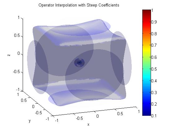
55 tively. Then the smoothing factor is given by µ(θ) = L+ h (θ) L h (θ), for which we need to find the supremum of µ over all high-frequency components θ: µ(θ) = 1 ɛ h 2 i+1/2,j e iθ 1 + ɛ i,j+1/2 e iθ 2 1 ((ɛ h 2 i 1/2,j + ɛ i+1/2,j + ɛ i,j 1/2 + ɛ i,j+1/2 ) ɛ i 1/2,j e iθ 1 ɛi,j 1/2 e iθ 2 ) + κ 2 ij = ɛ i+1/2,j e iθ 1 + ɛ i,j+1/2 e iθ 2 ɛ i 1/2,j + ɛ i+1/2,j + ɛ i,j 1/2 + ɛ i,j+1/2 ɛ i 1/2,j e iθ 1 ɛi,j 1/2 e iθ 2 + h2 κ 2 ij In the above expression ɛ i±1/2,j and ɛ i,j±1/2 is the dielectric coefficient ɛ evaluated at the half-index points (x i±1/2, y j ) and (x i, y j±1/2 ). Brandt in [8] states that one may ignore changes in the coefficient by locally treating coefficients as constant. Interfaces with strong jumps and discontinuities, however, must be taken into account because smoothing rates can deteriorate in these regions. If, for example, ɛ i+1/2,j >> ɛ i 1/2,j and ɛ i,j±1/2 are of the same order as ɛ i 1/2,j then the smoothing factor approaches 1 quickly in this region. It should be noted, however, that κ 0 can reduces the smoothing factor, especially when ɛ is smooth. For our purposes, however, the dielectric coefficient is relatively smooth when one is sufficiently far from the interface. Thus, one could use the normal differencing stencil and bilinear interpolation. Near the interface, however, we choose to use the operator-dependent interpolation defined in Chapter 3, with numerical results given in the following chapter. 45

56 Chapter 5 Numerical Results Introduction The following sections give numerical results for the application of the multigrid V-Cycle to numerous test problems and the Debye-Hückel equation. The error tables given for each problem measure the norm of the residual r = f Au after each iteration. We first give examples in two dimensions, followed by results for the Debye-Hückel equation in three dimensions D Results As en example of the utility of multigrid V-Cycle, we show the results of running the multigrid V-Cycle on the unit square Ω = [0, 1] 2 for the following problem solved by Brandt [8]: u = sin(3(x + y)), (x, y) Ω u = cos(2(x + y)), (x, y) Ω. Graphs of the solution, as well as error and residual norms, are given below. For this par- 46

57 ticular program, a total of six grids were used with an initial step size of h = 1. The table 2 below show the norms of the residuals in three norms for each run of the V-Cycle. To reduce the residual norm to 1.52E-06 in the L 2 -Norm, we had to expend approximately 26 WU. Cycle Grid Level L 1 -Norm L 2 -Norm L -Norm WU E E E+03 0E E E E E E E E E E E E E E E E-01 5E E E E E E E E E E E E E E E E E E E E E E E E E+01 47

58 Z Fortran Results: Iteration x y

59 Z Fortran Results: Iteration x y

60 Z Fortran Results: Iteration x y

61 Z Fortran Results: Iteration x y 0.2 When using six grids, running a total of ten V-Cycles took less than one second. Below we give another table or residual norms and resulting plots when using the W-Cycle. Note that the residual norms are reduced by approximately two orders of magnitude per cycle. A total of approximately 28 WU were expended when computing the solution using five W-Cycles. 51

62 Cycle Grid Level L 1 -Norm L 2 -Norm L -Norm WU E E E+03 0E E E E E E E E E E E E E E E E E E E E E Model Problem 1 The following results are given for the first model problem 2 u 2 u x 2 y 2 = 4, x Ω u = 1 x 2 y 2, x Ω, where Ω = ( 1, 1) 2. The results are presented for a V-Cycle on six grids with three initial gridpoints in each direction. 52

63 Cycle Grid Level L 1 -Norm L 2 -Norm L -Norm WU E E E+03 0E E E E E E E E E E E E E E E E-02 5E E E E E E E E E E E E E E E E E E E E E E E E E+01 53

64 Fortran Results: Iteration Z x y

65 Fortran Results: Iteration 1 Z x y

66 Fortran Results: Iteration 2 Z x y

67 Fortran Results: Iteration 3 Z x y Model Problem 2 The following results are given for the second model problem 2 u 2 u x 2 y 2 = 2 sin(x) cos(x), x Ω u = sin(x) cos(x), x Ω, where Ω = ( 1, 1) 2. The results are presented for a V-Cycle on six grids with three initial gridpoints in each direction. 57

68 Cycle Grid Level L 1 -Norm L 2 -Norm L -Norm WU - 6 0E E E+03 0E E E+02 7E E E E E E E E E E E E E-02 5E E E E E E E E E E E E E E E E E E E E E E E E E+01 58

69 Fortran Results: Iteration 0 Z x y

70 Fortran Results: Iteration 1 Z x y

71 Fortran Results: Iteration 2 Z x y

72 Fortran Results: Iteration 3 Z x y Model Problem 3 The following results are given for the third model problem 2 u 2 u x 2 y 2 u = e xy, x Ω = e xy (x 2 + y 2 ), x Ω, where Ω = ( 1, 1) 2. The results are presented for a V-Cycle on six grids with three initial gridpoints in each direction. 62

73 Cycle Grid Level L 1 -Norm L 2 -Norm L -Norm WU E E E+03 0E E E E E E E E E E E E E E E E-01 5E E E E E E E E E E E E E E E E E E E E E E E E E+01 63

74 Fortran Results: Iteration Z x y

75 Fortran Results: Iteration Z x y

76 Fortran Results: Iteration Z x y

77 Fortran Results: Iteration Z x y Variable Coefficient Problem 1 The following results are given for the first variable coefficient problem (ɛ u) = 12 8x 8y, x Ω u = (x + y) 2, x Ω, where Ω = ( 1, 1) 2 and ɛ = 3 + x + y. The results are presented for a V-Cycle on six grids with three initial gridpoints in each direction. The first table gives results from ten V-cycles using Red-Black Gauss-Seidel, bi-linear interpolation, and full-weighting. 67

78 Cycle Grid Level L 1 -Norm L 2 -Norm L -Norm WU - 6 7E+06 2E E+04 0E E E E E E E E E E E E E E E E-01 5E E E E E E E E E E E E E E E E E E E E E E E E E+01 The next table gives the results of ten iterations of the same problem, but with the operator interpolation defined in Chapter 5. Cycle Grid Level L 1 -Norm L 2 -Norm L -Norm WU - 6 7E+06 2E E+04 0E E E E E E E E E E E E E E E+00 1E+00 5E E E E E E E E E E E E E E E E E E E E E E E E E+01 68

79 Fortran Results: Iteration Z x y

80 Fortran Results: Iteration Z x y

81 Fortran Results: Iteration Z x y

82 Fortran Results: Iteration Z x y Variable Coefficient Problem 2 The following results are given for the second variable coefficient problem (ɛ u) = 2e x+y (2 + cos(xy)) + e x+y sin(xy)(x + y), x Ω u = e x+y, x Ω, where Ω = ( 1, 1) 2 and ɛ = 2 + cos(xy). The results are presented for a V-Cycle on six grids with three initial gridpoints in each direction. The first table below gives the results of running ten V-Cycles with bilinear interpolation. 72

83 Cycle Grid Level L 1 -Norm L 2 -Norm L -Norm WU E E E+04 0E E E E E E+04 3E E E E E E E E E E+00 5E E E-01 5E E E E-02 8E E E E E E E E E E E E E E E E E E+01 The next table gives the results of 10 iterations of the same problem, but with operator interpolation. Cycle Grid Level L 1 -Norm L 2 -Norm L -Norm WU E E E+04 0E E E E E E+04 1E E E E E E E E E+00 5E+00 5E E E E E E E E E E E E E E E E E E E E E E E E E+01 73

84 Fortran Results: Iteration Z x y

85 Fortran Results: Iteration 1 6 Z x y

86 Fortran Results: Iteration 2 6 Z x y

87 Fortran Results: Iteration 3 6 Z x y Variable Coefficient Problem 3 The following results are given for the second variable coefficient problem (ɛ u) + κ 2 u = 2(x + y) + (3 + sin(x + y)) 2 (1 + x + y), x Ω u = 1 + x + y, x Ω, where Ω = ( 1, 1) 2, ɛ = 1 + x 2 + y 2, and κ = 3 + sin(x + y). The results are presented for a V-Cycle on six grids with three initial gridpoints in each direction. For this problem, we used the operator-dependent interpolation defined in Chapter 5. The first table gives the 77

88 results when using bilinear interpolation, and the second using the operator interpolation. Cycle Grid Level L 1 -Norm L 2 -Norm L -Norm WU E E E+04 0E E E E E E E E E E E E E E E E-01 5E E E E E E-01 7E E E E E E E E E E E E E E E E E E E+01 The next table gives the results of 10 iterations of the same problem with operator interpolation. 78

89 Cycle Grid Level L 1 -Norm L 2 -Norm L -Norm WU E E E+04 0E E E E E E E E E E E E E E E E-01 5E E E E E E E E E E E E E E E E E E E E E E E-05 0E E+01 79

90 Fortran Results: Iteration Z x y

91 Fortran Results: Iteration Z x y

92 Fortran Results: Iteration Z x y

93 Fortran Results: Iteration Z x y D Results V-Cycle Below we give two tables with the results of the V-Cycle. The first table gives results for the dirichlet problem u = f on the unit cube Ω = (0, 1) 3. We use Dirichlet Boundary conditions by setting u = 0 on the boundary Ω, and provide an initial guess of u 0 h = 0 at every point in the discrete domain. We present the results of running twenty cycles over six grids. We also use Red-Black Gauss-Seidel with one pre-smoothing sweep and one 83

94 post-smoothing sweep. Cycle Grid Level L 1 -Norm L 2 -Norm L -Norm WU E E E+04 0E E E E E E E E E E E E E E E E E E E E E E E E E E E E E E E E E E E E E E E E E E E E E E+00 9E E E E E E E E E E E E E E E E E E E E E E E E E E E E E E E E E-08 0E E+01 The program took approximately 2.1 seconds to run. 84

95 5.2.2 W-Cycle The following are the results of the W-Cycle given over 10 iterations. Cycle Grid Level L 1 -Norm L 2 -Norm L -Norm WU E E E+04 0E E E E E E E E E E E E E E E E E E E E E E E E E E E E E E E E E E E E E E E E E+01 With 10 W-Cycles, this program took approximately 2.1 seconds to run Results for the Debye-Hückel equation in 2D Below we present the results of the multigrid solution to the debye huckel equation in two dimensions. Here, we let the coefficients be defined as e ( r R)/S ε(x, y) = ε I (ε I ε O ) 1 + e ( r R)/S and e ( r R)/S κ(x, y) = κ I (κ I κ O ) 1 + e ( r R)/S. 85

96 For the above functions, R is the radius of the dielectric sphere, S is characteristic length over which the coefficients change, and ε I, ε O, κ I, and κ O are the values of the dielectric coefficient and the Debye parameter in and outside of the sphere, respectively. Here, we take R =, S = 0.2, ε I = 8, ε O = 80, κ I = 0, and κ O = 6. Cycle Grid Level L 1 -Norm L 2 -Norm L -Norm WU E E+01 0E+00 0E E E E E E E E E E E E E E E E-01 5E E E E E E E E E E E E E E E E E E E E E E E E E E E E E E E E E E E E E E-05 2E E E E E E E E E E E E E E E E E E E E E E E E E E E+01 86

97 The program took approximately 1.3 seconds to run. The graphical results are given below for the first three iterations. Fortran Results: Iteration Z x y

98 Fortran Results: Iteration Z x y

99 Fortran Results: Iteration Z x y

100 Fortran Results: Iteration Z x y Results for the Debye-Hückel equation in 3D In three dimensions, we set up the same problem with the coefficients defined analogously in three dimensions as in two dimensions. We take our computational domain to be the unit cube ( 1, 1) 3, with e (r R)/S ɛ (ɛ I = ɛ O ) 1 + e (r R)/S 90

101 and e (r R)/S κ (κ I = κ O ) 1 + e. (r R)/S We take the sphere of the low-dielectric sphere to have a radius of R =, and define the characteristic length of change in the coefficients to be S = The results for the three-dimensional problem using bilinear and operator prolongation are given below, as well as graphical solutions from the use of the operator interpolation. The first table gives the error using trilinear interpolation. Cycle Grid Level L 1 -Norm L 2 -Norm L -Norm WU - 6 8E E E+04 0E E E E E E E E E E E E E E E E E E E E E E E E E E E E E E E E E E E E E E E E E+01 91

102 The second table gives the error using operator interpolation. Cycle Grid Level L 1 -Norm L 2 -Norm L -Norm WU - 6 9E E E+04 0E E E E E E E E E E E E E E E E E E E E E E E E E E E E E E E E E E E E E E E E E+01 92

103 The second problem lets the coefficients vary in space. The first table gives the error using trilinear interpolation. Cycle Grid Level L 1 -Norm L 2 -Norm L -Norm WU E E E+04 0E E E E E E E E E E E E E E E E E E E E E E E E E E E E E E E E E E E E E E E E E+01 93

104 The second table gives the error using operator interpolation. Cycle Grid Level L 1 -Norm L 2 -Norm L -Norm WU E E E+04 0E E E E E E E E E E E E E E E E E E E E E E E E E E E E E E+01 6E E E E E E E E E E E+01 94

105 95