Interconnection of LTI Systems
|
|
|
- Edmund Burke
- 5 years ago
- Views:
Transcription
 Eastern Mediterranean University (emu.edu.tr) Signals and Systems, 2/E by Simon Haykin and Barry Van Veen Copyright 2003 John Wiley & Sons.")
1 EENG226 Signals and Systems Chapter 2 Time-Domain Representations of Linear Time-Invariant Systems Interconnection of LTI Systems Prof. Dr. Hasan AMCA Electrical and Electronic Engineering Department (ee.emu.edu.tr) Eastern Mediterranean University (emu.edu.tr) Signals and Systems, 2/E by Simon Haykin and Barry Van Veen Copyright 2003 John Wiley & Sons. Inc. All rights reserved. 1


2 Chapter 2 Time-Domain Representations of Linear Time-Invariant Systems Objectives of this chapter 2.1 Introduction 2.2 The Convolution Sum 2.3 Convolution Sum Evaluation Procedure 2.4 The Convolution Integral 2.5 Convolution Integral Evaluation Procedure 2.6 Interconnections of LTT Systems 2.7 Relations between LTI System Properties and the Impulse Response 2.8 Step Response 2.9 Differential and Difference Equation Representations of LTI Systems 2.10 Solving Differential and Difference Equations 2.11 Characteristics of Systems Described by Differential and Difference Equations 2.12 Block Diagram Representations 2.13 State-Variable Descriptions of LTI Systems 2.14 Exploring Concepts with MATLAB 2.15 Summary 2
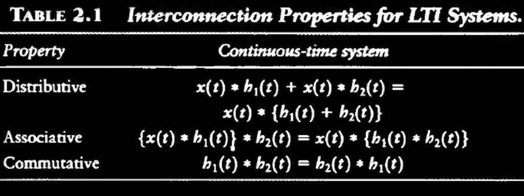
3 2.6 Interconnections of LTl Systems Parallel Connection of LTI Systems Consider two LTI systems with impulse responses h 1 (t) and h 2 (t) connected in parallel, as illustrated in Fig. 2.18(a), the output of this connection of systems, y(t), is the sum of the outputs of the two systems: y t = y 1 t + y 2 t = x t h 1 t + x t h 2 t = Substituting, we get y t = න x τ h 1 (t τ)dτ + න x τ h 2 (t τ)dτ = න x τ h(t τ)dτ Where h (t- ) =h 1 (t- )+ h 2 (t- ), is the impulse response of the equivalent system. 3
 Parallel connection of two systems.")
4 Figure 2.18 (p. 128) Interconnection of two LTI systems. (a) Parallel connection of two systems. (b) Equivalent system. 4
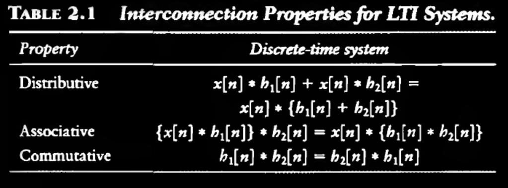
5 Identical results hold for the discrete-time case: x n h 1 + x n h 2 = x n h 1 [n] + h 2 [n] (2.16) 5
6 2.6.2 Cascade Connection of Systems Consider the cascade connection of two LTI systems, as illustrated in Fig. 2.19(a). Let z(t) be the output of the first system and therefore the input to the second system in the cascade. The output is expressed in terms of z(t) as y t = z t h 2 (t) (2.17) Substituting for z(t), we get Putting for z(t), we get y t = න z τ h 2 t τ dτ y t = ඵ x v h 1 τ v h 2 (t τ)dvdτ = න *see Fig b x v h t τ dv = h t h(t) 6
 Cascade connection of two systems. (b) Equivalent system.")
7 Figure 2.19 (p. 128) Interconnection of two LTI systems. (a) Cascade connection of two systems. (b) Equivalent system. (c) Equivalent system: Interchange system order. 7
8 8
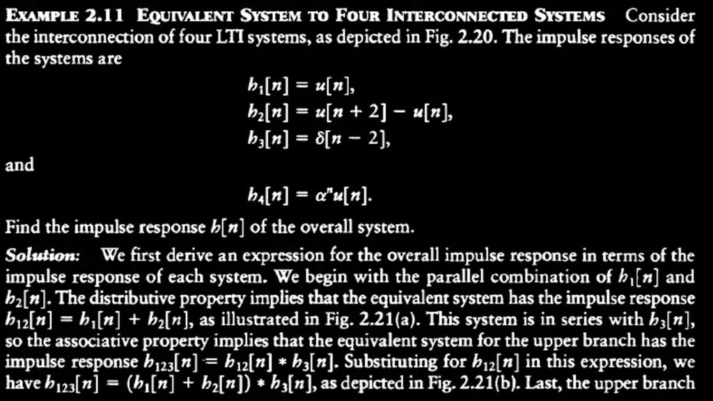
 Interconnection of systems")
9 Figure 2.20 (p. 131) Interconnection of systems for Example
10 10
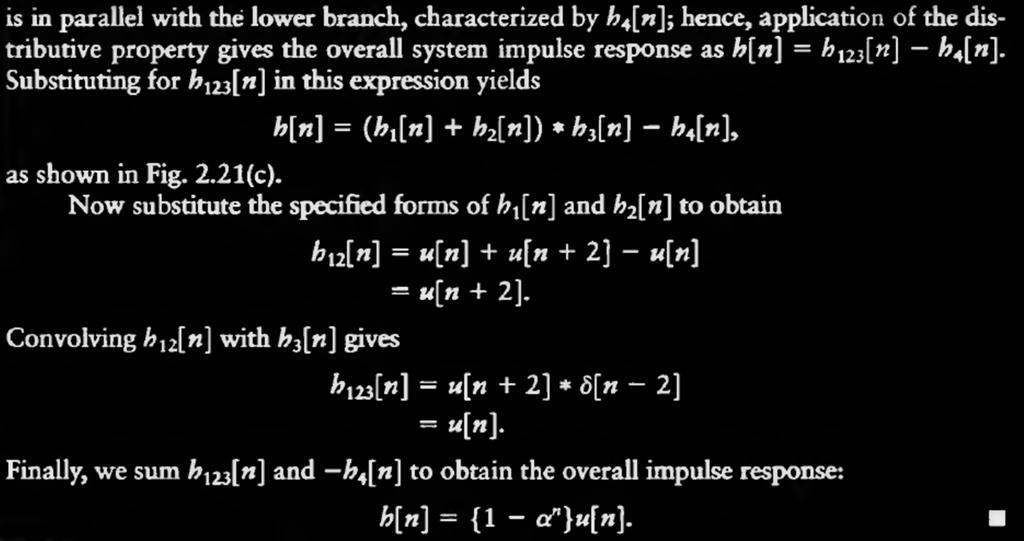
 Reduction of cascade of systems in upper branch of Fig. 2.21(a). (c) Reduction of parallel combination of systems in Fig. 2.21(b) to obtain an equivalent system for Fig.")
11 Figure 2.21 (p. 131) (a) Reduction of parallel combination of LTI systems in upper branch of Fig (b) Reduction of cascade of systems in upper branch of Fig. 2.21(a). (c) Reduction of parallel combination of systems in Fig. 2.21(b) to obtain an equivalent system for Fig
 to the output y(t) for the system")
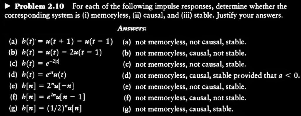
12 Problem 2.8 Find the expression for the impulse response relating the input x(t) to the output y(t) for the system depicted in Fig Answer: Figure 2.22 (p. 132) Interconnection of LTI systems for Problem
13 13
14 14
15 2.7 Relations between LTI System Properties and the Impulse Response Properties of the LTI system, such as memory, causality, and stability, are related to the system s impulse response. Here, we explore these Memoryless LTI Systems The output of a memoryless LTI system depends only on the current input. Exploiting the commutative property of convolution, we may express the output of a discrete-time LTI system as: Expanding, we have y n = h n x n = h k x[n k] k= 15
16 y n = + h 2 x n h 1 x n + 1 +h 0 x n + h 1 x n 1 + h 2 x n 2 (2.27) For this system to be memoryless, y[n] must depend only on x[n] and therefore cannot depend on x[n - k] for k 0. Thus a discrete-time LTI system is memoryless iff h[k] = c [k], c is constant. For continous-time syste, h( ) = c ( ) 16
17 2.7.2 Causal LTI Systems Output of a causal LTI system depends only on past or present values of the input. y n = + h 2 x n h 1 x n + 1 +h 0 x n + h 1 x n 1 + h 2 x n 2 (2.27) For this system to be memoryless, y[n] must depend only on x[n] and therefore In order, then, for y[n] to depend only on past or present values of the input, we require that h[k] = 0 for k < 0. And the convolution sum becomes y n = h k x[n k] For continus time systems k= y t = න h τ x t τ dτ 17
18 2.7.3 Stable LTI Systems We recall from Section that a system is bounded input-bounded output (BIBO) stable if the output is guaranteed to be bounded for every bounded input. Formally, the conditions on h[n] that guarantee stability is given by y[n] = h n x[n] y n = k= h k x[n k] The impulse response of a stable discrete-time LTI system satisfies and for continuous systems, k= y t = න h k < h τ dτ < 18
19 19
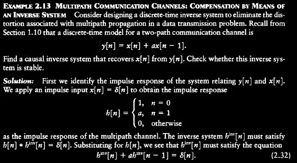
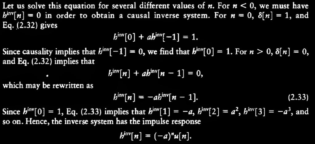
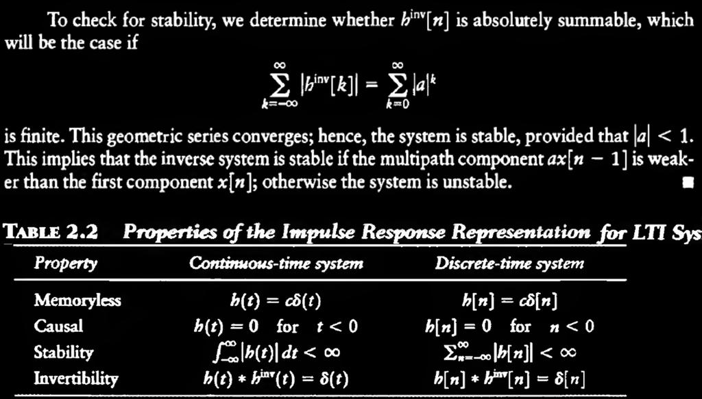
20 2.7.4 Invertible Systems and Deconvolution A system is invertible if the input to the system can be recovered from the output except for a constant scale factor The process of recovering x(t) from h(t)*x(t) is termed deconvolution, since it corresponds to reversing or undoing the convolution operation An inverse system performs deconvolution as shown in Fig Equalization of the distortion introduced by over telephone lines is an example Equalizer reverses distortion and permits much higher data rates to be achieved To derive the relationship between the impulse response of an LTI system, h(t), and that of the corresponding inverse system, h inv (t), we have x t h t h inv t = x t h t h inv t = (t) (2.30) 20
21 For a discrete-time LTI system h[n] h inv [n] = [n] (2.31) Figure 2.24 (p. 137) Cascade of LTI system with impulse response h(t) and inverse system with impulse response h -1 (t). 21
 Interconnection of LTI systems")
22 Figure 2.23 (p. 132) Interconnection of LTI systems for Problem
23 23
24 24
25 25
26 2.8 Step Response Step input signals are often used to characterize the response of an LTI system to sudden changes in the input s n = h n u n = σ k= h k u n k = σ k= h k since u[n-k] = 0 for k > n Similarly, for continous-time systems, we have t s t = n h τ dτ (2.34) 26

, we obtain t 1 s t = න RC e RC u( ) dτ Simplifying, we get: Figure 2.")
27 Example 2.14 RC Circuit: Step Response As shown in Example 1.21, the impulse response of the RC circuit depicted in Fig is h t = 1 t RCu(t) RC e Find the step response of the circuit. Solution: Step represents a switch turning on a constant voltage source at t = 0. Capacitor voltage increases toward the value of source in an exponential manner. Applying (2.34), we obtain t 1 s t = න RC e RC u( ) dτ Simplifying, we get: Figure 2.25 depicts the RC circuit step response for RC = 1 s. 27
 RC circuit step response")
28 Figure 2.25 (p. 140) RC circuit step response for RC = 1 s. 28
29 2.9 Differential and Difference Equation Representations ofltl Systems Difference equations are used to represent discrete-time systems, while differential equations represent continuous-time systems. The general form of a linear constant-coefficient differential equation is σ N d k=0 a k k y t = σ M d dt k k=0 b k k dtk x t (2.35) where a k and b k are constants, x(t) is input and y(t) is the output. A linear constant-coefficient difference equation with derivatives replaced by delayed values of the input x[n] and output y[n]: σ N k=0 a k y[n k] = σ M k=0 b k x[n k] (2.36) 29
 and the output current, y(t), then summing voltage drops around the loop gives Difference equations are easily rearranged")
30 As an example, consider the RLC circuit in Fig with input voltage source x(t) and the output current, y(t), then summing voltage drops around the loop gives Difference equations are easily rearranged to obtain recursive formulas for computing current output from input signal and past outputs from (2.36): 30
 Example of an RLC circuit described by")
31 Figure 2.26 (p. 141) Example of an RLC circuit described by a differential equation. 31
![Computing y[n] for n > 0 from x[n] for second-order difference equation (2.37), (2.](/docs-images/96/129037018/images/32-1.jpg "38) Begin with n = 0, we may determine output by evaluating sequence of equations Output computed from input and past values of output.")
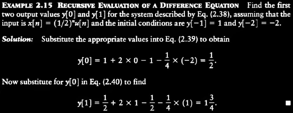
32 Computing y[n] for n > 0 from x[n] for second-order difference equation (2.37), (2.38) Begin with n = 0, we may determine output by evaluating sequence of equations Output computed from input and past values of output. To begin calculation at time n=0, we must know 2 recent past values of output, y[-1], y[-2], known as initial conditions 32
33 33
34 34
: RL circuit.")
35 Figure 2.29 (p. 146): RL circuit. 35
36 2.10 Solving Differential and Difference Equations The output of a system described by a differential or difference equation may be expressed as the sum of two components. 1st is solution of differential or difference equation, called homogeneous solution denote by y (h) 2nd is solution of the original equation, which we term as particular solution and denote by y (p) Thus, the complete solution is y = y (h) + y (p), with the arguments t or n omitted 36
37 The Homogeneous Solution The homogeneous form of a differential or difference equation is obtained by setting all terms involving the input to zero and solving for the homogeneous equation for y (h) (t), N k=0 a k d k dt k y h t = The Particular Solution The particular solution y (p) represents any solution of differential or difference equation for given input. If input is x[n] = A cos( n + ), we assume general sinusoidal response of form y (p) n = c 1 cos( n) +c 1 sin( n), where c 1 and c 2 are determined from y (p) [n] 37
38 The Complete Solution The complete solution of the differential or difference equation is obtained by summing the particular solution and the homogeneous solution finding the unspecified coefficients in the homogeneous solution so that the complete solution satisfies the prescribed initial conditions 38
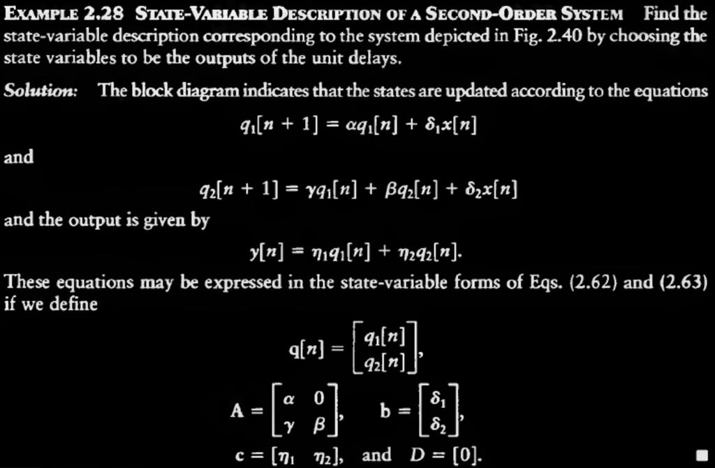
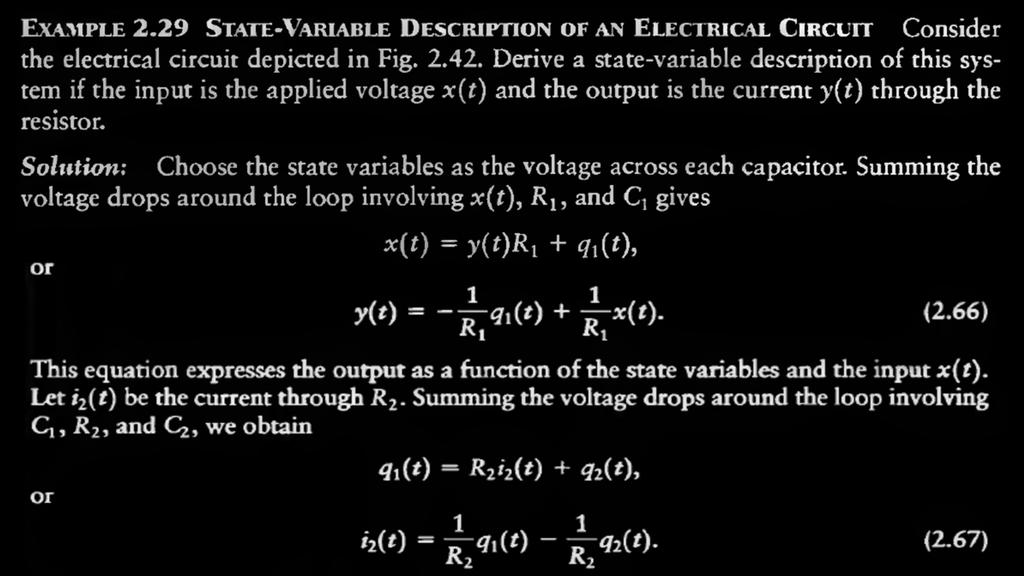
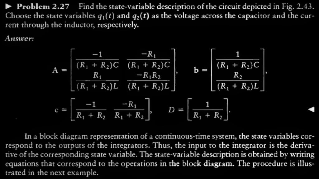
39 2.13 State-Variable Descriptions ofltl Systems The state of a system may be defined as a minimal set of signals that represent the system s entire memory of the past. That is, given only the value of the state at an initial point in time, n i, (or t i ), and the input for times, n > n i, (or t > t i ), we can determine the output for all times n > n i, (or t > t i ) There are many possible state-variable descriptions corresponding to a system with a given input-output characteristic 39
40 The State-Variable Description We shall develop the general state-variable description by starting with the direct form II implementation of a second-order LTI system, depicted in Fig In order to determine output of the system for n n i, we need the input for n n i, and the outputs of the time-shift operations labeled q 1 [n] and q 2 [n] at time n = n i. This suggests that we may choose q 1 [n] and q 2 [n] as the state of the system. Since q 1 [n] and q 2 [n] are outputs of time-shift operations, next value of the state, q 1 [n + 1] and q 2 [n + 1], must correspond to variables at input to time-shift operations The block diagram indicates that the next value of the state is obtained from the current state and the input via the two equations and q 1 n + 1 = a 1 q 1 n + a 2 q 2 n + x[n] (2.57) q 2 [n + 1] = q 1 [n] (2.58) 40
 Direct form II representation of a second-order discrete-time LTI")
41 Figure 2.39 (p. 167) Direct form II representation of a second-order discrete-time LTI system depicting state variables q 1 [n] and q 2 [n]. 41
![The block diagram also indicates that the system output is expressed in terms of the input and the state of the system as Or y[n] = x[n] a 1 q 1 [n] - a 2 q 2 [n] + b 1 q 1](/docs-images/96/129037018/images/42-1.jpg "[n] + b 2 q 2 [n] y[n] = (b 1 a 1 )q 1 [n] (b 2 - a 2 )q 2 [n] + x[n] (2.59) We write Eqs. (2.57) and (2.58) in matrix form as (2.60) while Eq. (2.59) is expressed as (2.")
42 The block diagram also indicates that the system output is expressed in terms of the input and the state of the system as Or y[n] = x[n] a 1 q 1 [n] - a 2 q 2 [n] + b 1 q 1 [n] + b 2 q 2 [n] y[n] = (b 1 a 1 )q 1 [n] (b 2 - a 2 )q 2 [n] + x[n] (2.59) We write Eqs. (2.57) and (2.58) in matrix form as (2.60) while Eq. (2.59) is expressed as (2.61) 42
 and (2.")
![61) as q[n + 1] = Aq[n] + bx[n] (2.](/docs-images/96/129037018/images/43-1.jpg "62) and y[n] = cq[n] + Dx[n] (2.")
43 If we define the state vector as the column vector Then we can rewrite Eqs. (2.60) and (2.61) as q[n + 1] = Aq[n] + bx[n] (2.62) and y[n] = cq[n] + Dx[n] (2.63) where matrix A, vectors b and c, and scalar D are given by 43
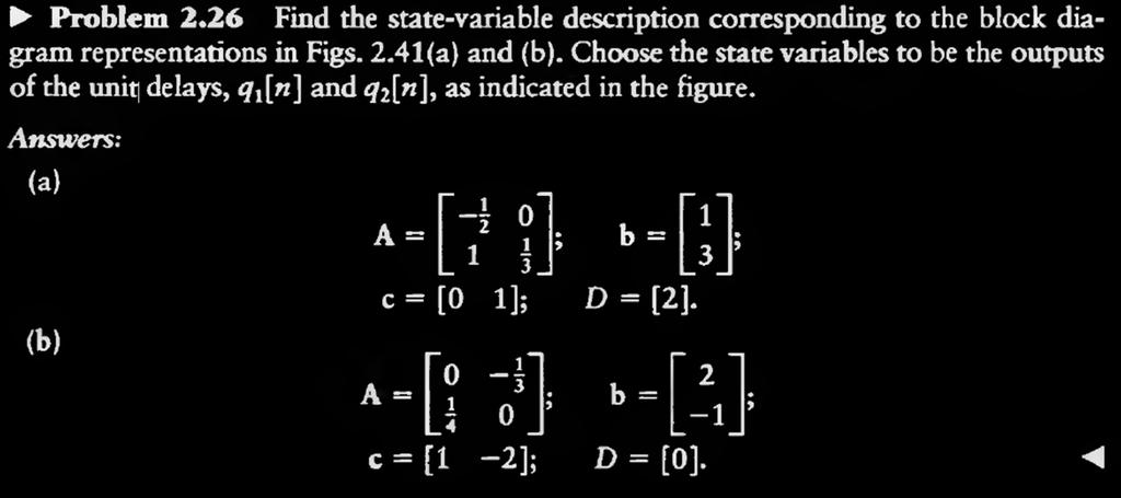
44 Equations (2.62) and (2.63) are general form of a state-variable description corresponding to a discrete-time system Matrix A, vectors b and c, and scalar D represent another description of system Thus, the state-variable description is used in any problem in which the internal system structure needs to be considered If the input-output characteristics of the system are described by an N th -order difference equation, then the state vector q[n] is N by 1, A is N by N, b is N by 1, and c is 1 by N Recall that solving of the difference equation requires N initial conditions, which represent the system s memory of the past, as does the N-dimensional state vector Also, an N th -order system contains at least N time-shift operations in its block diagram representation. 44
45 45
: Block diagram of LTI system for Example")
46 Figure 2.40 (p. 169): Block diagram of LTI system for Example δ 1 γ α ηδ 1 δ 2 η 2 β 46
47 47
 Block diagram of LTI system for Problem 2.26 (2.")
48 Figure 2.41a (p. 170) Block diagram of LTI system for Problem 2.26 (2.41b on next slide). Figure 2.41b (p. 170) 48
49 The state-variable description of continuous-time systems is analogous to that of discrete-time systems, with the exception that the state equation given by (2.62) is expressed in terms of a derivative, i.e. and d dt q t = Aq t + bx(t) (2.64) y t = cq t + Dx(t) (2.64) Matrix A, vectors b and c, and scalar D describe the internal structure of system State variables are usually chosen as the physical quantities associated with such devices. For example, in electrical systems, the energy storage devices are capacitors and inductors. Accordingly, we may choose state variables to correspond to the voltages across capacitors or the currents through inductors 49
50 50
51 Figure 2.42 (p. 171): Circuit diagram of LTI system for Example
52 52
53 53
54 54
 Circuit diagram of LTI system")
55 Figure 2.43 (p. 173) Circuit diagram of LTI system for Problem
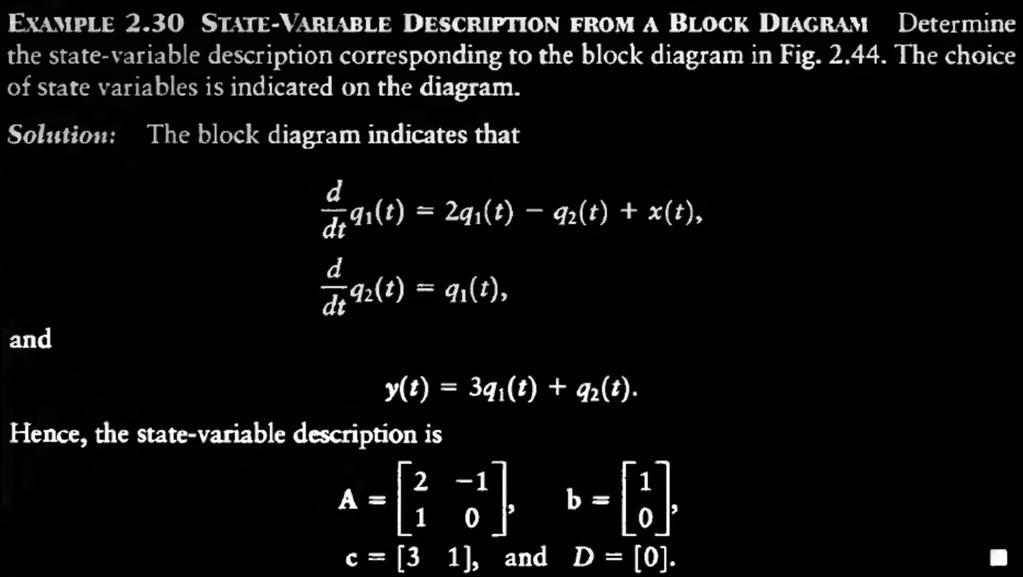
 Block diagram of LTI system")
56 Figure 2.44 (p. 172) Block diagram of LTI system for Example
57 57

58 Transformations of the State Different state-variable descriptions are obtained by transforming state variables The transformation is accomplished by defining a new set of state variables that are a weighted sum of the original ones This changes the form of A, b, c, and D, but does not change the input-output characteristics of the system To illustrate the procedure, consider Example 2.30 again. Let us define new states q 2 (t)= q 1 (t) and q 1 (t )= q 2 (t) Here, we simply have interchanged the state variables: q 2 (t) is the output of the first integrator and q 1 (t ) is the output of the second integrator The state-variable description is 58
59 End of Chapter 2 Please prepare for the next quiz on Chapter 2 59
60 Figure 2.45 (p. 177) Convolution sum computed using MATLAB. 60
61 Figure 2.46 (p. 177) Solution to Problem
62 Figure 2.47 (p. 178) Step response computed using MATLAB. 62
63 Figure 2.48 (p. 181) Impulse responses associated with the original and transformed state-variable descriptions computer using MATLAB. 63
64 Figure P2.32 (p. 183) 64
65 Figure P2.34 (p. 184) 65
66 Figure P2.38 (p. 185) 66
67 Figure P2.40 (p. 186)
68 Figure P2.41 (p. 187) 68
69 Figure P2.43 (p. 187) 69
70 Figure P2.46 (p. 188) 70
71 Figure P2.52 (p. 188) 71
72 Figure P2.61 (p. 189) 72
73 Figure P2.65 (p. 190) 73
74 Figure P2.68 (p. 190) 74
75 Figure P2.69 (p. 190) 75
76 Figure P2.71 (p. 191) 76
77 Figure P2.74 (p. 192) 77
78 Figure P2.75 (p. 192) 78
79 Figure P2.81 (p. 194) 79
Chapter 2 Time-Domain Representations of LTI Systems
 Chapter 2 Time-Domain Representations of LTI Systems 1 Introduction Impulse responses of LTI systems Linear constant-coefficients differential or difference equations of LTI systems Block diagram representations
Chapter 2: Time-Domain Representations of Linear Time-Invariant Systems. Chih-Wei Liu
 Chapter : Time-Domain Representations of Linear Time-Invariant Systems Chih-Wei Liu Outline Characteristics of Systems Described by Differential and Difference Equations Block Diagram Representations State-Variable
Cosc 3451 Signals and Systems. What is a system? Systems Terminology and Properties of Systems
 Cosc 3451 Signals and Systems Systems Terminology and Properties of Systems What is a system? an entity that manipulates one or more signals to yield new signals (often to accomplish a function) can be
Chapter 3 Convolution Representation
 Chapter 3 Convolution Representation DT Unit-Impulse Response Consider the DT SISO system: xn [ ] System yn [ ] xn [ ] = δ[ n] If the input signal is and the system has no energy at n = 0, the output yn
Properties of LTI Systems
 Properties of LTI Systems Properties of Continuous Time LTI Systems Systems with or without memory: A system is memory less if its output at any time depends only on the value of the input at that same
1.4 Unit Step & Unit Impulse Functions
 1.4 Unit Step & Unit Impulse Functions 1.4.1 The Discrete-Time Unit Impulse and Unit-Step Sequences Unit Impulse Function: δ n = ቊ 0, 1, n 0 n = 0 Figure 1.28: Discrete-time Unit Impulse (sample) 1 [n]
信號與系統 Signals and Systems
 Spring 2010 信號與系統 Signals and Systems Chapter SS-2 Linear Time-Invariant Systems Feng-Li Lian NTU-EE Feb10 Jun10 Figures and images used in these lecture notes are adopted from Signals & Systems by Alan
Signals and Systems Chapter 2
 Signals and Systems Chapter 2 Continuous-Time Systems Prof. Yasser Mostafa Kadah Overview of Chapter 2 Systems and their classification Linear time-invariant systems System Concept Mathematical transformation
信號與系統 Signals and Systems
 Spring 2015 信號與系統 Signals and Systems Chapter SS-2 Linear Time-Invariant Systems Feng-Li Lian NTU-EE Feb15 Jun15 Figures and images used in these lecture notes are adopted from Signals & Systems by Alan
Lecture 2 Discrete-Time LTI Systems: Introduction
 Lecture 2 Discrete-Time LTI Systems: Introduction Outline 2.1 Classification of Systems.............................. 1 2.1.1 Memoryless................................. 1 2.1.2 Causal....................................
Differential and Difference LTI systems
 Signals and Systems Lecture: 6 Differential and Difference LTI systems Differential and difference linear time-invariant (LTI) systems constitute an extremely important class of systems in engineering.
ECE 301 Division 1 Exam 1 Solutions, 10/6/2011, 8-9:45pm in ME 1061.
 ECE 301 Division 1 Exam 1 Solutions, 10/6/011, 8-9:45pm in ME 1061. Your ID will be checked during the exam. Please bring a No. pencil to fill out the answer sheet. This is a closed-book exam. No calculators
Chap 2. Discrete-Time Signals and Systems
 Digital Signal Processing Chap 2. Discrete-Time Signals and Systems Chang-Su Kim Discrete-Time Signals CT Signal DT Signal Representation 0 4 1 1 1 2 3 Functional representation 1, n 1,3 x[ n] 4, n 2 0,
EE 210. Signals and Systems Solutions of homework 2
 EE 2. Signals and Systems Solutions of homework 2 Spring 2 Exercise Due Date Week of 22 nd Feb. Problems Q Compute and sketch the output y[n] of each discrete-time LTI system below with impulse response
2. CONVOLUTION. Convolution sum. Response of d.t. LTI systems at a certain input signal
 2. CONVOLUTION Convolution sum. Response of d.t. LTI systems at a certain input signal Any signal multiplied by the unit impulse = the unit impulse weighted by the value of the signal in 0: xn [ ] δ [
Ch 2: Linear Time-Invariant System
 Ch 2: Linear Time-Invariant System A system is said to be Linear Time-Invariant (LTI) if it possesses the basic system properties of linearity and time-invariance. Consider a system with an output signal
University Question Paper Solution
 Unit 1: Introduction University Question Paper Solution 1. Determine whether the following systems are: i) Memoryless, ii) Stable iii) Causal iv) Linear and v) Time-invariant. i) y(n)= nx(n) ii) y(t)=
Digital Signal Processing Lecture 3 - Discrete-Time Systems
 Digital Signal Processing - Discrete-Time Systems Electrical Engineering and Computer Science University of Tennessee, Knoxville August 25, 2015 Overview 1 2 3 4 5 6 7 8 Introduction Three components of
NAME: 23 February 2017 EE301 Signals and Systems Exam 1 Cover Sheet
 NAME: 23 February 2017 EE301 Signals and Systems Exam 1 Cover Sheet Test Duration: 75 minutes Coverage: Chaps 1,2 Open Book but Closed Notes One 85 in x 11 in crib sheet Calculators NOT allowed DO NOT
x(t) = t[u(t 1) u(t 2)] + 1[u(t 2) u(t 3)]
![x(t) = t[u(t 1) u(t 2)] + 1[u(t 2) u(t 3)]](/thumbs/96/128551587.jpg "x(t) = t[u(t 1) u(t 2)] + 1[u(t 2) u(t 3)]") ECE30 Summer II, 2006 Exam, Blue Version July 2, 2006 Name: Solution Score: 00/00 You must show all of your work for full credit. Calculators may NOT be used.. (5 points) x(t) = tu(t ) + ( t)u(t 2) u(t
ECE30 Summer II, 2006 Exam, Blue Version July 2, 2006 Name: Solution Score: 00/00 You must show all of your work for full credit. Calculators may NOT be used.. (5 points) x(t) = tu(t ) + ( t)u(t 2) u(t
Lecture 2. Introduction to Systems (Lathi )
") Lecture 2 Introduction to Systems (Lathi 1.6-1.8) Pier Luigi Dragotti Department of Electrical & Electronic Engineering Imperial College London URL: www.commsp.ee.ic.ac.uk/~pld/teaching/ E-mail: p.dragotti@imperial.ac.uk
Lecture 2 Introduction to Systems (Lathi 1.6-1.8) Pier Luigi Dragotti Department of Electrical & Electronic Engineering Imperial College London URL: www.commsp.ee.ic.ac.uk/~pld/teaching/ E-mail: p.dragotti@imperial.ac.uk
Analog Signals and Systems and their properties
 Analog Signals and Systems and their properties Main Course Objective: Recall course objectives Understand the fundamentals of systems/signals interaction (know how systems can transform or filter signals)
Digital Signal Processing Lecture 5
 Remote Sensing Laboratory Dept. of Information Engineering and Computer Science University of Trento Via Sommarive, 14, I-38123 Povo, Trento, Italy Digital Signal Processing Lecture 5 Begüm Demir E-mail:
Lecture 7: Laplace Transform and Its Applications Dr.-Ing. Sudchai Boonto
 Dr-Ing Sudchai Boonto Department of Control System and Instrumentation Engineering King Mongkut s Unniversity of Technology Thonburi Thailand Outline Motivation The Laplace Transform The Laplace Transform
QUESTION BANK SIGNALS AND SYSTEMS (4 th SEM ECE)
") QUESTION BANK SIGNALS AND SYSTEMS (4 th SEM ECE) 1. For the signal shown in Fig. 1, find x(2t + 3). i. Fig. 1 2. What is the classification of the systems? 3. What are the Dirichlet s conditions of Fourier
QUESTION BANK SIGNALS AND SYSTEMS (4 th SEM ECE) 1. For the signal shown in Fig. 1, find x(2t + 3). i. Fig. 1 2. What is the classification of the systems? 3. What are the Dirichlet s conditions of Fourier
Chapter 1 Fundamental Concepts
 Chapter 1 Fundamental Concepts Signals A signal is a pattern of variation of a physical quantity as a function of time, space, distance, position, temperature, pressure, etc. These quantities are usually
EE 341 Homework Chapter 2
 EE 341 Homework Chapter 2 2.1 The electrical circuit shown in Fig. P2.1 consists of two resistors R1 and R2 and a capacitor C. Determine the differential equation relating the input voltage v(t) to the
III. Time Domain Analysis of systems
 1 III. Time Domain Analysis of systems Here, we adapt properties of continuous time systems to discrete time systems Section 2.2-2.5, pp 17-39 System Notation y(n) = T[ x(n) ] A. Types of Systems Memoryless
New Mexico State University Klipsch School of Electrical Engineering. EE312 - Signals and Systems I Spring 2018 Exam #1
 New Mexico State University Klipsch School of Electrical Engineering EE312 - Signals and Systems I Spring 2018 Exam #1 Name: Prob. 1 Prob. 2 Prob. 3 Prob. 4 Total / 30 points / 20 points / 25 points /
LTI Systems (Continuous & Discrete) - Basics
 - Basics") LTI Systems (Continuous & Discrete) - Basics 1. A system with an input x(t) and output y(t) is described by the relation: y(t) = t. x(t). This system is (a) linear and time-invariant (b) linear and time-varying
LTI Systems (Continuous & Discrete) - Basics 1. A system with an input x(t) and output y(t) is described by the relation: y(t) = t. x(t). This system is (a) linear and time-invariant (b) linear and time-varying
Lecture 1 From Continuous-Time to Discrete-Time
 Lecture From Continuous-Time to Discrete-Time Outline. Continuous and Discrete-Time Signals and Systems................. What is a signal?................................2 What is a system?.............................
ECE 314 Signals and Systems Fall 2012
 ECE 31 ignals and ystems Fall 01 olutions to Homework 5 Problem.51 Determine the impulse response of the system described by y(n) = x(n) + ax(n k). Replace x by δ to obtain the impulse response: h(n) =
06/12/ rws/jMc- modif SuFY10 (MPF) - Textbook Section IX 1
 - Textbook Section IX 1") IV. Continuous-Time Signals & LTI Systems [p. 3] Analog signal definition [p. 4] Periodic signal [p. 5] One-sided signal [p. 6] Finite length signal [p. 7] Impulse function [p. 9] Sampling property [p.11]
IV. Continuous-Time Signals & LTI Systems [p. 3] Analog signal definition [p. 4] Periodic signal [p. 5] One-sided signal [p. 6] Finite length signal [p. 7] Impulse function [p. 9] Sampling property [p.11]
Module 1: Signals & System
 Module 1: Signals & System Lecture 6: Basic Signals in Detail Basic Signals in detail We now introduce formally some of the basic signals namely 1) The Unit Impulse function. 2) The Unit Step function
2 Classification of Continuous-Time Systems
 Continuous-Time Signals and Systems 1 Preliminaries Notation for a continuous-time signal: x(t) Notation: If x is the input to a system T and y the corresponding output, then we use one of the following
The Convolution Sum for Discrete-Time LTI Systems
 The Convolution Sum for Discrete-Time LTI Systems Andrew W. H. House 01 June 004 1 The Basics of the Convolution Sum Consider a DT LTI system, L. x(n) L y(n) DT convolution is based on an earlier result
New Mexico State University Klipsch School of Electrical Engineering. EE312 - Signals and Systems I Fall 2017 Exam #1
 New Mexico State University Klipsch School of Electrical Engineering EE312 - Signals and Systems I Fall 2017 Exam #1 Name: Prob. 1 Prob. 2 Prob. 3 Prob. 4 Total / 30 points / 20 points / 25 points / 25
Examples. 2-input, 1-output discrete-time systems: 1-input, 1-output discrete-time systems:
 Discrete-Time s - I Time-Domain Representation CHAPTER 4 These lecture slides are based on "Digital Signal Processing: A Computer-Based Approach, 4th ed." textbook by S.K. Mitra and its instructor materials.
Noise - irrelevant data; variability in a quantity that has no meaning or significance. In most cases this is modeled as a random variable.
 1.1 Signals and Systems Signals convey information. Systems respond to (or process) information. Engineers desire mathematical models for signals and systems in order to solve design problems efficiently
Classification of Discrete-Time Systems. System Properties. Terminology: Implication. Terminology: Equivalence
 Classification of Discrete-Time Systems Professor Deepa Kundur University of Toronto Why is this so important? mathematical techniques developed to analyze systems are often contingent upon the general
Quiz. Good luck! Signals & Systems ( ) Number of Problems: 19. Number of Points: 19. Permitted aids:
 Number of Problems: 19. Number of Points: 19. Permitted aids:") Quiz November th, Signals & Systems (--) Prof. R. D Andrea Quiz Exam Duration: Min Number of Problems: Number of Points: Permitted aids: Important: None Questions must be answered on the provided answer
Quiz November th, Signals & Systems (--) Prof. R. D Andrea Quiz Exam Duration: Min Number of Problems: Number of Points: Permitted aids: Important: None Questions must be answered on the provided answer
Lecture 19 IIR Filters
 Lecture 19 IIR Filters Fundamentals of Digital Signal Processing Spring, 2012 Wei-Ta Chu 2012/5/10 1 General IIR Difference Equation IIR system: infinite-impulse response system The most general class
ECE 301 Fall 2011 Division 1 Homework 5 Solutions
 ECE 301 Fall 2011 ivision 1 Homework 5 Solutions Reading: Sections 2.4, 3.1, and 3.2 in the textbook. Problem 1. Suppose system S is initially at rest and satisfies the following input-output difference
Lecture 2 ELE 301: Signals and Systems
 Lecture 2 ELE 301: Signals and Systems Prof. Paul Cuff Princeton University Fall 2011-12 Cuff (Lecture 2) ELE 301: Signals and Systems Fall 2011-12 1 / 70 Models of Continuous Time Signals Today s topics:
Signals and Systems. VTU Edusat program. By Dr. Uma Mudenagudi Department of Electronics and Communication BVCET, Hubli
 Signals and Systems Course material VTU Edusat program By Dr. Uma Mudenagudi uma@bvb.edu Department of Electronics and Communication BVCET, Hubli-580030 May 22, 2009 Contents 1 Introduction 1 1.1 Class
Chapter 1 Fundamental Concepts
 Chapter 1 Fundamental Concepts 1 Signals A signal is a pattern of variation of a physical quantity, often as a function of time (but also space, distance, position, etc). These quantities are usually the
e st f (t) dt = e st tf(t) dt = L {t f(t)} s
 dt = e st tf(t) dt = L {t f(t)} s") Additional operational properties How to find the Laplace transform of a function f (t) that is multiplied by a monomial t n, the transform of a special type of integral, and the transform of a periodic
Additional operational properties How to find the Laplace transform of a function f (t) that is multiplied by a monomial t n, the transform of a special type of integral, and the transform of a periodic
Analog vs. discrete signals
 Analog vs. discrete signals Continuous-time signals are also known as analog signals because their amplitude is analogous (i.e., proportional) to the physical quantity they represent. Discrete-time signals
EE Homework 5 - Solutions
 EE054 - Homework 5 - Solutions 1. We know the general result that the -transform of α n 1 u[n] is with 1 α 1 ROC α < < and the -transform of α n 1 u[ n 1] is 1 α 1 with ROC 0 < α. Using this result, the
CH.3 Continuous-Time Linear Time-Invariant System
 CH.3 Continuous-Time Linear Time-Invariant System 1 LTI System Characterization 1.1 what does LTI mean? In Ch.2, the properties of the system are investigated. We are particularly interested in linear
Introduction to Signals and Systems Lecture #4 - Input-output Representation of LTI Systems Guillaume Drion Academic year
 Introduction to Signals and Systems Lecture #4 - Input-output Representation of LTI Systems Guillaume Drion Academic year 2017-2018 1 Outline Systems modeling: input/output approach of LTI systems. Convolution
1.17 : Consider a continuous-time system with input x(t) and output y(t) related by y(t) = x( sin(t)).
 and output y(t) related by y(t) = x( sin(t)).") (Note: here are the solution, only showing you the approach to solve the problems. If you find some typos or calculation error, please post it on Piazza and let us know ).7 : Consider a continuous-time
(Note: here are the solution, only showing you the approach to solve the problems. If you find some typos or calculation error, please post it on Piazza and let us know ).7 : Consider a continuous-time
Review of Frequency Domain Fourier Series: Continuous periodic frequency components
 Today we will review: Review of Frequency Domain Fourier series why we use it trig form & exponential form how to get coefficients for each form Eigenfunctions what they are how they relate to LTI systems
To find the step response of an RC circuit
 To find the step response of an RC circuit v( t) v( ) [ v( t) v( )] e tt The time constant = RC The final capacitor voltage v() The initial capacitor voltage v(t ) To find the step response of an RL circuit
Digital Signal Processing Lecture 4
 Remote Sensing Laboratory Dept. of Information Engineering and Computer Science University of Trento Via Sommarive, 14, I-38123 Povo, Trento, Italy Digital Signal Processing Lecture 4 Begüm Demir E-mail:
VU Signal and Image Processing
 052600 VU Signal and Image Processing Torsten Möller + Hrvoje Bogunović + Raphael Sahann torsten.moeller@univie.ac.at hrvoje.bogunovic@meduniwien.ac.at raphael.sahann@univie.ac.at vda.cs.univie.ac.at/teaching/sip/18s/
DEPARTMENT OF ELECTRICAL AND ELECTRONIC ENGINEERING EXAMINATIONS 2010
 [E2.5] IMPERIAL COLLEGE LONDON DEPARTMENT OF ELECTRICAL AND ELECTRONIC ENGINEERING EXAMINATIONS 2010 EEE/ISE PART II MEng. BEng and ACGI SIGNALS AND LINEAR SYSTEMS Time allowed: 2:00 hours There are FOUR
Question Paper Code : AEC11T02
 Hall Ticket No Question Paper Code : AEC11T02 VARDHAMAN COLLEGE OF ENGINEERING (AUTONOMOUS) Affiliated to JNTUH, Hyderabad Four Year B. Tech III Semester Tutorial Question Bank 2013-14 (Regulations: VCE-R11)
UNIT 1. SIGNALS AND SYSTEM
 Page no: 1 UNIT 1. SIGNALS AND SYSTEM INTRODUCTION A SIGNAL is defined as any physical quantity that changes with time, distance, speed, position, pressure, temperature or some other quantity. A SIGNAL
Problem Value Score No/Wrong Rec 3
 GEORGIA INSTITUTE OF TECHNOLOGY SCHOOL of ELECTRICAL & COMPUTER ENGINEERING QUIZ #3 DATE: 21-Nov-11 COURSE: ECE-2025 NAME: GT username: LAST, FIRST (ex: gpburdell3) 3 points 3 points 3 points Recitation
Professor Fearing EECS120/Problem Set 2 v 1.01 Fall 2016 Due at 4 pm, Fri. Sep. 9 in HW box under stairs (1st floor Cory) Reading: O&W Ch 1, Ch2.
 Reading: O&W Ch 1, Ch2.") Professor Fearing EECS120/Problem Set 2 v 1.01 Fall 20 Due at 4 pm, Fri. Sep. 9 in HW box under stairs (1st floor Cory) Reading: O&W Ch 1, Ch2. Note: Π(t) = u(t + 1) u(t 1 ), and r(t) = tu(t) where u(t)
Professor Fearing EECS120/Problem Set 2 v 1.01 Fall 20 Due at 4 pm, Fri. Sep. 9 in HW box under stairs (1st floor Cory) Reading: O&W Ch 1, Ch2. Note: Π(t) = u(t + 1) u(t 1 ), and r(t) = tu(t) where u(t)
e jωt y (t) = ω 2 Ke jωt K =
 = ω 2 Ke jωt K =") BME 171, Sec 2: Homework 2 Solutions due Tue, Sep 16 by 5pm 1. Consider a system governed by the second-order differential equation a d2 y(t) + b dy(t) where a, b and c are nonnegative real numbers. (a)
BME 171, Sec 2: Homework 2 Solutions due Tue, Sep 16 by 5pm 1. Consider a system governed by the second-order differential equation a d2 y(t) + b dy(t) where a, b and c are nonnegative real numbers. (a)
EEL3135: Homework #4
 EEL335: Homework #4 Problem : For each of the systems below, determine whether or not the system is () linear, () time-invariant, and (3) causal: (a) (b) (c) xn [ ] cos( 04πn) (d) xn [ ] xn [ ] xn [ 5]
EE292: Fundamentals of ECE
 EE292: Fundamentals of ECE Fall 2012 TTh 10:00-11:15 SEB 1242 Lecture 14 121011 http://www.ee.unlv.edu/~b1morris/ee292/ 2 Outline Review Steady-State Analysis RC Circuits RL Circuits 3 DC Steady-State
Final Exam January 31, Solutions
 Final Exam January 31, 014 Signals & Systems (151-0575-01) Prof. R. D Andrea & P. Reist Solutions Exam Duration: Number of Problems: Total Points: Permitted aids: Important: 150 minutes 7 problems 50 points
Solving a RLC Circuit using Convolution with DERIVE for Windows
 Solving a RLC Circuit using Convolution with DERIVE for Windows Michel Beaudin École de technologie supérieure, rue Notre-Dame Ouest Montréal (Québec) Canada, H3C K3 mbeaudin@seg.etsmtl.ca - Introduction
Chapter 2: Linear systems & sinusoids OVE EDFORS DEPT. OF EIT, LUND UNIVERSITY
 Chapter 2: Linear systems & sinusoids OVE EDFORS DEPT. OF EIT, LUND UNIVERSITY Learning outcomes After this lecture, the student should understand what a linear system is, including linearity conditions,
Chapter 5 Frequency Domain Analysis of Systems
 Chapter 5 Frequency Domain Analysis of Systems CT, LTI Systems Consider the following CT LTI system: xt () ht () yt () Assumption: the impulse response h(t) is absolutely integrable, i.e., ht ( ) dt< (this
Module 4. Related web links and videos. 1. FT and ZT
 Module 4 Laplace transforms, ROC, rational systems, Z transform, properties of LT and ZT, rational functions, system properties from ROC, inverse transforms Related web links and videos Sl no Web link
Linear Systems. ! Textbook: Strum, Contemporary Linear Systems using MATLAB.
 Linear Systems LS 1! Textbook: Strum, Contemporary Linear Systems using MATLAB.! Contents 1. Basic Concepts 2. Continuous Systems a. Laplace Transforms and Applications b. Frequency Response of Continuous
ELEN E4810: Digital Signal Processing Topic 2: Time domain
 ELEN E4810: Digital Signal Processing Topic 2: Time domain 1. Discrete-time systems 2. Convolution 3. Linear Constant-Coefficient Difference Equations (LCCDEs) 4. Correlation 1 1. Discrete-time systems
GATE EE Topic wise Questions SIGNALS & SYSTEMS
 www.gatehelp.com GATE EE Topic wise Questions YEAR 010 ONE MARK Question. 1 For the system /( s + 1), the approximate time taken for a step response to reach 98% of the final value is (A) 1 s (B) s (C)
Volterra/Wiener Representation of Non-Linear Systems
 Berkeley Volterra/Wiener Representation of Non-Linear Systems Prof. Ali M. U.C. Berkeley Copyright c 2014 by Ali M. Linear Input/Output Representation A linear (LTI) system is completely characterized
Digital Signal Processing, Homework 1, Spring 2013, Prof. C.D. Chung
 Digital Signal Processing, Homework, Spring 203, Prof. C.D. Chung. (0.5%) Page 99, Problem 2.2 (a) The impulse response h [n] of an LTI system is known to be zero, except in the interval N 0 n N. The input
Module 4 : Laplace and Z Transform Problem Set 4
 Module 4 : Laplace and Z Transform Problem Set 4 Problem 1 The input x(t) and output y(t) of a causal LTI system are related to the block diagram representation shown in the figure. (a) Determine a differential
Discrete-time signals and systems
 Discrete-time signals and systems 1 DISCRETE-TIME DYNAMICAL SYSTEMS x(t) G y(t) Linear system: Output y(n) is a linear function of the inputs sequence: y(n) = k= h(k)x(n k) h(k): impulse response of the
ELEG 305: Digital Signal Processing
 ELEG 305: Digital Signal Processing Lecture 1: Course Overview; Discrete-Time Signals & Systems Kenneth E. Barner Department of Electrical and Computer Engineering University of Delaware Fall 2008 K. E.
EECE 3620: Linear Time-Invariant Systems: Chapter 2
 EECE 3620: Linear Time-Invariant Systems: Chapter 2 Prof. K. Chandra ECE, UMASS Lowell September 7, 2016 1 Continuous Time Systems In the context of this course, a system can represent a simple or complex
School of Engineering Faculty of Built Environment, Engineering, Technology & Design
 Module Name and Code : ENG60803 Real Time Instrumentation Semester and Year : Semester 5/6, Year 3 Lecture Number/ Week : Lecture 3, Week 3 Learning Outcome (s) : LO5 Module Co-ordinator/Tutor : Dr. Phang
Lecture 11 FIR Filters
 Lecture 11 FIR Filters Fundamentals of Digital Signal Processing Spring, 2012 Wei-Ta Chu 2012/4/12 1 The Unit Impulse Sequence Any sequence can be represented in this way. The equation is true if k ranges
3.2 Complex Sinusoids and Frequency Response of LTI Systems
 3. Introduction. A signal can be represented as a weighted superposition of complex sinusoids. x(t) or x[n]. LTI system: LTI System Output = A weighted superposition of the system response to each complex
ECE-202 FINAL April 30, 2018 CIRCLE YOUR DIVISION
 ECE 202 Final, Spring 8 ECE-202 FINAL April 30, 208 Name: (Please print clearly.) Student Email: CIRCLE YOUR DIVISION DeCarlo- 7:30-8:30 DeCarlo-:30-2:45 2025 202 INSTRUCTIONS There are 34 multiple choice
EE123 Digital Signal Processing
 EE123 Digital Signal Processing Lecture 2 Discrete Time Systems Today Last time: Administration Overview Announcement: HW1 will be out today Lab 0 out webcast out Today: Ch. 2 - Discrete-Time Signals and
EE -213 BASIC CIRCUIT ANALYSIS LAB MANUAL
 EE -213 BASIC CIRCUIT ANALYSIS LAB MANUAL EE 213 Fall 2009 LABORATORY #1 INTRODUCTION TO MATLAB INTRODUCTION The purpose of this laboratory is to introduce you to Matlab and to illustrate some of its circuit
Final Exam 14 May LAST Name FIRST Name Lab Time
 EECS 20n: Structure and Interpretation of Signals and Systems Department of Electrical Engineering and Computer Sciences UNIVERSITY OF CALIFORNIA BERKELEY Final Exam 14 May 2005 LAST Name FIRST Name Lab
A system that is both linear and time-invariant is called linear time-invariant (LTI).
.") The Cooper Union Department of Electrical Engineering ECE111 Signal Processing & Systems Analysis Lecture Notes: Time, Frequency & Transform Domains February 28, 2012 Signals & Systems Signals are mapped
The Cooper Union Department of Electrical Engineering ECE111 Signal Processing & Systems Analysis Lecture Notes: Time, Frequency & Transform Domains February 28, 2012 Signals & Systems Signals are mapped
Convolution. Define a mathematical operation on discrete-time signals called convolution, represented by *. Given two discrete-time signals x 1, x 2,
 Filters Filters So far: Sound signals, connection to Fourier Series, Introduction to Fourier Series and Transforms, Introduction to the FFT Today Filters Filters: Keep part of the signal we are interested
Lecture 6: Time-Domain Analysis of Continuous-Time Systems Dr.-Ing. Sudchai Boonto
 Lecture 6: Time-Domain Analysis of Continuous-Time Systems Dr-Ing Sudchai Boonto Department of Control System and Instrumentation Engineering King Mongkut s Unniversity of Technology Thonburi Thailand
Digital Signal Processing BEC505 Chapter 1: Introduction What is a Signal? Signals: The Mathematical Way What is Signal processing?
 Digital Signal Processing BEC505 Chapter 1: Introduction What is a Signal? Anything which carries information is a signal. e.g. human voice, chirping of birds, smoke signals, gestures (sign language),
EE 16B Final, December 13, Name: SID #:
 EE 16B Final, December 13, 2016 Name: SID #: Important Instructions: Show your work. An answer without explanation is not acceptable and does not guarantee any credit. Only the front pages will be scanned
EEE105 Teori Litar I Chapter 7 Lecture #3. Dr. Shahrel Azmin Suandi Emel:
 EEE105 Teori Litar I Chapter 7 Lecture #3 Dr. Shahrel Azmin Suandi Emel: shahrel@eng.usm.my What we have learnt so far? Chapter 7 introduced us to first-order circuit From the last lecture, we have learnt
EE 224 Signals and Systems I Review 1/10
 EE 224 Signals and Systems I Review 1/10 Class Contents Signals and Systems Continuous-Time and Discrete-Time Time-Domain and Frequency Domain (all these dimensions are tightly coupled) SIGNALS SYSTEMS
Lecture V: Linear difference and differential equations
 Lecture V: Linear difference and differential equations BME 171: Signals and Systems Duke University September 10, 2008 This lecture Plan for the lecture: 1 Discrete-time systems linear difference equations
Signals & Systems interaction in the Time Domain. (Systems will be LTI from now on unless otherwise stated)
") Signals & Systems interaction in the Time Domain (Systems will be LTI from now on unless otherwise stated) Course Objectives Specific Course Topics: -Basic test signals and their properties -Basic system
Signals & Systems interaction in the Time Domain (Systems will be LTI from now on unless otherwise stated) Course Objectives Specific Course Topics: -Basic test signals and their properties -Basic system
Digital Filters Ying Sun
 Digital Filters Ying Sun Digital filters Finite impulse response (FIR filter: h[n] has a finite numbers of terms. Infinite impulse response (IIR filter: h[n] has infinite numbers of terms. Causal filter:
Source-Free RC Circuit
 First Order Circuits Source-Free RC Circuit Initial charge on capacitor q = Cv(0) so that voltage at time 0 is v(0). What is v(t)? Prof Carruthers (ECE @ BU) EK307 Notes Summer 2018 150 / 264 First Order
Let H(z) = P(z)/Q(z) be the system function of a rational form. Let us represent both P(z) and Q(z) as polynomials of z (not z -1 )
 = P(z)/Q(z) be the system function of a rational form. Let us represent both P(z) and Q(z) as polynomials of z (not z -1 )") Review: Poles and Zeros of Fractional Form Let H() = P()/Q() be the system function of a rational form. Let us represent both P() and Q() as polynomials of (not - ) Then Poles: the roots of Q()=0 Zeros:
Review: Poles and Zeros of Fractional Form Let H() = P()/Q() be the system function of a rational form. Let us represent both P() and Q() as polynomials of (not - ) Then Poles: the roots of Q()=0 Zeros:
Ch. 7: Z-transform Reading
 c J. Fessler, June 9, 3, 6:3 (student version) 7. Ch. 7: Z-transform Definition Properties linearity / superposition time shift convolution: y[n] =h[n] x[n] Y (z) =H(z) X(z) Inverse z-transform by coefficient
New Mexico State University Klipsch School of Electrical Engineering EE312 - Signals and Systems I Fall 2015 Final Exam
 New Mexico State University Klipsch School of Electrical Engineering EE312 - Signals and Systems I Fall 2015 Name: Solve problems 1 3 and two from problems 4 7. Circle below which two of problems 4 7 you
EE361: Signals and System II
 Professor Brendan Morris, SEB 3216, brendan.morris@unlv.edu EE361: Signals and System II Introduction http://www.ee.unlv.edu/~b1morris/ee361/ 2 Class Website http://www.ee.unlv.edu/~b1morris/ee361/ This