STAT 511. Lecture : Simple linear regression Devore: Section Prof. Michael Levine. December 3, Levine STAT 511

Transcription

1 STAT 511 Lecture : Simple linear regression Devore: Section Prof. Michael Levine December 3, 2018

2 A simple linear regression investigates the relationship between the two variables that is not deterministic. The variable whose value is fixed by the experimenter is called the independent, predictor or explanatory variable. For fixed x, the second variable is random; it is referred to as the dependent or response variable. The data is usually given as n pairs (x 1, y 1 ),..., (x n, y n ). A scatter plot gives a good indication of the nature of the relationship between the two variables.

3 A Linear Model The usual linear regression model is where ε N(0, σ 2 ) Y = β 0 + β 1 x + ɛ ε is the random error term or the random deviation while the line y = β 0 + β 1 x is called the true (or population) regression line This model assumes that E Y = β 0 + β 1 x while the deterministic model assumes that y = β 0 + β 1 x

4 Illustration

5 Appropriateness of the linear regression model Sometimes, such a model is suggested by physical considerations More commonly, it is simply suggested from an inspection of a scatter plot

6 Implications of the linear regression model Let x be a specific value of x,, corresponding mean and variance are E (Y x ) and E (Y x ) E.g. x is the age of a child, Y is the size of the child s vocabulary The meaning: E (Y x ) = β 0 + β 1 x and V (Y x ) = σ 2

7 Implications of the linear regression model Thus, the line Y = β 0 + β 1 x is the line of of mean values The slope β 1 is the expected change in E Y with one unit change in x σ 2 does not depend on x so the amount of variability in Y stays the same for all x

8 Illustration

9 Example The relationship between applied stress x and time-to-failure y is described by the simple linear regression model with true regression line y = 651.2x and σ = 8 For any fixed value x of stress, time-to-failure has a normal distribution with mean value 651.2x and standard deviation 8 For x = 20, Thus, e.g. P(Y > 50 x = 20) = P E (Y x = 20) = = 41 ( Z > ) = 1 Φ(1.13) =

10 Illustration

11 Example Suppose that Y 1 denotes an observation on time-to-failure made with x = 25 and Y 2 denotes an independent observation made with x = 24 Y 1 Y 2 is normally distributed, E (Y 1 Y 2 ) = β 1 = 1.2; V (Y 1 Y 2 ) = 2σ 2 = 128 Thus, P(Y 1 Y 2 > 0) = P ( Z > 0 ( 1.2) ) = P(Z >.11) = Even though the slope is negative, it is not inconceivable that Y 1 > Y 2

12 Estimating Model Parameters The usual way to estimate parameters of a linear regression models is by using the Least Squares approach suggested by Gauss The vertical deviation of the point (x i, y i ) from a line y = b 0 + b 1 x is y i (b 0 + b 1 x i ) The estimates of coefficients are ˆβ 0 and ˆβ 1 that minimize n [y i (β 0 + b 1 x i )] 2 i=1 ˆβ 0 and ˆβ 1 are called the least squares estimates The estimated regression line is y = ˆβ 0 + ˆβ 1 x Example: dependance between cetane number and iodine value of the biodiesel fuel

13 System of normal equations nb 0 + b 1 ( x i ) = y i b 0 ( x i ) + b 1 ( x 2 i ) = x i y i If not all x i are identical, there is a unique solution - least squares

14 Solutions b 1 = ˆβ 1 = (xi x)(y i ȳ) (xi x) 2 = S xy S xx b 0 = ȳ ˆβ 1 x

15 Example The cetane number is a critical property in specifying the ignition quality of a fuel used in a diesel engine. Determination of this number for a biodiesel fuel is expensive and time-consuming. The iodine value is the amount of iodine necessary to saturate a sample of 100 g of oil x = iodine value (g) and y = cetane number for a sample of 14 biofuels.

16 Example ˆβ1 = Thus, expected change in true average cetane number associated with 1 g decrease in iodine value is about.209 The estimated ˆβ 0 = ȳ ˆβ 1 x =

17 Example

18 Estimating σ 2 Estimating σ 2 is needed to get confidence intervals and/or test hypotheses about coefficients of the regression model The fitted values are ŷ 1 = ˆβ 0 + ˆβ 1 x 1,..., ŷ n = ˆβ 0 + ˆβ 1 x n The residuals are y 1 ŷ 1,..., y n ŷ n The residuals are needed to estimate the variance of errors; specifically, ˆσ 2 = SSE n 2 where the error sum of squares is SSE = n i=1 (y i ŷ i ) 2

19 Computational formula for SSE The direct computation of SSE is rather involved A better option is to use the computation formula SSE = S yy ˆβ 1 S xy This formula does not involve computation of predicted values and residuals It is, however, very sensitive to the rounding effect in ˆβ 0 and ˆβ 1

20 Variation in the data

21 R 2 - coefficient of determination I How much of the total variation can the linear regression model explain? That total variation will be described by the total sum of squares SST = n (y i ȳ) 2 i=1 It is always true that SSE< SST, so we can define R 2 = 1 SSE SST which is a number between 0 and 1 that suggests how much of the total variation is explained by the regression model

22 R 2 - coefficient of determination II Its alternative form is R 2 = SSR SST where SSR = n i=1 (ŷ i ȳ) 2 is the regression sum of squares The same identity as before in ANOVA analysis is true SST = SSR + SSE Cetane number-iodine value example: high value of R 2

23 Parameter estimators An estimator of β 1 is ˆβ 1 = n i=1 (x i x)(y i Ȳ ) n i=1 (x i x) 2 An estimator of β 0 is ˆβ 0 = Ȳ ˆβ 0 x An estimator of σ 2 is ˆσ 2 = S 2 = n i=1 Y 2 i ˆβ 0 n i=1 Y i ˆβ 1 n i=1 x iy i n 2

24 ˆβ 1 as a linear estimator of the slope Verify that where c i = x i x S xx Consequently, ˆβ 1 N ˆβ 1 = n c i Y i i=1 ( ) β 1, σ2 S xx The variance of ˆβ 1 is estimated by s Sxx.

25 A confidence interval for β 1 Note that T = ˆβ 1 β 1 S/ S xx t n 2 Thus, the 100%(1 α) CI for β 1 is ˆβ 1 ± t α/2,n 2 S Sxx

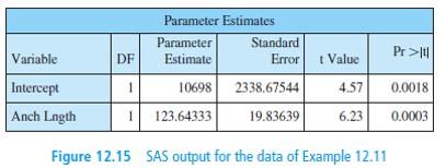
26 Example When damage to a timber structure occurs, it may be more economical to repair the damaged area rather than replace the entire structure The dependent variable is y = rupture load (N) and the independent variable is anchorage length (the additional length of material used to bond at the junction), in mm

27

28 Example Main quantities are S xx = 18, 000 error df 10 2 = 8, s = The estimated standard error is The 95% confidence interval is s Sxx = ± (2.306)(19.836) = (77.90, )

29 Hypothesis testing The most common is the model utility test H 0 : β 1 = 0 vs. H a : β 1 0 The test statistic value is t = ˆβ 1 β 10 s ˆβ1 Then, if e.g. H a : β 1 > β 10, we have the P-value as the area under the t n 2 curve to the right of t

30 Example Mopeds are very popular in Europe because of cost and ease of operation They can be dangerous if performance characteristics are modified. One of the features commonly manipulated is the maximum speed simple linear regression analysis of the variables x = test track speed (km/h) and y = rolling test speed

31

32 Regression and ANOVA Note that t 2 = f for the test of H 0 : β 1 = 0 vs. H a : β 1 0

33

34 Inference about the mean µ Y x For a given value x, the estimated average value of Y is ˆβ 0 + ˆβ 1 x It can also be viewed as the prediction at the given point x It is possible to represent the estimated average value of Y as ˆβ 0 + ˆβ 1 x = n d i Y i i=1 where d i = 1 n + (x x)(x i x) n i=1 (x i x) 2

35 Summary E(Ŷ ) = β 0 + β 1 x, and the variance is [ 1 V (Ŷ ) = σ 2 n + (x x) 2 ] The estimated variance results from the above by replacing σ 2 with s; Ŷ is also normally distributed To construct a confidence interval or to test a hypothesis, just note that T = Ŷ ( ˆβ 0 + ˆβ 1 x ) t n 2 SŶ S xx

36 Inferences concerning µ Y x The variable T = ˆβ 0 + ˆβ 1 x (β 0 + β 1 x ) S ˆβ0 + ˆβ 1 x = Ŷ (β 0 + β 1 x ) SŶ has a t distribution with n 2 df The 100%(1 α) CI for E (Y x ) = µ Y x is ˆβ 0 + ˆβ 1 x ± t α/2,n 2 s ˆβ 0 + ˆβ 1 x = ŷ ± t α/2,n 2 sŷ

37 Example Corrosion of steel reinforcing bars is the most important durability problem for reinforced concrete structures Representative data on x = carbonation depth (mm) and y = strength (MPa) for a sample of core specimens from a building in Singapore The scatter plot supports the use of simple linear regression; thus, let us obtain 95% CI for β 0 + β 1 45 for x = 45 mm

38 Example First, ˆβ 1 = and ˆβ 0 = so The estimated ŷ = = sŷ = ) Th 16 df t-critical value is and so = ± (2.120)(.7582) = (12.18, 15.40)

39 Example The following output results from a request to fit the simple linear regression model and calculate confidence intervals for the mean value of strength at depths of 45 mm and 35 mm

40

41 CI s for multiple values of x In some situations, a CI is desired not just for a single x value but for two or more x values Suppose an investigator wishes a CI both for µ Y v and for µ Y w, where v and w are two different values of the independent variable The intervals are not independent because the same ˆβ 0, ˆβ 1 and S are used in each. We therefore cannot assert that the joint confidence level for the two intervals is exactly 90% even if we select α = 0.05 It can be shown, though, that if the 100%(1 α) CI is computed both for x = v and x = w to obtain joint CIs for µ Y v and for µ Y w, then the joint confidence level on the resulting pair of intervals is at least 100%(1 2α).

42 A prediction interval for a future value of Y Sometimes, an investigator may wish to obtain an interval of plausible values for the value of Y associated with some future observation when the independent variable has value x We may want to relate vocabulary size y to the age of a child x. The CI with x = 6 would provide an estimate of true average vocabulary size for all 6-year-old children Alternatively, we might wish an interval of plausible values for the vocabulary size of a particular 6-year-old child

43 The error of prediction The error of prediction is Y ( ˆβ 0 + ˆβ 1 x ) The variance of the prediction error is [ V (Y ( ˆβ 0 + ˆβ 1 x )) = σ n + (x x) 2 ] The expected value of the prediction error is E (Y ( ˆβ 0 + ˆβ 1 x )) = 0 and S xx T = Y ( ˆβ 0 + ˆβ 1 x ) S n + (x x) 2 S xx t n 2

44 Prediction interval The prediction interval is ˆβ 0 + ˆβ 1 x ± s n + (x x) 2 S xx This interval is always wider than the corresponding confidence interval

45 Example Lets return to the carbonation depth-strength data and calculate a 95% PI for a strength value that would result from selecting a single core specimen whose carbonation depth is 45 mm The relevant quantities are ŷ = 13.79, sŷ =.7582, s = For a prediction level of 95% based on n 2 = 16 df the critical value is The prediction interval is then ± (2.8640) 2 + (.7582) 2 = (7.51, 20.07)