ACCELERATED BUNDLE LEVEL TYPE METHODS FOR LARGE SCALE CONVEX OPTIMIZATION

Transcription

1 ACCELERATED BUNDLE LEVEL TYPE METHODS FOR LARGE SCALE CONVEX OPTIMIZATION By WEI ZHANG A DISSERTATION PRESENTED TO THE GRADUATE SCHOOL OF THE UNIVERSITY OF FLORIDA IN PARTIAL FULFILLMENT OF THE REQUIREMENTS FOR THE DEGREE OF DOCTOR OF PHILOSOPHY UNIVERSITY OF FLORIDA 2017

2 c 2017 Wei Zhang

3 To my advisors and my family

4 ACKNOWLEDGMENTS I would like to express my sincere appreciation to my advisor Dr. Yunmei Chen. Without her professional guidance, invaluable advices and consistent support throughout my entire graduate study, this thesis would not have been possible. She is very knowledgeable and friendly. I really enjoy the experience learning from and working with her. I am deeply grateful to my Co-advisor, Dr. Guanghui Lan, for sharing me his great knowledge in nonlinear programming and optimization and giving me invaluable advices and help for my research. Next, I would like to thank Dr. Scott Mccullough, Dr. Michael Jury, Dr. Krishnaswami Alladi and Dr. Samuel Wu for serving as my doctoral committee members, attending my oral exam and Ph.D defense and providing constructive advices to my research and thesis. Furthermore, I would like to thank Dr. Jean Larson and Dr. Perter Sin for serving as our graduate coordinate, Dr. Scott Mccullough and Dr. Yunmei Chen for writing recommendation letters for me, I really appreciate their help and kindness. I would also like to thank all Dr. Chen s group members, Ouyang Yuyuan, Hao Zhang, Xianqi Li and Chenxi Chen for their support and discussion throughout my graduate study. Finally, and most importantly, I would express my special thanks to my family for their consistent love and support. 4

5 TABLE OF CONTENTS page ACKNOWLEDGMENTS LIST OF TABLES LIST OF FIGURES ABSTRACT CHAPTER 1 INTRODUCTION Problem of Interest Development of Bundle Level Type Methods Outline of the Dissertation FAST ACCELERATED BUNDLE LEVEL METHODS FOR CONVEX OPTIMIZATION Background Fast Accelerated Bundle Level Methods for Ball-Constrained Convex Optimization FAPL Method for Ball-Constrained Convex Optimization FUSL Method for Ball-Constrained Saddle-Point Problem Solving the Subproblem of FAPL and FUSL Methods Fast Accelerated Bundle Level Methods for Unconstrained Convex Optimization Expansion Algorithm for Unconstrained Convex Optimization Extending FAPL and FUSL for Unconstrained Convex Optimization Generalization to Strongly Convex Optimization Numerical Experiments Quadratic Programming Total Variation Based Image Reconstruction Partially Parallel Imaging ACCELERATED BUNDLE LEVEL METHODS WITH INEXACT ORACLE Background Fast Accelerated Prox-Level Methods with Inexact Oracle IFAPL Method for Smooth Ball-Constrained Convex Optimization IFAPLS Method for Unconstrained Strongly Convex Optimization Inexact Fast Uniform Smoothing Level Methods for Saddle-Point Problem IFUSL Method for Ball-Constrained Saddle-Point Problem IFUSLS Method for Strongly Convex Saddle-Point Problem ACCELERATED BUNDLE LEVEL METHODS FOR FUNCTIONAL CONSTRAINED OPTIMIZATION Background

6 4.2 ACBL Method for Functional Constrained Convex Optimization ACPL Method for Functional Constrained Convex Optimization ACSL Method for Constrained Saddle-Point Problem REFERENCES BIOGRAPHICAL SKETCH

7 Table LIST OF TABLES page 2-1 Uniformly distributed QP instances Gaussian distributed QP instances Comparison to Matlab solver Unconstrained QP instances

8 Figure LIST OF FIGURES page 2-1 TV-based reconstruction (Shepp-Logan phantom) TV-based reconstruction (brain image) Sensitivity map and Cartesian masks PPI image reconstruction (acquisition rate: 14%) PPI image reconstruction (acquisition rate: 10%)

9 Abstract of Dissertation Presented to the Graduate School of the University of Florida in Partial Fulfillment of the Requirements for the Degree of Doctor of Philosophy ACCELERATED BUNDLE LEVEL TYPE METHODS FOR LARGE SCALE CONVEX OPTIMIZATION Chair: Yunmei Chen Cochair: Guanghui Lan Major: Mathematics By Wei Zhang August 2017 This PhD dissertation is focused on developing accelerated bundle-level (BL) type methods for solving large-scale convex optimization problems (COPs) arising from many data analysis and machine learning problems. Comparing to gradient-descent type methods, the BL type methods not only achieve the optimal iteration complexities for smooth, weakly smooth and nonsmooth COPs, but also have the advantages of utilizing historical information and restricted memory to speed up convergence in practice. In the first part, we proposed several fast accelerated BL methods for ball-constrained and unconstrained COPs to improve the efficiency and applicability of the existing BL type methods. By reducing the number of involved subproblems and introducing an efficient approach to exactly solve the subproblem, the proposed methods could achieve higher accuracy of solution with faster convergence speed. The applications to quadratic programming and image processing are also presented. In the second part, we developed the inexact accelerated BL methods for solving smooth COPs and a class of saddle-point problem, where the exact first-order information of the objective function is either not available or very expensive to compute. We further extended the proposed algorithms to solve strongly convex functions with better iteration complexities, and discussed the dependence between the accuracy of the inexact oracle and the best accuracy of the approximate solution the algorithms could achieve. 9

10 In the last part, we introduced several accelerated BL methods for functional constrained optimization: min x X f(x), s.t. g(x) 0. This problem is considered to be difficult if the projection onto the feasible set {x X : g(x) 0} is hard to compute. We reduced the original problem to a non-functional constrained COP and applied the fast accelerated BL methods with some important modifications to solve the non-functional constrained COP. Moreover, by incorporating Nesterov s smoothing technique, we further extended the proposed methods to solve a class of constrained saddle-point problem. Both the iteration complexity and practical performance of the proposed algorithms are studied. 10

11 CHAPTER 1 INTRODUCTION 1.1 Problem of Interest Many data analysis problems are often modeled as the following broad class of convex optimization problem (COP): f := min f(x), (1 1) x X where X R n is a closed convex set, and f : X R is a convex function satisfying f(y) f(x) f (x), y x M 1 + ρ y x 1+ρ, x, y B( x, R), (1 2) for some M > 0 and ρ [0, 1]. We call f( ) is nonsmooth if ρ = 0, smooth if ρ = 0, and weakly smooth if 0 < ρ < 1. For example, the classic ridge regression model (namely, Tikhonov regularization) in statistical learning estimates parameters β by min y β R Aβ 2 subject to β λ, (1 3) n where denotes the Euclidean norm, y describes the observed outcome, A are the predictors in the observed data, and λ is a regularization parameter. The above model can be viewed as a special case of (1 1) with x = β, f(x) = y Ax 2, and X = {x R n : x λ}. Another important example is the classical two-dimensional total variation (TV) based image reconstruction problem given by: 1 min u R n 2 Au b 2 + λ u T V, (1 4) where A is the measurement matrix, u is the n-vector form of a two-dimensional image to the constructed, b represents the observed data, T V is the discrete TV semi-norm, and λ is the regularization parameter. Problem (1 4) can also be casted as (1 1) by setting x = u, f(x) = Ax b 2 /2 + λ x T V, and X = R n. It is worth noting that while problem (1 3) has an Euclidean ball constraint, problem (1 4) is an unconstrained COP. Moreover, the objective 11

12 function in (1 3) is smooth, while the objective function in (1 4) is defined as the summation of a smooth term Ax b 2 /2 and a nonsmooth term λ x T V. Due to the high dimensionality of x for many applications in data analysis and imaging, much recent research effort has been directed to the development of efficient first-order methods for solving (1 1). First-order methods use gradients (or subgradients) of f exclusively and hence possess significantly reduced iteration cost than second-order methods. The efficiency of these algorithms are often measured by their iteration complexity in terms of the number of (sub)gradient evaluations required to find an approximate solution of (1 1). In view of the classic complexity theory [1], for any first-order methods the number of (sub)gradient evaluations required to find an ϵ-solution of (1 1) (i.e., a point x ϵ R n satisfying f(x ϵ ) f ϵ) cannot be smaller than O(1/ϵ 2 ) if f is nonsmooth. This can be achieved, for example, by traditional subgradient methods. For a smooth f, the optimal iteration complexity is O(1/ ϵ), which can be achieved, for example, by Nesterov s accelerated gradient (AG) algorithms [2 4]. Recently, by adapting Nesterov s AG schemes and smoothing technique [2], several popular classes of first-order methods have been developed to significantly improve their iteration complexity bounds. For instance, the accelerated primal dual (APD) algorithm [5] and accelerated hybrid proximal extragradient algorithm [6], which exhibit the optimal iterative complexity for solving a broad class of saddle-point (SP) problems, and several variants of alternating direction method of multipliers (ADMM)[7 12], have improved the iteration complexity regarding to the smooth component. In this thesis, we focus on a different class of first-order methods, i.e., bundle-level (BL) type methods, which not only can achieve the optimal iteration complexities for solving smooth, weakly smooth and nonsmooth COPs but also have the advantages of utilizing restricted memory and historical first-order information through cutting plane models to significantly accelerate the numerical performance of the gradient descent type methods as mentioned above. We first give a review on several different types of BL methods. 12

13 1.2 Development of Bundle Level Type Methods The BL method originated from the well-known Kelley s cutting-plane method in 1960 [13]. Consider the COP fx := min f(x), (1 5) x X where X is a compact convex set and f is a closed convex function. The fundamental idea of the cutting plane method is to generate a sequence of piecewise linear functions to approximate f on X. In particular, given x 1, x 2,..., x k X, this method approximates f by m k (x) := max{h(x i, x), 1 i k}, (1 6) and computes the iterate x k+1 by x k+1 Argmin x X m k (x), (1 7) where h(z, x) := f(z) + f (z), x z, (1 8) and f (x) f(x), where f(x) denotes the subdifferential of f at x. Clearly, the functions m i, i = 1, 2,..., satisfy m i (x) m i+1 (x) f(x) for any x X, and are identical to f at those search points x i, i = 1,..., k. However, the inaccuracy and instability of the piecewise linear approximation m k over the whole feasible set X may affect the selection of new iterates, and the above scheme converges slowly both theoretically and practically [1, 4]. Some important improvements of Kelley s method have been made in 1990s under the name of bundle methods (see, e.g., [14 16]). In particular, by incorporating the level sets into Kelley s method, Lemaréchal, Nemirovskii and Nesterov [16] proposed in 1995 the classic BL method by performing a series of projections over the approximate level sets. Given x 1, x 2,..., x k, the classic BL iteration consists of the following three steps: a) Set f k := min{f(x i ), 1 i k} and compute a lower bound on f X by f k = min x X m k (x). 13

14 b) Set the level l k = βf k + (1 β)f k for some β (0, 1). c) Set X k := {x X : m k (x) l k } and determine the new iterate by x k+1 = argmin x Xk x x k 2. (1 9) In the BL method, the localizer X k is used to approximate the level set L k := {x : f(x) l k }, because the projection over L k is often too difficult to compute. Intuitively, as k increases, the value of l k will converge to fx, and consequently both L k and X k will converge to the set of optimal solutions to problem (3 1). It is shown in [16] that the number of BL iterations required to find an ϵ-solution to problem (3 1), i.e., a point ˆx X s.t. f(ˆx) f X ϵ, can be bounded by O(1/ϵ 2 ), which is optimal for general nonsmooth convex optimization in the black-box model. Observe that for the above BL methods, the localizer X k accumulates constraints, and hence the subproblem in Step c) becomes more and more expensive to solve. In order to overcome this difficulty, some restricted-memory BL algorithms have been developed in [15, 17]. In particular, Ben-Tal and Nemirovski [17] introduced the non-euclidean restricted memory level (NERML) method, in which the number of extra linear constraints in X k can be as small as 1 or 2, without affecting the optimal iteration complexity. Moreover, the objective function 2 in (1 9) is replaced by a general Bregman distance d( ) for exploiting the geometry of the feasible set X. NERML is often regarded as state-of-the-art for large-scale nonsmooth convex optimization as it substantially outperforms subgradient type methods in practice. Some more recent development of inexact proximal bundle methods and BL methods could be found in [18 25]. While the classic BL method was optimal for solving nonsmooth COPs only, Lan [26] recently significantly generalized this method so that it can optimally solve any black-box COPs, including nonsmooth, smooth and weakly smooth COPs. In particular, for problem (3 1) over compact feasible set X, the two new BL methods proposed in [26], i.e., the accelerated bundle-level (ABL) and accelerated prox-level (APL) methods, can solve these 14

15 problems optimally without requiring any information on problem parameters. The ABL method can be viewed as an accelerated version of the classic BL method. Same as the classic BL method, the lower bound on f X is estimated from the cutting plane model m k in (1 6), the upper bound on f X is given by the best objective value found so far. The novelty of the ABL method exists in that three different sequences, i.e., {x l k }, {x k} and {x u k }, are used for updating the lower bound, prox-center, and upper bound respectively, which leads to its accelerated iteration complexity for smooth and weakly smooth problems. The APL method is a more practical, restricted memory version of the ABL method, which also employs non-euclidean prox-functions to explore the geometry of the feasible set X. We now provide a brief description of the APL method. This method consists of multiple phases, and each phase calls a gap reduction procedure to reduce the gap between the lower and upper bounds on f by a constant factor. More specifically, at phase s, given the initial lower bound lb s and upper bound ub s, the APL gap reduction procedure sets f 0 = lb s, f 0 = ub s, l = β lb s + (1 β)ub s, and iteratively performs the following steps. a) Set x l k = (1 α k)x u k 1 + α kx k 1 and f k := max{f k 1, min{l, h k }}, where b) Update the prox-center x k by h k := where X k := {x X k 1 : h(x l k, x) l}. min h(x l x X k 1 k, x). (1 10) x k = argmin x Xk d(x), (1 11) c) Set f k = min{f k 1, f( x k )}, where x u k = α kx k + (1 α k )x u k 1, and xu k x u k or xu k 1 such that f(xu k ) = f k. is chosen as either d) Choose X k such that X k X k X k, where X k := {x X : d(x k ), x x k 0}. Here d( ) denotes the gradient of d( ). Observe that the parameters α k and β are fixed a priori, and do not depend on any problem parameters. Moreover, the localizer X k is chosen between X k and X k, so that the numbers of linear constraints in the two subproblems (1 10) and (1 11) can be fully controlled. It is shown in [26] that both the ABL and APL methods 15

16 achieve the optimal iteration complexity uniformly for smooth, weakly smooth and nonsmooth convex functions for solving problem (3 1). Moreover, by incorporating Nesterov s smoothing technique [2] into the APL method, Lan also presented in [26] that the uniform smoothing level (USL) method which can achieve the optimal complexity for solving an important class of nonsmooth structured SP problems without requiring input of any problem parameters. Because of the use of cutting plane model and the technique of restricted memory to efficiently utilize historical information, the accelerated BL methods often find a solution with much lower iteration cost and less number of iterations than many gradient decent type methods. Moreover, the BL type methods do not involve any stepsize, so do not require the input on the Lipschitz constant of the objective function. These built-in features of BL type methods are very important for solving large-scale COPs. However, the development of accelerated BL methods for various of COPs involving smooth or weakly smooth functions are still insufficient. In particular, most existing BL type methods require the feasible set to be bounded and there is no BL type methods developed for unconstrained optimization with iteration complexity proved. In many practical problems, the exact first-order information of the objective function may be unavailable or very expensive to compute, a variety of inexact BL methods [18 21, 23 25, 27 32] have been developed to deal with inexact oracle, but all these methods are non-accelerated BL methods and limited to solve nonsmooth COPs. The BL type methods also have certain advantages for solving functional constrained optimization (FCO), however, all the existing constrained BL (CBL) methods [15, 16, 33 35] can only solve nonsmooth FCO where both the objective and constraint are nonsmooth. Motivated by insufficient development and the advantages and challenges of the accelerated BL type methods, this thesis aims to develop various accelerated BL type methods to deal with general COPs, COPs with inexact oracle and FCO that have the accelerated iteration complexities for these problems and fast convergence speed in practice. 1.3 Outline of the Dissertation This thesis is organized as follows. 16

17 In Chapter 2, we propose the FAPL and the FUSL methods to improve the performance of the existing accelerated BL methods for solving smooth, weakly smooth and nonsmooth ball-constrained COPs and a class of SP problems, respectively. The FAPL and FUSL methods have significantly reduced the computational cost per iteration and increased the accuracy of the solution. Then, we introduce a general framework to extend the optimal methods for ball-constrained COPs to unconstrained COPs. The proposed framework solves unconstrained COPs through solutions to a series of ball-constrained COPs and achieves the same order of the iteration complexity as the corresponding ball-constrained COPs. The applications to large-scale least squares problems and total variation based image reconstruction problems with comparisons to related state-of-the-art algorithms are also presented. In Chapter 3, we discuss the accelerated BL type methods with inexact oracles to deal with the COPs where the exact first-order information of the objective function is either not available or too expensive to compute. Several inexact accelerated BL type methods are proposed to solve smooth COPs and a class of SP problems, with extension to strongly convex functions. Different to non-accelerated algorithms, [36] shows that the accelerated first-order methods must necessarily suffer from error accumulation of the inexact oracle. Therefore, we study the dependence between the accuracy of the inexact oracle and the best accuracy the proposed algorithms could achieve, and establish the corresponding iteration complexity bounds for converging to a solution with such accuracy guaranteed. In Chapter 4, we consider the FCO given as min x X f(x), s.t.g(x) 0. This problem is considered to be difficult if the projection onto the feasible set {x X, g(x) 0} is hard to compute. The proposed ACBL method is capable to uniformly solve FCOs with smooth, weakly smooth and nonsmooth objective and constraint, and achieves the iteration complexity O ( 1 ϵ 2/(1+3ρ) log 1 ϵ ), where ρ = min{ρf, ρ g }. Hence, if ρ f = ρ g = 0, the ACBL method achieves the same best iteration complexity as the CBL methods in [15, 16, 33] for nonsmooth FCO, and if ρ f = ρ g = 1, the ACBL method first establishes the iteration complexity ( ) O for smooth FCO. Furthermore, in order to improve the practical performance 1 ϵ log 1 ϵ 17

18 of the ACBL method, we develop the ACPL method. The ACPL method incorporates the restricted-memory technique to control the number of linear approximations used in the level set, and uses a simple strategy to update the lower estimate on f. Lastly, by employing Nesterov s smoothing technique for nonsmooth functions, we extend the ACPL method to solve a class of constrained SP problem where the objective is a SP problem and the constraint is smooth. 18

19 CHAPTER 2 FAST ACCELERATED BUNDLE LEVEL METHODS FOR CONVEX OPTIMIZATION 2.1 Background One crucial problem associated with most existing BL type methods, including APL and USL, is that each iteration of these algorithms involves solving two optimization problems: first a linear programming problem to compute the lower bound, and then a constrained quadratic programming problem to update the prox-center or new iterate. In fact, the efficiency of these algorithms relies on the solutions to these two involved subproblems, and the latter one is often more complicated than the projection subproblem in the gradient projection type methods. Moreover, most existing BL type methods require the assumption that the feasible set is bounded due to the following two reasons. Firstly, the feasible set has to be bounded to compute a meaningful lower bound by solving the aforementioned linear programming problem. Secondly, the iteration complexity analysis of those methods, such as the classical BL method [16], NERML [17], ABL, APL and USL [26], relies on the assumption that the feasible set is compact. It should be noted that there exist some variants of BL methods [18, 24, 37, 38] for solving nonsmooth COPs in which the computation of the subproblem for updating the lower bound is skipped, so that the feasible set X is allowed to be unbounded. For instance, the level bundle method in [38] updates the level parameter directly when the distance from the stability center to the newly generated iterate becomes larger than a chosen parameter. However, all these methods are limited to solve nonsmooth COPs and there is no iteration complexity analysis provided in any of these works. These issues have significantly hindered the applicability of existing BL type methods. The main purpose of this chapter is to improve the practical performance of the existing accelerated BL type methods for solving ball-constrained COPs, and further extend the BL type methods to solve unconstrained COPs with iteration complexity bounds established. In Section 2.2, we propose the FAPL and FUSL methods that greatly reduce the computational cost per iteration of the APL and USL methods for solving ball-constrained COPs. In 19

20 particular, a simple approach is introduced to exactly solve the dual problem of the only subproblem in our algorithms. In Section 2.3, we present a general framework to extend the optimal methods for ball-constrained COPs to unconstrained COPs. The proposed framework solves unconstrained COPs through solutions to a series of ball-constrained COPs and achieves the same order of iteration complexity as the corresponding ball-constrained COPs. In Section 2.4, we further extend the FAPL and FUSL method to solve strongly convex optimization problem with better iteration complexities established. In the last section, we apply the FAPL and FUSL methods to solve large-scale least squares problems and total variation based image reconstruction problems. 2.2 Fast Accelerated Bundle Level Methods for Ball-Constrained Convex Optimization In this section, we discuss the following ball-constrained COP: f x,r := min f(x), (2 1) x B(x,R) where B( x, R) := {x R n : x x R} denotes the Euclidean ball centered at x with radius R, and f : R n R is a convex function satisfying f(y) f(x) f (x), y x M 1 + ρ y x 1+ρ, x, y B( x, R), (2 2) for some M > 0 and ρ [0, 1]. This f( ) can be nonsmooth (ρ = 0), smooth (ρ = 1) and weakly smooth (0 < ρ < 1). This section contains three subsections. We first present a much simplified APL method, referred to the fast APL (FAPL) method, for solving ball-constrained black-box COPs in Subsection 2.2.1, and then present the fast USL (FUSL) method for solving a special class of ball-constrained SP problems in Subsection We show how to solve the subproblems in these two algorithms in Subsection

21 2.2.1 FAPL Method for Ball-Constrained Convex Optimization Our goal in this subsection is to present the FAPL method, which can significantly reduce the iteration cost for the APL method applied to problem (2 1). In particular, we show that only one subproblem, rather than two subproblems as in the APL method, is required in the FAPL method for defining a new iterate (or prox-center) and updating lower bound. We also demonstrate that the ball constraint in (2 1) can be eliminated from the subproblem by properly specifying the prox-function. Similarly to the APL method, the FAPL method consists of outer-inner loops, and in each outer iteration, an inner loop, the FAPL gap reduction procedure denoted by G F AP L, is called to reduce the gap between the upper and lower bounds on f x,r in (2 1) by a constant factor. We start by describing the FAPL gap reduction procedure in Procedure This procedure differs from the gap reduction procedure used in the APL method in the following several aspects. Firstly, the localizers Q k and Q k in procedure G F AP L (see Steps 1 and 4) only contain linear constraints and hence are possibly unbounded, while the localizers in the APL method must be compact. Secondly, we eliminate the subproblem that updates the lower bound on f x,r in the APL method. Instead, in the FAPL method, the lower bound is updated to the level l directly whenever Q k = or x k x > R. Thirdly, we choose a specific prox-function d(x) = 1 2 x x 2, and as a result, all the three sequences {x k }, {x l k } and {x u k } will reside in the ball B(x, R). At last, as we will show in next subsection, since the subproblem (2 6) only contains a limited number of linear constraints (depth of memory), we can solve it very efficiently, or even exactly if the depth of memory is small (e.g., less than 10). We now add a few more remarks about the technical details of Procedure Firstly, Procedure is terminated at Step 2 if Q k = or x k x > R, which can be checked automatically when solving the subproblem (2 6) (see Subsection for more details). Secondly, in Step 4, while Q k can be any polyhedral set between Q k and Q k, in practice we can simply choose Q k to be the intersection of the half-space {x R n : x k x, x x k 0} and a few most recently generated half-spaces, each of which is defined by {x R n : 21

22 The FAPL gap reduction procedure: (x +, lb + ) = G F AP L (ˆx, lb, R, x, β, θ). 0: Set k = 1, f 0 = f(ˆx), l = β lb + (1 β)f 0, Q 0 = R n, and let x u 0 = ˆx, x 0 = x. 1: Update the cutting plane model: 2: Update the prox-center and lower bound: x l k = (1 α k )x u k 1 + α k x k 1, (2 3) h(x l k, x) = f(x l k) + f (x l k), x x l k, (2 4) Q k = {x Q k 1 : h(x l k, x) l}. (2 5) x k = argmin x Qk { d(x) := 1 2 x x 2 }. (2 6) If Q k = or x k x > R, then terminate with outputs x + = x u k 1, lb+ = l. 3: Update the upper bound: set x u k = (1 α k )x u k 1 + α k x k, { (2 7) x u x u k k = k ) < f k 1, x u k 1, otherwise, (2 8) and f k = f(x u k ). If f k l + θ(f 0 l), then terminate with x + = x u k, lb+ = lb. 4: Choose any polyhedral set Q k satisfying Q k Q k Q k, where Set k = k + 1 and go to Step 1. Q k := {x R n : x k x, x x k 0}. (2 9) h(x l τ, x) l} for some 1 τ k. Finally, in order to guarantee the termination of procedure G F AP L and the optimal iteration complexity, the parameters {α k } used in this procedure need to be properly chosen. One set of conditions that {α k } should satisfy to guarantee the convergence of procedure G F AP L is given as follows: α 1 = 1, 0 < α k 1, α k c k and 1 α k+1 α 1+ρ k+1 for some constants c > 0 and ρ [0, 1]. 1 α 1+ρ k, k 1, (2 10) The following lemma provides two examples for the selection of {α k }. Lemma 1. a)if α k = 2/(k + 1), k = 1, 2,..., then the condition (2 10) is satisfied with c = 2. 22

23 b)if {α k } is recursively defined by then the condition (2 10) holds with c = 2. α 1 = 1, α 2 k+1 = (1 α k+1 )α 2 k, k 1, (2 11) Proof. Part a follows immediately by plugging α k = 2/(k + 1), k = 1, 2,..., into (2 10). For part b, it is easy to prove by induction that α k (0, 1], α k+1 < α k, k 1. Then since 1 α k+1 1 α k = α k α k+1 α k α k+1 = α k 1, k 1, α k + α k+1 2 and notice that α 1 = 1, we have 1 α k 1 k 1. Therefore α 2 k 2 < 2, k 1. Moreover, k+1 k ( ) 2 ( ) 2 ( ) 1+ρ for any k 1, 1 α k+1 = αk+1 α k by (3 16), and αk+1 α k αk+1 α k due to αk+1 < α k and ρ [0, 1]. Therefore 1 α k+1 α 1+ρ k+1 1 α 1+ρ k, k 1, hence (2 10) holds. The following lemma describes some important observations regarding the execution of procedure G F AP L. Lemma 2. Let E f (l) := {x B(x, R) : f(x) l}, the following statements hold for procedure G F AP L. a)if E f (l), then E f (l) Q k Q k Q k for any k 1. b)if Q k, then problem (2 6) in Step 2 has a unique solution. Moreover, if procedure G F AP L terminates at Step 2, then l f x,r. Proof. To prove part a, it suffices to prove that E f (l) Q k and Q k Q k for all k 1, since from the definition of Q k we already have Q k Q k Q k. we first use induction to prove the former relation. As Q 0 is set to R n, we have E f (l) Q 0. Moreover, if E f (l) Q k 1 for some k 1, then from the definition of Q k in (2 5) and the observation that h(x l k, z) f(z) l for all z E f (l), we have E f (l) Q k. To prove the relation that Q k Q k, observe that the definition of Q k in (4 71) implies that Q k = {x R n : d(x) d(x k )}. Combining such observation with the definition of x k in (2 6), we have Q k Q k and conclude part a). We now provide the proof of part b. From the definition of Q k in Step 4 and the definition of Q k in (2 5), we can see that Q k is the intersection of half-spaces, hence it is 23

24 convex and closed. Therefore, the subproblem (2 6) always has a unique solution as long as Q k is non-empty. To finish the proof it suffices to show that E f (l) = when either Q k = or x k x > R, which can be proved by contradiction. Firstly, if Q k = but E f (l), then by part a proved above, we have E f (l) Q k, which contradicts the assumption that Q k is empty. On the other hand, suppose that x k x > R and E f (l), let x R Argmin x B(x,R)f(x), it is clear that x R E f(l) Q k by a, however x R x R < x k x which contradicts the definition of x k in (2 6). Let ub := f(ˆx), ub + := f(x + ) be the input and output upper bounds on f x,r in procedure G F AP L, respectively. The following lemma shows that whenever procedure G F AP L terminates, the gap between the upper and lower bounds on f x,r is reduced by a constant factor. Lemma 3. Whenever procedure G F AP L terminates, we have ub + lb + q(ub lb), where q := max{β, 1 (1 θ)β}. (2 12) Proof. By the definition of x u k in (4 18) and the definition of f k in Step 3 of procedure G F AP L, we have f k f k 1, k 1, which implies ub + ub. Procedure G F AP L could terminate at either Step 2 or Step 3. We first assume that it terminates at Step 2 at K th iteration. The termination condition gives lb + = l = β lb + (1 β)ub, then we have ub + lb + ub β lb (1 β)ub = β(ub lb). Next suppose that Procedure terminates at Step 3 at K th iteration. We have ub + = f(x + ) = f K l + θ(ub l), since lb + lb and l = β lb + (1 β)ub, we conclude that ub + lb + l + θ (ub l) lb = [1 (1 θ)β](ub lb). The lemma is proved by combining the above two cases. We now provide a bound on the number of iterations performed by procedure G F AP L. Note that the proof of this result is similar to Theorem 3 in [26]. 24

25 Proposition 1. If the stepsizes {α k } k 1 are chosen such that (2 10) holds, then the number of iterations performed by procedure G F AP L does not exceed where := ub lb. ( ) c 1+ρ MR 1+ρ 2 1+3ρ N( ) := + 1, (2 13) (1 + ρ)θβ Proof. Suppose that procedure G F AP L does not terminate at the K th iteration for some K > 0. Then observing that x k Q k Q k 1 Q k 1 for any 2 k K due to (2 5) and (2 6), and x 1 Q 0, x 0 = argmin x Q0 d(x), we have d(x k 1 ), x k x k 1 0, 1 k K. Since d(x) is strongly convex with modulus 1, we also have d(x k ) d(x k 1 ) + d(x k 1 ), x k x k x k x k 1 2. Combining the two relations above, it implies 1 2 x k x k 1 2 d(x k ) d(x k 1 ). Summing up these inequalities for 1 k K, we conclude that 1 2 K x k x k 1 2 d(x K ) = 1 2 x K x R2. (2 14) k=1 By (2 2), (4 18), (4 19) and the convexity of f, we have for any 1 k K, f(x u k) f( x u k) h(x l k, x u k) + M 1 + ρ xu k x l k 1+ρ (2 15) = (1 α k )h(x l k, x u k 1) + α k h(x l k, x k ) + M 1 + ρ xu k x l k 1+ρ. (2 16) Since h(x l k, xu k 1 ) f(xu k 1 ), h(xl k, x k) l due to (2 5) and (2 6), and x u k xl k = α k (x k x k 1 ) due to (4 11) and (4 18), we have f(x u k) l (1 α k )(f(x u k 1) l) + α1+ρ k M 1 + ρ x k x k 1 1+ρ (2 17) 25

26 Dividing both sides of (2 17) by α 1+ρ k, and then summing up these inequalities for 1 k K, by (2 10) and the fact f(x u k ) l 0, 1 k K, we have f(x u K) l α1+ρ K M 1 + ρ Apply Hölder s inequality, and use (4 76), we have K x k x k 1 1+ρ (2 18) k=1 K k=1 x k x k 1 1+ρ K 1 ρ 2 ( K k=1 ) 1+ρ 2 x k x k 1 2 K 1 ρ 2 R 1+ρ, and a 1+ρ K c1+ρ K (1+ρ) due to (2 10). Therefore (4 44) gives f(x u K) l MR1+ρ (1 + ρ) c 1+ρ K 1+3ρ 2 (2 19) In view of Step 3 in procedure 2.2.1, and using the fact that l = β lb + (1 β)ub in Step 0, we also have f(x u K) l > θ(ub l) = θβ. Combining the above two relations, and using (2 10) and (4 76), we obtain θβ < MR1+ρ (1 + ρ) c 1+ρ K 1+3ρ 2, (2 20) which implies that ( ) c 1+ρ MR 1+ρ 2 1+3ρ K <. (2 21) (1 + ρ)θβ In view of Lemma 3 and Proposition 1, we are now ready to describe the FAPL method, which performs a sequence of calls to procedure G F AP L until an approximate solution with sufficient accuracy is found. Algorithm 1. The fast accelerated prox-level (FAPL) method 0: Given ball B(x, R), choose initial point p 0 B(x, R), tolerance ϵ > 0 and parameters β, θ (0, 1). 26

27 1: Set p 1 Argmin x B(x,R) h(p 0, x), lb 1 = h(p 0, p 1 ), ub 1 = min{f(p 0 ), f(p 1 )}, let ˆx 1 be either p 0 or p 1 such that f(ˆx 1 ) = ub 1, and s = 1. 2: If ub s lb s ϵ, terminate and output approximate solution ˆx s. 3: Set (ˆx s+1, lb s+1 ) = G F AP L (ˆx s, lb s, R, x, β, θ) and ub s+1 = f(ˆx s+1 ). 4: Set s = s + 1 and go to Step 2. For the sake of simplicity, each iteration of Procedure G F AP L is also referred to as an iteration of the FAPL method. The following theorem establishes the complexity bounds on the numbers of gap reduction procedures G F AP L and total iterations performed by the FAPL method, its proof is similar to that of Theorem 4 in [26]. Theorem 1. For any given ϵ > 0, if the stepsizes {α k } in procedure G F AP L are chosen such that (2 10) holds, then the following statements hold for the FAPL method to compute an ϵ-solution to problem (2 1). a)the number of gap reduction procedures G F AP L performed by the FAPL method does not exceed { ( )} (2R) 1+ρ M S := max 0, log 1. (2 22) q (1 + ρ)ϵ b)the total number of iterations performed by the FAPL method can be bounded by where q is defined in (3 32). N(ϵ) := S q 2 1+3ρ ( c 1+ρ MR 1+ρ (1 + ρ)θβϵ ) 2 1+3ρ, (2 23) Proof. We first prove part a). Let s := ub s lb s, without loss of generality, we assume that 1 > ϵ. In view of Step 0 in Algorithm 1 and (2 2), we have 1 f(p 1 ) h(p 0, p 1 ) = f(p 1 ) f(p 0 ) f (p 0 ), p 1 p 0 (2R)1+ρ M. (2 24) 1 + ρ Also, by Lemma 3 we can see that s+1 q s for any s 1, which implies that s+1 q s 1, s 0. 27

28 Moreover, if an ϵ-solution is found after performing S gap reduction procedures G F AP L, then we have Combining the above three inequalities, we conclude that S > ϵ S+1. (2 25) ϵ < q S 1 1 q S 1 (2R)1+ρ M, (2 26) 1 + ρ and part a) follows immediately from the above inequality. We are now ready to prove part b). In view of Lemma 3 and (2 25), we have s ϵq s S for any 1 s S. Using this estimate, part a), and Proposition 1, we conclude that the total number of iterations performed by the FAPL method is bounded by N(ϵ) = S ( c 1+ρ MR 1+ρ N s = S + (1 + ρ)θβϵ s=1 ) 2 1+3ρ S s=1 q 2(S s) 1+3ρ < S q 2 1+3ρ ( c 1+ρ MR 1+ρ (1 + ρ)θβϵ ) 2 1+3ρ, (2 27) where N s denotes the number of the iterations performed by the s th gap reduction procedure G F AP L for any 1 s S. In view of Theorem 1, the FAPL method achieves the optimal iteration complexity for solving nonsmooth, weakly smooth, and smooth COP problems, which is the same as the convergence properties of the ABL and APL methods (see [1, 4] for the discussions on the complexity theories for solving COPs, and [26] for the convergence properties of the ABL and APL methods) FUSL Method for Ball-Constrained Saddle-Point Problem In this subsection, we still consider the ball-constrained problem (2 1), but assume that its objective function is given by f(x) := ˆf(x) + F (x), (2 28) 28

29 where ˆf is a smooth convex function, i.e., L ˆf > 0 s.t. and ˆf(y) ˆf(x) ˆf(x), y x L ˆf 2 y x 2, (2 29) F (x) := max{ Ax, y ĝ(y)}. (2 30) y Y Here, Y R m is a compact convex set, ĝ := Y R is a relatively simple convex function, and A : R n R m is a linear operator. We will integrate Nesterov s smoothing technique for minimizing nonsmooth functions [2] into the FAPL method to solve problem (2 1)-(2 28) (i.e., problem (2 1) with f defined in (2 28)), which can significantly reduce the iteration cost of the USL method [26]. Let v : Y R be a prox-function with modulus σ v and denoting c v := argmin v Y v(y), by employing the idea in the important work of Nesterov [2], we can approximate F in (2 30) by the smooth function F η (x) := max{ Ax, y ĝ(y) ηv (y)}, (2 31) y Y where η > 0 is called the smoothing parameter, and V ( ) is the Bregman divergence defined by V (y) := v(y) v(c v ) v(c v ), y c v. (2 32) It was shown in [2] that the gradient of F η ( ) given by F η (x) = A y (x) is Lipschitz continuous with constant L η := A 2 /(ησ v ), (2 33) where A is the operator norm of A, A is the adjoint operator, and y (x) Y is the solution to the optimization problem (2 31). Moreover, the closeness of F η ( ) to F ( ) depends linearly on the smoothing parameter η, i.e., F η (x) F (x) F η (x) + ηd v,y, x X, (2 34) 29

30 where D v,y := max{v(y) v(z) v(z), y z }. (2 35) y,z Y Therefore, if we denote f η (x) := ˆf(x) + F η (x), (2 36) then f η (x) f(x) f η (x) + ηd v,y. (2 37) Applying an optimal gradient method to minimize the smooth function f η in (2 36), Nesterov proves in [2] that the iteration complexity for computing an ϵ-solution to problem (2 1)-(2 28) is bounded by O( 1 ϵ + 1 ). However, the values of quite a few problem parameters, such as ϵ A, σ v and D v,y, are required for the implementation of Nesterov s smoothing scheme. By incorporating Nesterov s smoothing technique [2] into the APL method, Lan developed in [26] a new bundle-level type method, namely the USL method, to solve structured problems given in the form of (2 1)-(2 28). While the USL method achieves the same optimal iteration complexity as Nesterov s smoothing scheme in [2], one advantage of the USL method over Nesterov s smoothing scheme is that the smoothing parameter η is adjusted dynamically during the execution, and an estimate of D v,y is obtained automatically, which makes the USL method problem parameter free. However, similar to the APL method, each iteration of the USL method involves the solutions to two subproblems. Based on the USL method in [26] and our analysis of the FAPL method in Section 2.2.1, we propose a fast USL (FUSL) method that solves problem (2 1)-(2 28) with the same optimal iteration complexity as the USL method, but requiring only to solve one simpler subproblem in each iteration. Similar to the FAPL method, the FUSL method has an outer-inner loops structure, and each outer iteration calls an inner loop, a gap reduction procedure denoted by G F USL, to reduce the gap between the upper and lower bounds on f x,r in (2 1)-(2 28) by a constant factor unless an ϵ-solution is found. We start by describing procedure G F USL. 30

31 The FUSL gap reduction procedure: (x +, D +, lb + ) = G F USL (ˆx, D, lb, R, x, β, θ). 0: Let k = 1, f 0 = f(ˆx), l = β lb + (1 β)f 0, Q 0 = R n, x u 0 = ˆx, x 0 = x, and η := θ(f 0 l)/(2d). (2 38) 1: Update the cutting plane model: Set x l k to (4 11), Q k to (2 5), and h(x l k, x) = h η (x l k, x) = f η (x l k) + f η(x l k), x x l k. (2 39) 2: Update the prox-center: Set x k to (2 6). If Q k = or x k x > R, then terminate with outputs x + = x u k 1, D+ = D, lb + = l. 3: Update the upper bound and the estimate of D v,y : Set x u k to (4 18), xu k to (4 19), and f k = f(x u k ). Check the following conditions: 3a) if f(x u k ) l + θ(f 0 l), then terminate with outputs x + = x u k, D+ = D, lb + = lb; 3b) if f(x u k ) > l + θ(f 0 l) and f η (x u k ) l + θ 2 (f 0 l), then terminate with outputs x + = x u k, D+ = 2D, lb + = lb. 4: Choose Q k as same as Step 4 in G F AP L. Set k = k + 1, and go to step 1. A few remarks about procedure G F USL are in place. Firstly, since the nonsmooth objective function f is replaced by its smoothed approximation f η, we replace the cutting plane model in (1 8) with the one for f η (see (3 78)). Also note that for the USL method in [26], ˆf is assumed to be a simple Lipschitz continuous convex function, and only F η is approximated by the linear estimation. However, in the FUSL method, we assume ˆf is general smooth and convex, and linearize both ˆf and F η in (3 78). Secondly, the smoothing parameter η is specified as a function of the parameter D, f 0 and l, where D is an estimator of D v,y defined by (4 96) and given as an input parameter for procedure G F USL. Thirdly, same as the FAPL method, the parameters {α k } are chosen according to (2 10). Such conditions are required to guarantee the optimal iteration complexity of the FUSL method for solving problem (2 1)-(2 28). Fourthly, similar to the FAPL method, the localizers Q k, Q k, Q k only contain a limited number of linear constraints, and there is only one subproblem (i.e., (2 6)) involved in procedure G F USL, which can be solved exactly when the depth of memory is small. The following lemma provides some important observations about procedure G F USL, which are similar to those for the USL gap reduction procedure in [26]. 31

32 Lemma 4. The following statements hold for procedure G F USL. a)if procedure G F USL terminates at Steps 2 or 3a, then we have ub + lb + q(ub lb), where q is defined by (3 32) and ub := f(ˆx), ub + := f(x + ). b)if procedure G F USL terminates at Step 3b, then D < D v,y and D + < 2D v,y. Proof. The proof of part a) is the same as that of Lemma 3, and we only prove part b) here. By the termination condition at Step 3b, we have f(x u k) f η (x u k) > θ 2 (f 0 l). We conclude from the above relation, (3 71), and (2 38) that D v,y f(xu k ) f η(x u k ) η > θ(f 0 l) 2η = D. Finally, D + < 2D v,y follows immediately from the above relation and the definition of D + in Step 3b. G F USL. The following result provides a bound on the number of iterations performed by procedure Proposition 2. Suppose that {α k } k 1 in procedure G F USL are chosen such that (2 10) holds. Then, the number of iterations performed by this procedure does not exceed L N(, D) := cr ˆf 2 A D θβ + + 1, (2 40) θβ where := f(ˆx) lb. Proof. It is easy to see that the gradient of f η in (2 28) has Lipschitz continuous gradient with constant L = L ˆf + L η, where L η and L ˆf are defined in (4 94) and (2 29), respectively. Suppose that procedure G F USL does not terminate at iteration K. As the G F USL procedure could be viewed as applying the G F AP L procedure to f η, similar to the discussion on (2 19), σ v 32

33 and notice that ρ = 1 as f η is smooth, we have f η (x u K) l c2 Ld(x K ) K 2 c2 LR 2 2K 2, (2 41) where c is defined in (2 10). Also, since procedure G F USL does not terminate at iteration K, in view of the termination condition in Step 3b and the definition of l in Step 0, we have f η (x u K) l > θβ 2. (2 42) By (2 41), (2 42), (4 94) and (2 38), we conclude that c K < 2 LR 2 θβ cr L ˆf 2 A D θβ +. (2 43) θβ σ v We are now ready to describe the FUSL method which iteratively calls procedure G F USL to solve the structured saddle point problem (2 1)-(2 28). Algorithm 2. The fast uniform smoothing level (FUSL) method 0: Given ball B(x, R), choose initial point p 0 B(x, R), prox-function v( ) for the smoothing function F η in (2 31) and (2 32), initial guess D 1 on the size D v,y in (4 96), tolerance ε > 0, and parameters β, θ (0, 1). 1: Set p 1 Argmin x B(x,R) h(p 0, x), lb 1 = h(p 0, p 1 ), ub 1 = min{f(p 0 ), f(p 1 )}, let ˆx 1 be either p 0 or p 1 such that f(ˆx 1 ) = ub 1, and s = 1. 2: If ub s lb s ϵ, terminate and output approximate solution ˆx. 3: Set (ˆx s+1, D s+1, lb s+1 ) = G F USL (ˆx s, D s, lb s, R, x, β, θ) and ub s+1 = f(ˆx). 4: Set s = s + 1 and go to Step 2. For simplicity, we say that a phase (i.e., an outer iteration) of the FUSL method occurs when s increases by 1. More specifically, similar to the USL method, we classify two types of phases in the FUSL method. A phase is called significant if the corresponding G F USL procedure terminates at Steps 2 or 3a, otherwise it is called non-significant. Clearly, if the 33

34 value of D v,y is provided, which is the assumption made in Nesterov s smoothing scheme [2], then we can set D 1 = D v,y in the schemes of both the USL and FUSL methods, and consequently, all the phases of both methods become significant. As the same as the FAPL method, an iteration of procedure G F USL is also referred to an iteration of the FUSL method. The following result establishes a bound on the total number of iterations performed by the FUSL method to find an ϵ-solution to problem (2 1)-(2 28). Note that the proof of this result is similar to that of Theorem 7 in [26]. Theorem 2. Suppose that {α k } in procedure G F USL are chosen such that (2 10) holds. Then, the total number of iterations performed by the FUSL method for computing an ϵ-solution to problem (2 1)-(2 28) is bounded by 2 N(ϵ) := S 1 + S 2 + ( where q and D v,y 2 1 q )cr A θβϵ D σ v + (S 1 + are defined by (3 32) and (4 96) respectively, and { } D v,y D := max{d 1, 2D v,y }, S 1 := max log 2, 0 D 1 and S 2 := 1 1 q )cr L ˆf θβϵ, (2 44) log 1 q 4 Dv,Y 2R A σ v ϵ Proof. We prove this result by estimating the numbers of iterations performed within non-significant and significant phases separately. Suppose that the sets of indices of the + 2R 2 L ˆf (2 45) non-significant and significant phases are {m 1, m 2,..., m s1 } and {n 1, n 2,..., n s2 } respectively. For any non-significant phase m k, 1 k s 1, we can easily see from Step 3b that. D mk+1 = 2D mk, by part b) in Lemma 4, the number of non-significant phases performed by the FUSL method is bounded by S 1 defined above, i.e., s 1 S 1. In addition, since D ms1 D, we have D mk (1/2) s 1 k D, where D is defined above. Combining the above estimates on s 1 and D mk, and in view of the fact mk > ϵ for all 1 k s 1, we can bound the number of iterations performed within the non-significant 34

35 phases by N 1 = s 1 k=1 N( mk, D mk ) s 1 k=1 N ( ϵ, D/2 ) s 1 k L ˆf S 1 cr θβϵ + 1 2cR A D S 1 + θβϵ σ v k=1 L ˆf S 1 cr θβϵ cR A ( D. 2 1)θβϵ σ v 2 (S 1 k) 2 (2 46) Applying Lemma 8 in [26] and relation (2 29), and in view of the fact that p 0, p 1 B(x, R) in Algorithm 2, the initial gap is bounded by [ 1 := ub 1 lb 1 [F (p 0 ) F (p 1 ) F (p 1 ), p 0 p 1 ] + ˆf(p0 ) ˆf(p ] 1 ) ˆf (p 1 ), p 0 p 1 4 2R A Dv,Y (2 47) σ v + 2R 2 L ˆf, (2 48) where F (p 1 ) F (p 1 ). Then for the significant phases, similar to the proof of Theorem 1, we have s 2 S 2. Moreover, for any n k, 1 k s 2, using Lemmas 3, 4, we have D nk D, nk+1 q nk, and ns2 > ϵ, which implies nk > ϵ/q s 2 k. Combine these estimates on D nk, nk and bound on s 2, we can see that the total number of iterations performed within the significant phases is bounded by N 2 = s 2 k=1 S 2 + cr S 2 + N( nk, D nk ) L ˆf θβϵ cr 1 q S 2 k=1 s 2 k=1 L ˆf θβϵ + q S 2 k 2 + N(ϵ/q s 2 k, D) S 2cR A D 2 θβϵ 2cR A θβϵ(1 q) D σ v. σ v k=1 q S 2 k (2 49) Finally, the total number of iterations performed by the FUSL method is bounded by N 1 + N 2, and thus (2 44) holds. 35

36 From (2 44) in the above theorem, we can see that the iteration complexity of the FUSL method for solving problem (2 1)-(2 28) is bounded by ( ) L ˆf O ϵ + A. (2 50) ϵ The above iteration complexity is the same as that of the Nesterov smoothing scheme in [2] and the USL method in [26]. However, both the USL and FUSL methods improve Nesterov s smoothing scheme in that both of them are problem parameter free. In addition, as detailed in Subsection below, the FUSL method further improves the USL method by significantly reducing its iteration cost and improving the accuracy for solving its subproblems Solving the Subproblem of FAPL and FUSL Methods In this subsection, we introduce an efficient method to solve the subproblems (2 6) in the FAPL and FUSL methods, which are given in the form of x c := argmin x Q 1 2 x p 2. (2 51) Here, Q is a closed polyhedral set described by m linear inequalities, i.e., Q := {x R n : A i, x b i, i = 1, 2,..., m}, where A i R n and b i R for 1 i m. Now let us examine the Lagrange dual of (2 51) given by max min 1 λ 0 x R n 2 x p 2 + m λ i [ A i, x b i ]. (2 52) It can be checked from the theorem of alternatives that problem (2 52) is solvable if and only if Q. Indeed, if Q, it is obvious that the optimal value of (2 52) is finite. On the other hand, if Q =, then there exists λ 0 such that λ T A = 0 and λ T b < 0, which implies that the optimal value of (2 52) goes to infinity. Moreover, if (2 52) is solvable and λ is one i=1 36

37 of its optimal dual solutions, then x c = p m λ i A i. (2 53) i=1 It can also be easily seen that (2 52) is equivalent to max λ λt Mλ + C T λ, (2 54) where M ij := A i, A j, C i := A i, p b i, i, j = 1, 2,..., m. Hence, we can determine the feasibility of (2 51) or compute its optimal solution by solving the relatively simple problem (2 54). Many algorithms are capable of solving the above nonnegative quadratic programming in (2 54) efficiently. Due to its low dimension (usually less than 10 in our practice), we propose a brute-force method to compute the exact solution of this problem. Consider the Lagrange dual associated with (2 54): min max L(λ, µ) := 1 λ 0 µ 0 2 λt Mλ (C T + µ)λ, where the dual variable is µ := (µ 1, µ 2,..., µ m ). Applying the KKT condition, we can see that λ 0 is a solution to problem (2 54) if and only if there exists µ 0 such that λ L(λ, µ ) = 0 and λ, µ = 0. (2 55) Note that the first identity in (2 55) is equivalent to a linear system: ( M λ 1. ) λ I m = µ 1. µ m C 1 C 2. C m, (2 56) 37

38 where I is the m m identity matrix. The above linear system has 2m variables and m equations. But for any i = 1,..., m, we have either λ i = 0 or µ i = 0, and hence we only need to consider 2 m possible cases on the non-negativity of these variables. Since m is rather small in practice, it is possible to exhaust all these 2 m cases to find the exact solution to (2 55). For each case, we first remove the m columns in the matrix (M I) which correspond to the m variables assumed to be 0, and then solve the remaining determined linear system. If all variables of the computed solution are non-negative, then solution (λ, µ ) to (2 55) is found, and the exact solution x c to (2 51) is computed by (2 53), otherwise, we continue to examine the next case. It is interesting to observe that these different cases can also be considered in parallel to take the advantages of high performance computing techniques. 2.3 Fast Accelerated Bundle Level Methods for Unconstrained Convex Optimization In this section we discuss the following unconstrained COP: f := min f(x), (2 57) x Rn where f : R n R is convex, and for any closed sets Ω R n, there exists M(Ω) > 0 and ρ(ω) [0, 1], such that f(y) f(x) f (x), y x M(Ω) 1 + ρ(ω) y x 1+ρ(Ω), x, y Ω. (2 58) The above assumption on f( ) covers unconstrained nonsmooth (ρ(ω) = 0), smooth (ρ(ω) = 1) and weakly smooth (0 < ρ(ω) < 1) COPs. We first present a generic algorithmic framework to solve unconstrained COP through solutions to a series of ball-constrained COPs in Subsection 2.3.1, then extend the FAPL and FUSL methods to unconstrained COPs with iteration complexity analysis in Subsection Expansion Algorithm for Unconstrained Convex Optimization In order to analyze the computational complexity of BL methods, it is commonly assumed that the feasible set of interest is compact (e.g., [16, 17, 26]). While the compactness 38

39 assumption is essential for performing complexity analysis, the applicability of existing BL methods on unconstrained COP may be impaired. In practice, one possible workaround for BL methods to solve (2 57) may involve an assumption on the distance from a point x to an optimal solution x, namely, x B( x, R) := {x R n : x x R} for some x and R. With such an assumption, we can solve (2 57) by considering a ball-constrained COP f x,r := min f(x). (2 59) x B(x,R) It should be noted that, while the above equivalent reformulation seems straightforward, its computational complexity relies almost exclusively on the radius R. In particular, if R is close to the distance from x to X, the optimal solution set of (2 57), i.e., R D is small enough, where x := argmin x { x x : x X } and D := x x, (2 60) then the computational complexity for computing approximate solutions to the ball-constrained COP (2 59) and the original unconstrained COP (2 57) are close, and it is definitely reasonable to solve (2 59) instead. However, if R is severely overestimated, the computational complexity for solving the ball-constrained COP (2 59) may become much higher than the optimal complexity bound that depends on D. Based on the above discussion, we can conclude that a good BL method should tackle the unconstrained COP (2 57) from two perspectives. Firstly, without any satisfiable knowledge regarding D, such BL method should still be able to solve (2 57) with optimal complexity bound that depends on D. Secondly, if there exists an approximate distance R that is close to D, a good BL method should solve the ball-constrained problem (2 59) efficiently. We will consider a generic framework that follows the former perspective in this subsection, and then extend the BL method to solve (2 57) in the next subsection. In this subsection, our goal is to design a generic algorithmic framework that follows the former perspective in the above discussion, and solve the unconstrained COP (2 57) through solutions to a series of ball-constrained COPs. It should be noted that such concept indeed 39

40 follows naturally from the two perspectives discussed above: if a BL method is computationally efficient for ball-constrained COPs of form (2 59), starting from certain R for (2 59) and enlarging it by two each time, we will eventually reach a close enough estimate of D after logarithmic amount of times. Given x R n, R > 0, ϵ > 0, let us assume that there exists a first-order algorithm, denoted by A(x, R, ϵ), which can find an ϵ-solution to (2 59). In other words, we assume that each call to A(x, R, ϵ) will compute a point z B(x, R) such that f(z) fx,r ϵ. Moreover, throughout this section, we assume that the number of (sub)gradient evaluations required by A(x, R, ϵ) for finding an ϵ-solution to (2 59) is bounded by N x,r,ϵ := C 1(x, R, f)r α 1 ϵ β 1 + C 2(x, R, f)r α 2, (2 61) ϵ β 2 where α 1 β 1 > 0 and α 2 β 2 > 0. C 1 (x, R, f) and C 2 (x, R, f) are constants that depend on f in (2 59) and nondecreasing with respect to R. For example, if f is a smooth convex function, f is Lipschitz continuous in R n with constant L, i.e., (2 58) holds with ρ(r n ) = 1 and M(R n ) = L, and we apply the APL method to (2 59), then we have only one term with α 1 = 1, β 1 = 1/2, and C 1 (x, R, f) = c L in (2 61), where c is a universal constant. Observe that the two complexity terms in (2 61) will be useful for analyzing some structured COP problems in Section It should also be noted that a more accurate estimate of C 1 (x, R, f) is cm(b(x, R)), since the Lipschitz constant L = M(R n ) throughout R n is larger than or equal to the local Lipschitz constant on B(x, R). Let A be the algorithm that can find an ϵ-solution to ball-constrained problem (2 59). By utilizing a novel guess and check procedure, we present an expansion algorithm for unconstrained convex optimizations as follows: Algorithm 3. Expansion algorithm for unconstrained COP Choose an arbitrary r 1 > 1 and compute the initial gap 1 := f(x) min x B(x,r1 ) h(x, x). For k = 1, 2,..., 40

41 Step 1. Solve x k A(x, 2r k, k ). = A(x, r k, k ), then use x k as the initial point to solve x k = Step 2. If f(x k ) f(x k ) > k, update r k 2r k and go to Step 1. Step 3. Otherwise, output x k = x k, and let k+1 = k /2 and r k+1 = r k. Note that in order to reflect the flexibility we choose r 1 as any positive constant in Algorithm 3. However, from the theoretical complexity point of view, we prefer to starting with a smaller r 1 (i.e., a lower bound on D ). In fact, given the target accuracy ϵ one can derive a theoretically viable selection of r 1 given as follows. For simplicity, assume that f has Lipschitz continuous gradient with constant L, we have f(x 0 ) f L 2 x 0 x 2. If x 0 x 2ϵ/L, then x 0 already satisfies f(x 0 ) f ϵ. Therefore, we can set r 1 = 2ϵ/L. Such an estimate requires some prior information of L. It should be noted that an overestimate on L does not hurt the complexity bound, since r 1 is updated exponentially fast and will approach D quickly. Steps 1 and 2 in Algorithm 3 constitute a loop for finding a pair of solutions (x k, x k ) satisfying 0 f(x k ) f(x k ) k for any k 1. Since x k and x k are k-optimal solutions to min x B(x,rk ) f(x) and min x B(x,2rk ) f(x) respectively, this loop must terminate in finite time, because it will terminate whenever r k D. For simplicity, we call it an expansion if we double the radius in Step 2. Each iteration may contain several expansions before outputting solution x k in Step 3. Note that, for the implementation of Algorithm 3, most computational work exists in Step 1, which involves a sequence of calls to algorithm A. However, notice that the gaps ( k ) and radiuses (r k ) for these calls are monotonically decreasing and increasing, respectively, numerous computational cost could be saved by using results from previous expansions and iterations. For instance, the output solutions of previous calls to A associated with larger gaps or smaller radiuses could always be used as the starting point for the current call to A. For successive expansions, if the previous execution of Step 1 called A( x, r k, k ) and A( x, 2r k, k ) and the current execution of Step 1 calls A( x, 2r k, k ) and A( x, 4r k, k ), the computation of call A( x, 2r k, k ) could 41

42 be saved. Moreover, if A is referred to some specific algorithms, such as BL type methods, more previous results, like the lower bounds and prox-centers, could also be utilized to save computational cost. Note that there are proximal bundle methods incorporating with trust region techniques for updating the new iterate [39, 40]. In [39] an quadratic cutting plane model based method and in [40] the idea of Chebychev center were used to generate the trust regions. These trust region methods restrict the iterates in the trust region for better convergence to the optimal solution, while the approximate solutions in the searching balls generated by our expansion algorithm are used only for checking whether or not the current searching ball needs to be expanded in order to get a better estimate of D. Before analyzing the iteration complexity of Algorithm 3, we discuss some important observations related to the aforementioned expansions. Lemma 5. Let x R n and r > 0 be a constant, x 1 and x 2 be -solutions to COPs f x,r := respectively. If 0 f(x 1 ) f(x 2 ), then we have min f(x) and fx,2r := min f(x), (2 62) x B(x,r) x B(x,2r) f(x 2 ) f where f and D are defined in (2 57) and (2 60) respectively. ) (3 + 2D, (2 63) r Proof. Clearly, by definition, we have x 1 x r, x 2 x 2r, 0 f(x 1 ) f x,r and 0 f(x 2 ) f x,2r. It suffices to consider the case when f x,2r > f and x x > 2r, since otherwise (2 63) holds trivially. Suppose x 1 and x 2 are the solutions to the first and second problems in (2 62) respectively, let ˆx be the intersection of the line segment (x, x 1) with the ball B(x, 2r), and denote R 1 := ˆx x 1 and R 2 := x x 1. Clearly, ˆx = (1 R 1 R 2 )x 1 + R 1 R 2 x. By the convexity of f( ), we have f(ˆx) (1 R 1 R 2 )f(x 1) + R 1 R 2 f(x ), (2 64) 42

43 which implies that R 1 R 2 [f(x 1) f(x )] f(x 1) f(ˆx), (2 65) and that f(ˆx) f(x 1) due to the fact that f(x ) f(x 1). Also, we have f(ˆx) f(x 2) since ˆx B(x, 2r). In addition, f(x 1) f(x 2) = [f(x 1) f(x 1 )] + [f(x 1 ) f(x 2 )] + [f(x 2 ) f(x 2)] (2 66) = 2. (2 67) Combining the previous inequalities, we obtain f(x 1) 2 f(x 2) f(ˆx) f(x 1), (2 68) which implies that f(x 1) f(ˆx) 2. Using (2 65), and the fact that R 1 r and R 2 D + r, we have f(x 1) f(x ) 2R 2 R 1 ) (2 + 2D. r Therefore, f(x 2 ) f(x ) f(x 1 ) f(x ) [f(x 1 ) f(x 1)] + [f(x 1) f(x )] ) (3 + 2D. r We are now ready to prove the iteration complexity of Algorithm 3 for solving the unconstrained COP (2 57). Theorem 3. Suppose that the number of (sub)gradient evaluations required by A(x, R, ϵ) for finding an ϵ-solution to (2 59) is bounded by (2 61). For any k 1, denote ϵ k := f(x k ) f for the output x k in Algorithm 3. Then we have a)r k r := max{r 1, 2D } for all k 1, where D is defined in (2 60); b)lim k ϵ k = 0; 43

44 c)the total number of (sub)gradient evaluations performed by Algorithm 3 for finding the ϵ k -solution x k to problem (2 57) is bounded by ( ) C 1 (x, 2 r, f) r α 1 O ϵ β 1 k + C 2(x, 2 r, f) r α 2 ϵ β 2 k. (2 69) Proof. We start by proving a), if r 1 D, then f( x k ) f( x k ) k for any k 1 and no expansion takes place, hence r k = r 1 = r. If r 1 D, from Algorithm 3, we see that expansion occurs at Step 2 if and only if f(x k ) f(x k ) > k. Hence, if r k D, this condition is not satisfied and no more expansion is performed. This implies r k < 2D. To prove b), observe that x k is used as the initial point for computing x k in Algorithm 3 and hence f( x k ) f( x k ). Combining this observation with the condition in Step 3, we have 0 f( x k ) f( x k ) k. Applying Lemma 5 implies ϵ k = f(x k) f (3 + 2D Note that the total number of expansion is bounded by S 1 := log 2 hence k decreases to 0 as k increases, we have lim k ϵ k = 0. r r 1 r k ) k. (2 70), (2 71) To prove c), assume that the number of executions of Step 1 in Algorithm 3 for finding x k is K. For any 1 j K, let A(x, R j, δ j ) and A(x, 2R j, δ j ) be called in the j th execution of Step 1. By using (2 61) and noting that C 1 (x, R, f) and C 2 (x, R, f) are nondecreasing with respect to R, we have the number of (sub)gradient evaluations performed by the j th execution of Step 1 is bounded by N j := (1 + 2α 1 )C 1 (x, 2R j, f)r α 1 j δ β 1 j + (1 + 2α 2 )C 2 (x, 2R j, f)r α 2 j. (2 72) δ β 2 j Let N j and N j be the first and second terms on the right of (2 72), respectively. The (j + 1) th execution of Step 1 either doubles the radius or reduces the gap by half comparing to the j th execution, i.e., R j+1 = 2R j or δ j+1 = δ j /2 respectively. Therefore we have either 44

45 N j+1 2 α 1 N j and N j+1 2 α 2 N j, or N j+1 2 β 1 N j and N j+1 2 β 2 N j. Since 2 α 1 2 β 1 > 1 and 2 α 2 2 β 2 > 1, we can combine these two cases and have N j 2 β 1 N j+1 and N j 2 β 2 N j+1, for 1 j K 1, (2 73) which further implies N j 2 β 1(K j) N K and N j 2 β 2(K j) N K, for 1 j K. (2 74) Then the total number of (sub)gradient evaluations performed by these K executions of Step 1 in Algorithm 3 is bounded by N : = K j=1 < N K (N j + N j ) N K + j=0 2 β 1j + N K K 2 β1(k j) + N K j=1 + j=0 (1 + 2α 1 )C 1 (x, 2r k, f) 1 2 β 1 2 β 2j rα 1 k β 1 k K j=1 2 β 2(K j) (2 75) N 1 β 1 K N β 2 K (2 76) + (1 + 2α 2 )C 2 (x, 2r k, f) 1 2 β 2 rα 2 k β 2 k. (2 77) The last inequality follows from the observation that the last (i.e., K th ) execution of Step 1 before x k is found has R K = r k and δ K = k. Combining the above inequality with (2 70), we have N < 2 i=1 (1 + 2 α i )C i (x, 2r k, f) 1 2 β i rα i k (3 + 2D r k ϵ β i k ) β i. (2 78) Since α i β i > 0, C i (x, 2r k, f)r α i 2D k (3 + r k ) β i = C i (x, 2r k, f)r α i β i k (3r k + 2D ) β i for i = 1, 2 are monotonically increasing with respect to r k, which, in view of the fact r k < 2 r proved by part a), therefore clearly implies Hence the proof is complete. N < 2 (2 3β i + 2 α i+3β i )C i (x, 2 r, f) rαi. (2 79) 2 β i 1 ϵ β i k i=1 Note that to solve the unconstrained COP (2 57), the termination criterions of most first-order algorithms are based on the residual of the (sub)gradient, which would lead to 45

46 different complexity analysis. To the best of our knowledge, without any prior information on D, there is no verifiable termination criterion based on functional optimality gap that could guarantee the termination of algorithms for finding an ϵ-solution to (2 57). Comparing to Nesterov s optimal gradient method for unconstrained problems in [3], Algorithm 3 only provides efficiency estimates about ϵ k := f(x k ) f when the output x k is updated, while the optimal gradient method could have estimates about ϵ k := f(x k ) f for each iterate x k. For both methods the efficiency estimates involve D. Since Algorithm 3 extends methods for ball-constrained COPs to solve (2 57), and the iterations in the expansions of Algorithm 3 could be regarded as a guess and check procedure to estimate D, it is reasonable that the efficiency estimates are only provided for unexpansive steps, i.e., Step 3 of Algorithm 3, which output x k. It has been shown in [26] that the APL method and its variant, the USL method, achieve the optimal iteration complexities in (2 59) for smooth, nonsmooth and weakly smooth COPs and a class of structured saddle point problems respectively, on any convex and compact feasible set. So Algorithm 3 could be incorporated to solve (2 57) with the optimal iteration complexities too. Therefore, the remaining part of this paper will focus on how to improve the efficiency of these BL type methods for solving ball-constrained COPs Extending FAPL and FUSL for Unconstrained Convex Optimization In this subsection, we study how to utilize the FAPL and FUSL methods to solve the unconstrained problems based on our results in Section 2.3. Let us first consider the case when f in (2 57) satisfies (2 58). If the method A in Step 1 of Algorithm 3 is given as the FAPL method, then by Theorem 1, and the fact that only one (sub)gradient of f is computed in each iteration of the FAPL method, the number of (sub)gradient evaluations within one call to A(x, R, ϵ) is bounded by N(ϵ) given by (2 30). Therefore, for the FAPL method, we have α 1 = 2(1+ρ) 3+2ρ, β 1 = 2 1+3ρ, C 1(x, R, f) = C M 2 1+3ρ and C 2 (x, R, f) = α 2 = β 2 = 0 in (2 61), where C is a constant depending on the parameters q, θ, β, ρ and c in the FAPL method. Letting ϵ k := f(x k ) f for k 1 in Algorithm 3 and 46

47 applying Theorem 3, we then conclude for finding the ϵ k -solution x k to problem (2 57), the total number of (sub)gradient evaluations performed by Algorithm 3 is bounded by ( [M(2r) ] 2 ) 1+ρ 1+3ρ O, (2 80) where M := M(B(x, 2r)), ρ := ρ(b(x, 2r)) and r is defined in part a) of Theorem 3. It ϵ k should be noted that the constants M and ρ are local constants that depend on the size of the initial ball, i.e., r 1, and the distance from x and x, which are not required for the FAPL method and Algorithm 3, and also generally smaller than the constants M(R n ) and ρ(r n ), respectively, for the global Hölder continuity condition. Moreover, if f in (2 57) is given in the form of (2 28) as a structured nonsmooth COP, then the FUSL method could be applied to solve the corresponding structured ball-constrained problems in Algorithm 3. By Theorem 2, the number of (sub)gradient evaluations of f within one call to A(x, R, ϵ) is bounded by L S 1 + S 2 + C ˆf R ϵ + C R A, (2 81) ϵ where C, C are some constants depending on the parameters q, θ, β, σ v, c, D 0 and D v,y in the FUSL method. Applying Theorem 3 with α 1 = α 2 = 1, β 1 = 1 2, β 2 = 1, C 1 (x, R, f) = C L ˆf, and C 2 (x, R, f) = C A, we conclude that the total number of (sub)gradient evaluations performed by Algorithm 3 to find the ϵ k -solution x k to problem (2 57)-(2 28) is bounded by L O 2C ˆf r + 2C r A. (2 82) ϵ k ϵ k Similar to the FAPL method, here L f := L f (B(x, 2r)) is a lower bound of L f (R n ). 47

48 2.4 Generalization to Strongly Convex Optimization In this section, we generalize the FAPL and FUSL methods for solving convex optimization problems in the form of (1 1) whose objective function f satisfies f(y) f(x) f (x), y x µ 2 y x 2, x, y R n, (2 83) for some µ > 0. For the sake of simplicity, we assume throughout this section that an initial lower bound lb 0 f is available 1. Under this assumption, it follows from (3 51) that p 0 x 2 2[f(p 0 ) lb 0 ]/µ for a given initial point p 0, and hence that the FAPL and FUSL methods for ball-constrained problems can be directly applied. However, since the lower and upper bounds on f are constantly improved in each phase of these algorithms, we can shrink the ball constraints by a constant factor once every phase accordingly. We show that the rate of convergence of the FAPL and FUSL methods can be significantly improved in this manner. We first present a modified FAPL method for solving black-box COPs which satisfy both (3 2) and (3 51). More specifically, we modify the ball constraints used in the FAPL method by shifting the prox-center x and shrinking the radius R in procedure G F AP L. Clearly, such a modification does not incur any extra computational cost. This algorithm is formally described as follows. The modified FAPL gap reduction procedure: (x +, lb + ) = G F AP L (ˆx, lb, r, β, θ) In FAPL gap reduction procedure, set x = ˆx, and consequently the prox-function d in (2 6) is replaced by x ˆx 2 /2. Algorithm 4. The modified FAPL method for strongly convex optimization In Algorithm 1, change steps 0, 1 and 3 to the following steps. 0: Choose initial lower bound lb 1 f, initial point p 0 R n, initial upper bound ub 1 = f(p 0 ), tolerance ϵ > 0 and parameters β, θ (0, 1). 1 Otherwise, we should incorporate a guess-and-check procedure similar to the one in Section

49 1: Set ˆx 1 = p 0, and s = 1. 3: Set (ˆx s+1, lb s+1 ) = G F AP L (ˆx s, lb s, 2(f(ˆx s ) lb s )/µ, β, θ) and ub s+1 = f(ˆx s+1 ). A few remarks on the above modified FAPL method are in place. Firstly, let x be the optimal solution of problem (1 1) and define s = ub s lb s. By the definition of ub s and lb s, we have f(ˆx s ) f(x ) s, which, in view of (3 51), then implies that ˆx s x 2 2 s µ =: r2, (2 84) and x B(ˆx s, r). Secondly, similar to procedure G F AP L, if procedure G F AP L terminates at step 2, we have E f (l) B(ˆx s, r) =. Combining this with the fact x B(ˆx s, r), we conclude that l is a valid lower bound on f. Therefore, no matter whether procedure G F AP L terminates at step 2 or step 4, the gap between upper and lower bounds on f has been reduced and s+1 q s, where the q is defined in (3 32). We establish in Theorem 4 the iteration complexity bounds of the modified FAPL method for minimizing strongly convex functions. Theorem 4. Suppose that {α k } k 1 in procedure G F AP L are chosen such that (2 10) holds. Then the total number of iterations performed by the modified FAPL method for computing an ϵ-solution of problem (1 1) is bounded by ( ) M S c θβµ + 1 and S q 1 ρ 1+3ρ ( 2 1+ρ 2 c 1+ρ M θβ(1 + ρ)µ 1+ρ 2 ϵ 1 ρ 2 ) 2 1+3ρ, respectively, for smooth strongly convex functions (i.e., ρ = 1) and nonsmooth or weakly smooth strongly convex functions (i.e., ρ [0, 1)), where q is defined in (3 32), lb 1 and ub 1 are given initial lower bound and upper bound on f, and S := log 1 q ( ub1 lb 1 ϵ ). (2 85) 49

50 Proof. Suppose that procedure G F AP L does not terminate at the k th inner iteration. It then follows from (2 19) and (2 84) that f(x u k) l Mr1+ρ 1 + ρ c1+ρ. (2 86) 2 k 1+3ρ Moreover, in view of the termination condition in Step 3 and relation (2 84), we have f(x u k ) l θ(ub s l) = θβ s and r = 2 s /µ. Combining all the above observations we conclude that k ( 2 1+ρ 2 c 1+ρ M θβ(1 + ρ)µ 1+ρ 2 1 ρ 2 s ) 2 1+3ρ. (2 87) So the number of inner iterations performed in each call to procedure G F AP L is bounded by ( 2 1+ρ 2 c 1+ρ M θβ(1 + ρ)µ 1+ρ 2 1 ρ 2 s ) 2 1+3ρ + 1. (2 88) Since the gap between the upper and lower bounds on f is reduced by a constant factor in each phase, i.e., s+1 q s, it easy to see that the total number of phases is bounded by S defined above. Using the previous two conclusions and the fact that s ϵ/q S s, we can show that the total number of iterations performed by the modified FAPL method is bounded by S + ( 2 1+ρ 2 c 1+ρ M θβ(1 + ρ)µ 1+ρ 2 ϵ 1 ρ 2 ) 2 1+3ρ S s=1 1 ρ ( S s) q 1+3ρ. (2 89) Specifically, if f is smooth (ρ = 1), then the above bound is reduced to ( ) M S c θβµ + 1. (2 90) If f is nonsmooth (ρ = 0) or weakly smooth (ρ (0, 1)), then the above bound is equivalent to S + ( 2 1+ρ 2 c 1+ρ M θβ(1 + ρ)µ 1+ρ 2 ϵ 1 ρ 2 ) 2 1+3ρ S s=1 1 ρ ( S s) q 1+3ρ S q 1 ρ 1+3ρ ( 2 1+ρ 2 c 1+ρ M θβ(1 + ρ)µ 1+ρ 2 ϵ 1 ρ 2 ) 2 1+3ρ. (2 91) 50

51 Now let us consider the SP problem given by (2 28), where the smooth component ˆf is strongly convex with modulus µ. Similar to the modified FAPL method, we present a modified FUSL method for solving this strongly convex SP problem as follows. The modified FUSL gap reduction procedure: (x +, D +, lb + ) = G F USL (ˆx, D, lb, r, β, θ) In FUSL gap reduction procedure, set x = ˆx, and consequently the prox-function d is replaced by x ˆx 2 /2. Algorithm 5. The modified FUSL method for strongly convex SP problem In Algorithm 2, change steps 0,1 and 3 to the following steps. 0: Choose initial lower bound lb 1 f, initial point p 0 R n, initial upper bound ub 1 = f(p 0 ), prox-function v( ), initial guess D 1 on the size D v,y, tolerance ϵ > 0 and parameters β, θ (0, 1). 1: Set ˆx 1 = p 0, and s = 1. 3: Set (ˆx s+1, D s+1, lb s+1 ) = G F USL (ˆx s, D s, lb s, 2(f(ˆx s ) lb s )/µ, β, θ) and ub s+1 = f(ˆx s+1 ). In the following theorem, we describe the convergence properties of the modified FUSL method for solving (1 1)-(2 28) with strongly convex smooth component ˆf. Theorem 5. Suppose that {α k } k 1 in procedure G F USL are chosen such that (2 10) holds. Then we have the following statements hold for the modified FUSL method. a)the total number of iterations performed by the modified FUSL method for computing an ϵ-solution of problem (1 1)-(2 28) is bounded by (S 1 + S) 2cL ˆf θβµ A D c θβ(1 q) σ v µϵ, (2 92) where q is defined in (2 10), S 1 and D are defined in (2 45), and S is defined in (2 85). b)in particular, if D v,y is known, and set D 1 = D v,y at Step 0, then the number of iterations performed by the modified FUSL method is reduced to N(ϵ) := S 2cL ˆf θβµ A + θβ(1 cd v,y q) σ v µϵ. (2 93) 51

52 Proof. Similarly to the discussion in Theorem 2, we classify the non-significant and significant phases and estimates the numbers of iterations performed by each type of phases. Suppose that the set of indices of the non-significant and significant phases are {m 1, m 2,..., m s1 } and {n 1, n 2,..., n s2 } respectively. Then the number of nonsignificant phases is bounded by S 1, i.e., s 1 S 1. And since 1 = ub 1 lb 1, so the number of significant phases is bounded by S defined above, i.e., s 2 S 2. 2 In view of Proposition 2, and substitute r =, we have for any phase µ Ñ(, D) := 2cL ˆf θβµ + 2 A cd + 1. (2 94) θβ σ v µ Following similar discussion in Theorem 2, we have the number of iterations performed by non-significant phases in the modified FUSL method is bounded by Ñ 1 = s 1 k=1 Ñ( mk, D mk ) s 1 k=1 2cL S 1 ˆf θβµ A c D S 1 θβ σ v µϵ k=1 2cL S 1 ˆf θβµ A + θβ(1 q) Ñ(ϵ, D/2 s 1 k ) (2 95) q S 1 k 2 (2 96) c D σ v µϵ. (2 97) And the bound on number of iterations performed by all significant phases is given by Ñ 2 = s 2 k=1 Ñ( nk, D nk ) s 2 k=1 S 2cL ˆf θβµ A c D θβ σ v µϵ S 2cL ˆf θβµ A + θβ(1 q) Ñ(ϵ/q s 2 k, D) (2 98) S k=1 q S k 2 (2 99) c D σ v µϵ. (2 100) Therefore, the total number of iterations is bounded by Ñ1 + Ñ2, and thus part a) holds. 52

53 For part b), in view of Lemma 4, we can see that if D 1 = D v,y, then D s D v,y for all s 1, and all phases of the modified FUSL method are significant. Therefore, replace D nk and D in (2 98), we can conclude part b) holds. In view of the above Theorem 5, we can see that the iteration complexity of the modified FUSL method for solving the strongly convex SP problem (2 28) is bounded by O ( A / ϵ). 2.5 Numerical Experiments In this section we apply the FAPL and FUSL methods to solve a few large-scale COPs, including the quadratic programming problems with large Lipschitz constants, synthetic and real world total variation based image reconstruction problems, then compare them with some other first-order algorithms. All the algorithms were implemented in MATLAB, Version R2011a and all experiments were performed on a desktop with an Inter Dual Core 2 Duo 3.3 GHz CPU and 8G memory Quadratic Programming The main purpose of this section is to investigate the performance of the FAPL method for solving smooth COPs especially with large Lipschitz constants and demonstrate the improvement of the FAPL method comparing to some other state-of-the-art BL type methods. And since most state-of-the-art BL type methods require compact feasible sets, we consider the following quadratic programming problem: min Ax b 2, (2 101) x 1 where A R m n and b R m. We compare the FAPL method with Nesterov s optimal method (NEST) for smooth functions [2], NERML [17], and APL [26]. We also compare the FAPL method with the built-in Matlab linear system solver in view of its good practical performance. In the APL method, the subproblems are solved by MOSEK [41], an efficient software package for linear and second-order cone programming. Two cases with different choices of initial lower bound LB in these experiments are conducted: (1). LB = 0 and (2). LB =. 53

54 In our experiments, given m and n, two types of matrix A are generated. The first type of matrix A is randomly generated with entries uniformly distributed in [0,1], while the entries of the second type are normally distributed according to N(0, 1). We then randomly choose an optimal solution x within the unit ball in R n, and generate the data b by b = Ax. We apply all these four methods aforementioned to solve (2 101) with this set of data A and b, and the accuracy of the generated solutions are measured by e k = Ax k b 2. The results are shown in Tables 2-1, 2-2 and 2-3. Table 2-1. Uniformly distributed QP instances A : n = 4000, m = 3000, L = 2.0e6, e 0 = 2.89e4 Alg LB Iter. Time Acc. Iter. Time Acc. FAPL e e e e-11 APL e e e e-9 NERML e e e e-3 NEST e e-6 A : n = 8000, m = 4000, L = 8.0e6, e 0 = 6.93e4 Alg LB Iter. Time Acc. Iter. Time Acc. FAPL e e e e-10 APL e e e e-9 NERML e e e e-5 NEST e e-6 FAPL method for large dimension matrix Matrix A:m n LB Iter. Time Acc. Iter. Time Acc e e-21 L=5.0e e e e e-21 L=1.0e e e e e-21 L=1.5e e e-16 In order to investigate the efficiency of solving unconstrained COPs using the proposed expansion algorithm (i.e., Algorithm 3), we conduct two sets of experiments to compare the 54

55 Table 2-2. Gaussian distributed QP instances A : n = 4000, m = 3000, L = 2.32e4, e 0 = 2.03e3 Alg LB Iter. Time Acc. Iter. Time Acc. FAPL e e e e-10 APL e e e e-7 NERML e e e e-2 NEST e e-4 A : n = 8000, m = 4000, L = 2.32e4, e 0 = 2.03e3 Alg LB Iter. Time Acc. Iter. Time Acc. FAPL e e e e-10 APL e e e e-10 NERML e e e e-4 NEST e e-5 FAPL method for large dimension matrix Matrix A:m n LB Iter. Time Acc. Iter. Time Acc e e-21 L=5.7e e e e e-21 L=9e e e e e-21 L=1.2e e e-16 Table 2-3. Comparison to Matlab solver Matrix A:m n Matlab A\b FAPL method Time Acc. Iter. Time Acc. Uniform e e-23 Uniform e e-23 Uniform e e-23 Uniform e e-23 Gaussian e e-23 Gaussian e e-23 Gaussian e e-23 Gaussian e e-23 55

56 performance of solving the unconstrained QP problem min x R n Ax b 2 using two different strategies: one starts with small initial feasible ball, then applies the unconstrained FAPL method (i.e., incorporating the expansion algorithm with the FAPL method as subroutine A), while the other one, under the assumption that a bound on D defined in (2 60) is known, applies the ball-constrained FAPL method directly by choosing some large ball that contains at least one optimal solution. Since the performance of both methods would be affected by the distance between the initial point x 0 and the optimal solution set, in both experiments, we set x = 0, D 1, and for any initial ball B( x, R), we choose the starting point x 0 randomly within the ball and then normalize x 0 and set x 0 = R. For both methods, the initial lower bound is set 2 to, and the parameters of the FAPL method are the same. In this first experiment, A is generated randomly with entries uniformly distributed in [0, 1]. In the second experiment, we use the worst-case QP instance for first-order methods which are generated by A. Nemirovski (see the construction scheme in [4] and [1] ). When we apply the unconstrained FAPL method, the radiuses of the initial balls are chosen as 10 5 D, 10 4 D, 10 3 D, 10 2 D and 10 1 D, respectively. While the ball-constrained FAPL method is employed, the radiuses of the balls are selected as 10 5 D, 10 4 D, 10 3 D, 10 2 D and 10D, respectively. The results are shown in Table 2-4. The advantages of the FAPL method can be observed from these experiments. Firstly, it is evident that BL type methods have much less iterations than NEST especially when the Lipschitz constant of the objective function is large. Among these three BL type methods, NERML requires much more iterations than APL and FAPL, which have optimal iteration complexity for this problem. Secondly, comparing to the existing BL type methods (APL and NERML), FAPL has much lower computational cost for each iteration. The computational cost of FAPL for each iteration is just slightly larger than that of NEST. However, the costs of each iteration of APL and NERML are 10 times larger than that of NEST. 56

57 Table 2-4. Unconstrained QP instances Uniform instance: A = rand(4000, 8000) FAPL-Unconstrained FAPL-Ball constrained Radius Iter. Time Acc. Radius Iter. Time Acc. 1e e-11 1e e-10 1e e-11 1e e-10 1e e-11 1e e-11 1e e-11 1e e-11 1e e-11 1e e-11 Worst-case instance: A = Bdata(2062, 4124) FAPL-Unconstrained FAPL-Ball constrained Radius Iter. Time Acc. Radius Iter. Time Acc. 1e e-8 1e e-1 1e e-8 1e e-3 1e e-8 1e e-5 1e e-8 1e e-6 1e e-8 1e e-8 Thirdly, consider the difference between the performance of setting the initial lower bound equal to 0 and, it is also evident that FAPL is more robust to the choice of the initial lower bound and it updates the lower bound more efficiently than the other two BL type methods. Though setting the initial lower bound equal to increases the numbers of iterations for all these three BL type methods, a close examination reveals that the difference between setting the lower bound to zero and for FAPL is not so significant as that for APL and NERML, especially for large matrix, for example, the second one in Table 2-1. Fourthly, FAPL needs less number of iterations than APL, especially when the required accuracy is high. A plausible explanation is that exactly solving the subproblems provides better updating for the prox-centers, and consequently, more accurate prox-centers improve the efficiency of algorithm significantly. The experiments show that, for APL and NERML, it is hard to improve the accuracy beyond However, FAPL can keep almost the same speed for deceasing the objective value from 10 6 to Fifthly, we can clearly see from Table 2-3 that FAPL is comparable to or significantly outperforms the built-in Matlab solver for randomly generated linear systems, even though our code is implemented in MATLAB rather than lower-level languages, such as C or FORTRAN. 57

58 We can expect that the efficiency of FAPL will be much improved by using C or FORTRAN implementation, which has been used in the MATLAB solver for linear systems. Finally, from Table 2-4 it is evident that the performance of both the unconstrained FAPL method and the ball-constrained FAPL method are affected by the distance between the starting point x 0 and the optimal solution set. And improper estimations on D would increase the computational cost significantly. Comparing the results presented in the same rows of the left and right columns in Table 2-4, one can see that when the estimations are proper (i.e., R is close to D ), the performance of both methods are comparable, and when the estimations are improper, the unconstrained FAPL method requires much less iterations and CPU time and can achieve higher accuracy than the ball-constrained FAPL method. Especially, for the worst-case instance, the advantages are much more significant. In summary, due to its low iteration cost and effective usage of the memory of first-order information, the FAPL method is a powerful tool for solving ball-constrained smooth COPs especially when the number of variables is huge and/or the value of Lipschitz constant is large. And by incorporating the proposed Expansion Algorithm, the unconstrained FAPL method is very efficient for solving unconstrained COPs especially when a proper estimation on the optimal solution set is not available Total Variation Based Image Reconstruction In this subsection, we apply the FUSL method to solve the nonsmooth total variation (TV) based image reconstruction problem: 1 min u R N 2 Au b λ u T V, (2 102) where A is a given matrix, u is the vector form of the image to be reconstructed, b represents the observed data, and T V is the discrete TV semi-norm defined by u T V := N D i u 2, (2 103) i=1 58

59 where D i u R 2 is the discrete gradient (finite differences along the coordinate directions) of the i th component of u, and N is the number of pixels in the image. Note that u T V is convex and nonsmooth. One of the approaches to solve this problem is to consider the associated dual or primal-dual formulations of (2 103) based on the dual formulation of the TV norm: u T V = max p, Du, where Y = {p = (p 1,..., p N ) R 2N : p i R 2, p i 2 1, 1 i N}. p Y Consequently, we can rewrite (2 102) as a saddle-point problem: (2 104) 1 min max u R N p Y 2 Au b λ p, Du. (2 105) Note that (2 105) is exactly the form we considered in the USL and FUSL methods if we set ĝ(y) = 0. Specifically, the prox-function v(y) on Y is simply chosen as v(y) = 1 2 y 2 in these smoothing techniques. In our experiments, we consider two types of instances depending on how the matrix A is generated. Specifically, for the first case, the entries of A are normally distributed, while for the second one, the entries are uniformly distributed. For both types of instances, first, we generate the matrix A R m n, then choose some true image x ture and convert it to a vector, and finally compute b by b = Ax true + ϵ, where ϵ is the Gaussian noise with distribution ϵ = N(0, σ). We compare the following algorithms: the accelerated primal dual (APD) method [5], Nesterov s smoothing (NEST-S) method [2, 42], and the FUSL method. For our first experiment, the matrix A is randomly generated of size 4, , 384 with entries normally distributed according to N(0, 64), the image x true is a Shepp-Logan phantom generated by MATLAB. Moreover, we set λ = 10 3 and the standard deviation σ = The values of Lipschitz constants are provided for APD and NEST-S, and the initial lower bound for FUSL is set to 0. We run 300 iterations for each algorithm, and present the objective values of problem (2 102) and the relative errors defined by x k x true 2 / x true 2 in Figure 2-1. In our second experiment, the matrix A is randomly generated with entries 59

60 uniformly distributed in [0, 1]. We use a brain image [43] as the true image x true, and set m = 20, 000, λ = 10, σ = Other setup is the same as the first experiment, and the results are shown in Figure 2-2. Figure 2-1. TV-based reconstruction (Shepp-Logan phantom) We make some observations about the results in Figures 2-1 and 2-2. For the first experiment, there is almost no difference between APD and NEST-S, but FUSL outperforms both of them after 5 seconds in terms of both objective value and relative error. The second experiment clearly demonstrates the advantage of FUSL for solving COPs with large Lipschitz constants. The Lipschitz constant of matrix A in this instance is about , much larger than the Lipschitz constant (about 5.9) in the first experiment. FUSL still converges quickly and decreases the relative error to 0.05 in less than 100 iterations, while APD and NEST-S converge very slowly and more than 1, 000 iterations are required due to the large Lipschitz constants. It seems that FUSL is not so sensitive to the Lipschitz constants as the other two 60

61 Figure 2-2. TV-based reconstruction (brain image) methods. This feature of FUSL makes it more efficient for solving large-scale COPs which often have big Lipschitz constants. In summary, for the TV-based image reconstruction problem (2 102), FUSL not only enjoys the completely parameter-free property (and hence no need to estimate the Lipschitz constant), but also demonstrates significant advantages for its speed of convergence and its solution quality in terms of relative error, especially for large-scale problems Partially Parallel Imaging In this subsection, we compare the performance of the FUSL method with several related algorithms in reconstruction of magnetic resonance (MR) images from partial parallel imaging (PPI), to further confirm the observations on advantages of the FUSL method. The detailed background and description of PPI reconstruction can be found in [43]. This image 61

62 reconstruction problem can be modeled as min u C n k MFS j u f j 2 + λ j=1 N D i u 2, where n = 2 (we consider two dimensional case), u is the N-vector form of a two-dimensional complex valued image to be reconstructed, k is the number of coils (consider them as sensors) in the magnetic resonance (MR) parallel imaging system. F C n n is a 2D discrete Fourier transform matrix, S j C n n is the sensitivity map of the j-th sensor, and M R n n is a binary mask describes the scanning pattern. Note that the percentages of nonzero elements in M describes the compression ratio of PPI scan. In our experiments, the sensitivity maps {S j } k j=1 are shown in Figure 2-3, the image x true is of size shown in Figures 2-4 and 2-5, and the measurements {f j } are generated by i=1 f j = M(F S j x true + ϵ re j / 2 + ϵ im j / 2), j = 1,..., k, (2 106) where ϵ re j, ϵ im j are the noise with entries independently distributed according to N(0, σ). We conduct two experiments on this data set with different acquisition rates, and compare the FUSL method to NEST-S method, and the accelerated linearized alternating direction of multipliers (AL-ADMM) with line-search method [12]. For both experiments, set σ = , λ = 10 5, and {f j } k j=1 are generated by (2 106). In the first experiment, we use Cartesian mask with acquisition rate 14%: acquire image in one row for every successive seven rows, while for the second one, we use Cartesian mask with acquisition rate 10%: acquire image in one row for every successive ten rows. The two masks are shown in Figure 2-3. The results of the first and second experiments are shown in Figures 2-4 and 2-5, respectively. These experiments again demonstrate the advantages of the FUSL method over these state-of-the-art techniques for PPI image reconstruction, 62

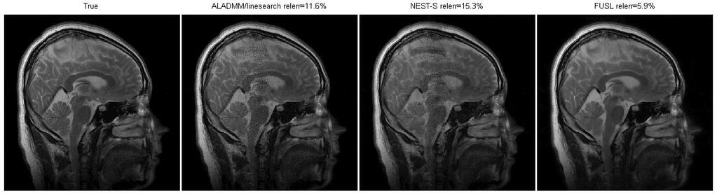
63 Figure 2-3. Sensitivity map and Cartesian masks Figure 2-4. PPI image reconstruction (acquisition rate: 14%) 63