Order Reduction of a Distributed Parameter PEM Fuel Cell Model

Transcription

1 Order Reduction of a Distributed Parameter PEM Fuel Cell Model María Sarmiento Carnevali 1 Carles Batlle Arnau 2 Maria Serra Prat 2,3 Immaculada Massana Hugas 2 (1) Intelligent Energy Limited, (2) Universitat Politècnica de Catalunya BarcelonaTech, (3) IRI (CSIC) 1 / 17 iberconappice2014

2 1 Introduction 2 Description of the system 3 Balanced truncation based model order reduction 4 Model order reduction of the PEMFC 5 Conclusions and outlook 2 / 17 iberconappice2014

3 Introduction Distributed parameter modeling required to accurately consider space variations important regarding the performance and durability of the Proton Exchange Membrane Fuel Cells (PEMFC). Large number of differential algebraic equations (DAE) obtained from discretizing a set of partial differential equations (PDE). Slow numerical simulations and difficulty to design model-based controllers. 3 / 17 iberconappice2014

4 Goal Obtaining an order reduced model, suitable to perform fast numerical simulations and design controllers for the original nonlinear model. How? Applying balanced truncation model order reduction techniques to a large dimension DAE system obtained from a first principles, PDE model of the PEMFC. Both the original full order discretized model and the reduced ones are implemented using in-house MATLAB R code. 4 / 17 iberconappice2014

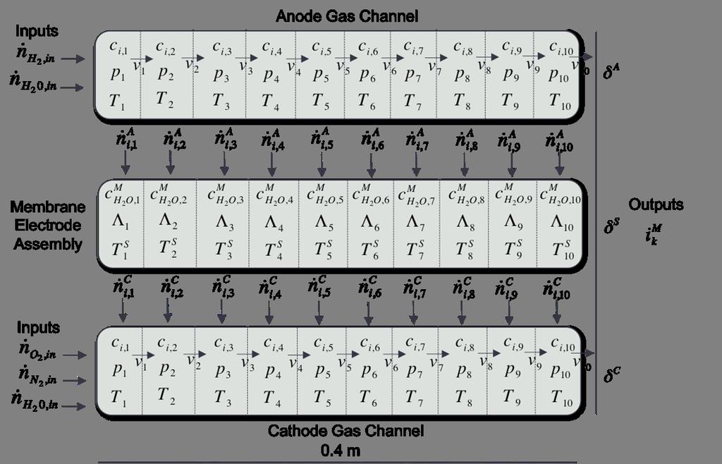
5 Description of the system Single-channel PEM Fuel Cell. 1d + 1 first principles (fluidic+thermal) simplified model for the gas channels, the gas diffusion and catalyst layers and the membrane (M. Sarmiento, M. Serra, C. Batlle, Distributed parameter model simulation tool for PEM fuel cells, International J. of Hydrogen Energy 39, (2014).) Inputs: Inlet flows of hydrogen and water (anode side), air and water (cathode side), inlet flow temperatures and cell voltage. Outputs: Membrane current profile along the channel. 10-segment grid along the channels, 110 states, 300 algebraic equations. 5 / 17 iberconappice2014

6 6 / 17 iberconappice2014

7 Balanced truncation based model order reduction Nonlinear control system (x R N, u R M, y R P, f(0) = 0) ẋ = f(x) + g(x)u, y = h(x). Controllability function L c (x) L c (x) = 1 0 inf u(t) 2 dt, x( ) = 0, x(0) = x. u L 2 ((,0),R M ) 2 Minimum 2-norm of the control to reach x from the origin. Observability function L o (x) L o (x) = y(t) 2 dt = h(x(t)) 2 dt, x(0) = x. 2-norm of the output signal obtained when the system is relaxed from the state x. 7 / 17 iberconappice2014

8 For linear control systems, ẋ = Ax + Bu, y = Cx assumed to be observable, controllable and Hurwitz, both L c (x) and L o (x) are quadratic functions L c (x) = 1 2 xt W 1 c x, L 0 (x) = 1 2 xt W o x, where W c > 0 and W o > 0, the controllability and observability Gramians, are the solutions to the matrix Lyapunov equations AW c + W c A T + BB T = 0, A T W o + W o A + C T C = 0. 8 / 17 iberconappice2014

9 W c provides information about the states that are easy to control (signals u of small norm can be used to reach them). W o allows to find the states that are easily observable (they produce outputs of large norm). One would like to select the states that score well on both counts, and this leads to the concept of balanced realization, for which W c = W o. The balanced realization is given by z = T x, and T can be computed by means of Cholesky factorizations of W c and W o. In the balanced realization, W c = W o = diag(σ 1, σ 2,..., σ N ), where σ 1 > σ 2 > > σ N > 0 are the Hankel singular values of the system. 9 / 17 iberconappice2014

10 The state with only nonzero coordinate z i is both easier to control and easier to observe than the one corresponding to z i+1. Balanced realization model order reduction is performed by keeping only the r first states in the balanced realization. This yields a system of order r with the same inputs and outputs. If G r is the transfer function of the truncated system and G that of the full one, one can show that σ r+1 G G r H 2 N i=r+1 The whole procedure depends on the controls and outputs that have been selected from the beginning. Hence, model order reduction can be tailored to discuss specific variables, by choosing them as outputs. σ i. 10 / 17 iberconappice2014

11 Model order reduction of the PEMFC System linearized around an equilibrium point, corresponding to 1.98A and 0.7V. To perform the reduction, we choose as inputs the 5 inlet flows (H 2 O, N 2 and O 2 in the cathode, and H 2 O and H 2 in the anode), their 2 temperatures and the voltage (8 in total), and the full current density profile as outputs (10). Algebraic constraints are explicitly solved, resulting in a state space of dimension / 17 iberconappice2014

12 Decay of the singular values of the linearized system. From this, one sees that there are some 10 important states from the point of view of the input/output map. Those states are, however, the transformed ones, and hence have no physical interpretation (this is a drawback of the procedure). 12 / 17 iberconappice2014

13 Simulations In order to test the reduced-model behavior, step input-output responses from the original model and reduced models of different orders were simulated and compared. Time responses of important variables to a voltage step change (from 0.7V to 0.8V ) at time 3s are shown. Figures show the comparison of three different order-reduced models with the original nonlinear full order model. The conclusion is that 11 states out of 110 are sufficient to approximate de 110-state nonlinear original model. 13 / 17 iberconappice2014

14 Membrane current density at z = / 17 iberconappice2014

15 One can select different outputs and repeat the process of model reduction. Again, 11 states are good enough to capture the input/output map. O 2 concentration at z = 10. Solid part temperature at z = / 17 iberconappice2014

16 H 2 concentration at z = 3. H 2 O anode water concentration at z = / 17 iberconappice2014

17 Conclusions and outlook Promising results have been found by applying an order reduction technique to a complex distributed parameter model of a PEM Fuel Cell. Balanced truncation model order reduction has been applied to a model obtained by spatial discretization and linearization around a working (equilibrium) point. Results have shown that reducing the order of the spatially discretized distributed parameter model from 110 states down to 11 states gives a very good approximation. An interesting next step is to study the range of operating conditions (around the equilibrium) for which the reduced model is valid. Presently, we are working towards using the reduced models to design model-based controllers. 17 / 17 iberconappice2014