TITLE: Towards the Early Detection of Breast Cancer in Young Women. CONTRACTING ORGANIZATION: Boston University Boston, Massachusetts

Transcription

1 AD AWARD NUMBER: W81XWH TITLE: Towards the Early Detection of Breast Cancer in Young Women PRINCIPAL INVESTIGATOR: Assad A. Oberai, Ph.D. CONTRACTING ORGANIZATION: Boston University Boston, Massachusetts REPORT DATE: October 2005 TYPE OF REPORT: Annual PREPARED FOR: U.S. Army Medical Research and Materiel Command Fort Detrick, Maryland DISTRIBUTION STATEMENT: Approved for Public Release; Distribution Unlimited The views, opinions and/or findings contained in this report are those of the author(s) and should not be construed as an official Department of the Army position, policy or decision unless so designated by other documentation.

2 REPORT DOCUMENTATION PAGE Form Approved OMB No Public reporting burden for this collection of information is estimated to average 1 hour per response, including the time for reviewing instructions, searching existing data sources, gathering and maintaining the data needed, and completing and reviewing this collection of information. Send comments regarding this burden estimate or any other aspect of this collection of information, including suggestions for reducing this burden to Department of Defense, Washington Headquarters Services, Directorate for Information Operations and Reports ( ), 1215 Jefferson Davis Highway, Suite 1204, Arlington, VA Respondents should be aware that notwithstanding any other provision of law, no person shall be subject to any penalty for failing to comply with a collection of information if it does not display a currently valid OMB control number. PLEASE DO NOT RETURN YOUR FORM TO THE ABOVE ADDRESS. 1. REPORT DATE (DD-MM-YYYY) 2. REPORT TYPE Annual 3. DATES COVERED (From - To) 30 Sep Sep TITLE AND SUBTITLE 5a. CONTRACT NUMBER Towards the Early Detection of Breast Cancer in Young Women 5b. GRANT NUMBER W81XWH c. PROGRAM ELEMENT NUMBER 6. AUTHOR(S) 5d. PROJECT NUMBER Assad A. Oberai, Ph.D. oberaa@rpi.edu 5e. TASK NUMBER 5f. WORK UNIT NUMBER 7. PERFORMING ORGANIZATION NAME(S) AND ADDRESS(ES) 8. PERFORMING ORGANIZATION REPORT NUMBER Boston University Boston, Massachusetts SPONSORING / MONITORING AGENCY NAME(S) AND ADDRESS(ES) 10. SPONSOR/MONITOR S ACRONYM(S) U.S. Army Medical Research and Materiel Command Fort Detrick, Maryland SPONSOR/MONITOR S REPORT NUMBER(S) 12. DISTRIBUTION / AVAILABILITY STATEMENT Approved for Public Release; Distribution Unlimited 13. SUPPLEMENTARY NOTES 14. ABSTRACT Although mammography is a valuable screening tool for breast cancer, it is less effective in younger women. Further, cancers in this age group are aggressive, and survival rates are lower. There is need for an effective screening technique to complement clinical and self breast exams. Elasticity Imaging (EI) could assume this role, as it relies on extracting information from ultrasound images which are unaffected by the denseness of the breast. The application of EI to breast cancer detection utilizes the fact that tumors are stiffer than the surrounding tissue, and may be easily discerned in an image of the spatial variation of stiffness. We believe that in order to realize the true diagnostic potential of EI, the linear-elastic model which is typically used, must be replaced by a more realistic non-linear one. Experimental data suggests that this may lead to clearer differentiation of several important tissue types. Our long term goal is to develop and test an ultrasound-based methodology for generating multiple-parameter elasticity images of breast tissue for improved diagnosis and detection of breast cancer in young women. Our aim for this grant is to obtain proof of concept results. 15. SUBJECT TERMS breast cancer detection, elasticity imaging, nonlinear elasticity, poroelasticity 16. SECURITY CLASSIFICATION OF: 17. LIMITATION OF ABSTRACT a. REPORT U b. ABSTRACT U 18. NUMBER OF PAGES c. THIS PAGE U UU 59 19a. NAME OF RESPONSIBLE PERSON USAMRMC 19b. TELEPHONE NUMBER (include area code) Standard Form 298 (Rev. 8-98) Prescribed by ANSI Std. Z39.18

3 Table of Contents Introduction Body. 4 Key Research Accomplishments. 4 Reportable Outcomes. 5 Conclusions.. 6 References 7 Appendix A 8 Appendix B 32

4 1 Introduction Although mammography is a valuable screening tool for breast cancer, it is less effective in younger women ( 40 years), usually because the higher density of their breasts can obscure tumors. While the incidence of cancer in younger women is relatively low, it is still significant: an estimated 13,000 women under 40 will be diagnosed with breast cancer this year. Further, cancers in this age group tend to be more aggressive, and survival rates are lower. In light of these observations, there is need for an effective screening technique to complement clinical and self breast exams. In addition, the lack of a specific early detection screening protocol for young women is particularly disquieting to those at elevated risk. Elasticity Imaging (EI) [1] is a technique that could potentially assume this role, as it relies on extracting information from ultrasound images which are in turn unaffected by the denseness of the breast. The application of EI to breast cancer detection (see [2] for example) utilizes the fact that breast tumors tend to be significantly stiffer than the surrounding tissue [3], and can be easily discerned in an image that represents the spatial variation of stiffness properties [4]. Measurements for EI can be made by only slightly modifying the protocol for a typical sonogram, and involve recording ultrasound images of the breast as it is deformed, and registering these images to produce a displacement field. Using this displacement field, and an assumed linear elastic model for the tissue, an inverse problem is solved to compute the spatial variation of the elastic modulus. Thus EI yields additional information about the tissue (elastic modulus) at little or no extra clinical cost. While several clinical studies are currently underway to assess the utility of EI as a screening tool, we believe that in order to realize its true diagnostic potential the assumption of linear elasticity within EI must be replaced by a more realistic non-linear model. In particular, producing images of material parameters E (the elastic modulus at zero strain) and m (the degree of non-linearity of tissue) for a non-linear model where the stress (σ) is expressed in terms of the strain (ǫ) as, σ = (E/m)(e mǫ 1), will allow for a clearer differentiation of several important tissue types. For example, it is difficult to distinguish a ductal carcinoma in-situ from a phyllodes tumor based on E alone (since the ratio is about 1.1), while it should be relatively easy to do so based on m (the ratio is about 2). The opposite holds for an infiltrating ductal carcinoma and an intraductal papilloma, where the ratio of E is about 2.1, and the ratio of m is 0.93 (values taken from [3]). By replacing the linear response in the inverse problem in EI with a more informative and accurate non-linear response we propose to generate multiple, quantitative images which provide complimentary information about the tissue, instead of a single elastic modulus image. It is well known that the microvasculature vascular density is a strong predictor of prognosis in cancerous tissue. It can be show that this quantity is directly related to the microvascular filtration coefficient, which determines the rate at which fluid is carried away in the vascular compartment and hence the rate at which the tissue relaxes to an applied load. Recently, a biomechanical model which accounts for this fluid transport mechanism and the corresponding relaxation has been proposed [5]. Using this model we now wish to verify whether the strain relaxation of tissue due to fluid transport is sufficiently large to be measured by standard elastography techniques. Our hypothesis is that if this spatiotemporal relaxation of strain can indeed be measured using elastography, then an inverse algorithm can be designed based on the biomechanical model of Netti et al., which will yield 3

5 the distribution of the microvascular filtration coefficient in the tissue. This approach may offer another exciting avenue for the application of elastography to cancer detection. 2 Body The research carried out under this grant is divided into two components. One deals with the extension of elastography to non-linear elasticity imaging and the other aims to ascertain whether elasticity imaging can be used to determine the microvascular filtration coefficient (MFC). 2.1 Nonlinear Elasticity Imaging Our long term goal is to develop and test an ultrasound-based methodology for generating multiple-parameter, high-contrast elasticity images of breast tissue for improved diagnosis and detection of breast cancer in young women. In the current grant we have obtained proof of concept results for this technique. Or results are described in detail in Appendix A. 2.2 MFC feasibility study Here our goal was to determine whether changes in the microvascular filtration coefficient in cancerous tissue produce detectible changes in strain relaxation patterns, which may be measured using standard elastography techniques. This research paves the way for using elastography to determine the spatial distribution of MFC. The results of this research are described in Appendix B. 3 Key Research Accomplishments 1. Non-linear models for breast tissue: We have demonstrated that the Veronda- Westmann model [6] has a strain energy term that yields the experimentally observed exponential stress-strain behavior observed in most breast tissue [3]. 2. Algorithms: The use of a non-linear model adds computational complexity to the inverse problem. We have developed and implemented a quasi-newton, adjoint approach to solve this problem. 3. Test problems: Using an in-house suite of computer programs, we have generated synthetic displacement data (with noise) for tissue models with known elastic parameters. We have used this data to test the performance of the inversion algorithms, and the feasibility of the overall approach. 4. Poroelastic model for tissue deformation: We have implemented the model of Netti et al. in a finite element program in order to simulate the relaxation of tissue due to vascular drainage and interstitial percolation. 4

6 5. Feasibility Study: We have determined that vascular drainage (as opposed to interstitial percolation) is the main mechanism of relaxation in most vascular tissue. Through numerical simulations we have also verified that the increased value of the microvascular filtration coefficient in cancerous tissue produces changes in strain relaxation patterns, which may be measured by standard elastography techniques. 4 Reportable Outcomes 4.1 Manuscripts 1. Nonlinear elasticity imaging I: Formulation and computational solution for compressible media, by Gokhale, N.H., Oberai, A.A., and Barbone, P.E., in preparation. 2. Nonlinear elasticity imaging II: Using enhanced strain FEM to treat nearly incompressible media, by Gokhale, N.H., Oberai, A.A., and Barbone, P.E., in preparation. 3. Nonlinear elasticity imaging III: Inversions in nearly incompressible media by higher order FEM, by Gokhale, N.H., Oberai, A.A., and Barbone, P.E., in preparation. 4. Nonlinear elasticity imaging in tissue, by Gokhale, N.H., Oberai, A.A., and Barbone, P.E., in preparation. 5. Coupling between elastic strain and interstitial fluid flow: Ramifications for poroelastic imaging, by Leiderman, R., Barbone, P.E., Oberai, A.A., and Bamber, J. C., submitted to Physics in Medicine and Biology. 4.2 Presentations 1. Towards the early detection of breast cancer in young women, DOD Era of Hope Conference, Philadelphia, June, Biomechanical Imaging: Querying Mechanical Properties of Soft Tissue, In-vivo, Seminar at the Department of Mechanical Engineering, Louisiana State University, Baton Rouge, Feb. 18, Motion and Deformation Measurement from Image Sequences, Advanced Computation Seminar Series, Center for Computational Science, BU, 18 March Inferring Biomechanical Properties from Quasistatic Deformations: An introduction to associated Inverse Problems. Paul Barbone, Invited Keynote Tutorial, Fourth International Conference on the Ultrasonic Measurement and Imaging of Tissue Elasticity, Austin TX, 16 October Nonlinear Elasticity Imaging, Nachiket Gokhale, Assad Oberai, Paul Barbone. Eighth US National Congress on Computational Mechanics, Austin TX July

7 6. Progress in Biomechanical Imaging, Mike Richards, Nachiket Gokhale, Carlos Rivas, Ricardo Leiderman, Assad Oberai, Paul Barbone. 2nd International Conference on Tumor Progression & Therapeutic Resistance September Three Dimensional Ultrasound Image Registration and Shear Elastic Modulus Reconstruction, Mike Richards, Nachiket Gokhale, Carlos Rivas, Ricardo Leiderman, Assad Oberai, Paul Barbone. Fourth International Conference on the Ultrasonic Measurement and Imaging of Tissue Elasticity, October Progress in Biomechanical Imaging. Mike Richards, Nachiket Gokhale, Carlos Rivas, Ricardo Leiderman, Assad Oberai, Paul Barbone. Fourth International Conference on the Ultrasonic Measurement and Imaging of Tissue Elasticity, October Progress in Quantitative Biomechanical Imaging. Paul Barbone, Mike Richards, Nachiket Gokhale, Carlos Rivas, Ricardo Leiderman, Assad Oberai. IMA Workshop: Imaging from Wave Propagation, Institute for Mathematics and its Application, October Nonlinear Elasticity Imaging, Nachiket Gokhale, Assad Oberai, Paul Barbone, ACES- IGERT Review Meeting, 29 September Degrees Obtained Nachiket Gokhale, PhD. in Mechanical Engineering at Boston University, Nachiket will graduate around August Personnel Supported 1. Dr. Assad Oberai (PI) 2. Dr. Ricardo Leiderman (Post-Doc) 3. Nachiket Gokhale (PhD. Student) 4.5 Funding Applied for Based on Work in this Award Title: Biomechanical Imaging, PI: P.E. Barbone, Boston University, Period: 12/01/0611/30/11, Source: National Institutes of Health Total Amount: 2,574, Conclusions Through the research supported by this award we have developed, implemented and tested (on synthetic data) an approach to determine the nonlinear elastic properties of breast tissue. The next logical step will be to test this approach in an experimental setting using tissue mimicking phantoms and then in a clinical setting. If successful in a clinical setting this 6

8 approach will substantially increase the specificity of quasi-static elastography by offering more than one parameter with which to distinguish different tissue types. In addition we have established that the reported variations in microvascular filtration coefficient (MFC), which is a strong predictor of prognosis in cancerous tissues, lead to significant changes in strain relaxation. Further, these changes in strain relaxation are large enough so that they may be detected using standard ultrasound-based elastography techniques. This motivates the development of an imaging modality based on quantifying the spatial variation of MFC which could play a significant role in cancer detection. References [1] J. Ophir, I. Cespedes, H. Ponnekanti, Y. Yazdi, and X. Li. Elastography - A Quantitative Method for Imaging the Elasticity of Biological Tissues. Ultrasonic Imaging, 13: , [2] J.C. Bamber, P.E. Barbone, N.L. Bush, D.O. Cosgrove, M.M. Doyley, F.G. Fuechsel, P.M. Meaney, N.R. Miller, T. Shiina, and F. Tranquart. Progress in Freehand Elastography of the Breast. IEICE Transactions on Information and Systems, E85D (1):5 14, [3] P. Wellman, R.H. Howe, E. Dalton, and K.A. Kern. Breast Tissue Stiffness in Compression is Correlated to Histological Diagnosis. Technical report, Harvard BioRobotics Laboratory, Division of Engineering and Applied Sciences, Harvard University, [4] P.E. Barbone and J.C. Bamber. Quantitative elasticity imaging: What can and cannot be inferred from strain images. Physics in Medicine and Biology, 47: , [5] P. A. Netti, L. T. Baxter, Y. Boucher, R. Skalak, and R. K. Jain. Macro- and Microscopic Fluid Transport in Living Tissues: Application to Solid Tumors. AIChE Journal of Bioengineering, Food, and Natural Products, 43(3): , [6] Veronda D R and Westman R A. Mechanical characterization of skin finite deformations. Journal of Biomechanics, 3(1): , January

9 Appendix A 8

10 Iterative solution of the non-linear inverse elasticity problem Nachiket H Gokhale, Paul E Barbone and Assad A Oberai Department of Aerospace and Mechanical Engineering, Boston University, Boston, MA 02215,USA Abstract. We discuss and solve an inverse problem in non-linear elasticity imaging in which we recover spatial distributions of hyperelastic material parameters from measured displacement fields. This problem has applications to elasticity imaging of soft tissue because the strain dependence of the material parameters may potentially be used to differentiate between malignant and normal tissues. We account for the geometric and material non-linearity of the tissues by assuming a known hyperelastic model for the soft tissue. We formulate the problem as a minimization problem. The cost function represents the difference between the measured and predicted displacement fields. We minimize it with respect to the spatial distribution of material properties. We solve the minimization problem by a gradient based (quasi Newton) optimization approach. We calculate the gradient efficiently using the adjoint method. We present numerical examples that demonstrate the feasibility and efficiency of the approach, and compare it to linear elastic reconstructions. 1. Introduction Elasticity Imaging (EI) is an emerging medical imaging technique in which images of the spatial distribution of the elastic modulus or stiffness of soft tissues are created. The motivation and interest for persuing this goal are numerous. For example, it is well known that pathologies affect the mechanical properties of soft tissue. This is evident in breast, prostate and other tumors presenting as hard lumps, in fibrosis which is associated with a diffuse stiffening, and atherosclerosis, which means literally, hardening of the arteries. There is also interest in being able to evaluate the normal properties of many tissues whose function is primarily mechanical, such as lungs, blood vessels, muscles, (including cardiac muscle), and cartilage. Furthermore, there is now strong evidence that phenotypical cell behaviors depend relatively strongly on the mechanical properties of their immediate environments [1]. Finally, technological applications such as automated needle insertion [2] or surgical planning and simulation would benefit from patient specific a priori or even real time mechanical characterization of soft tissues. The typical procedure followed for elasticity imaging is: To whom correspondence should be addressed (gokhalen@bu.edu) At Rensselaer Polytechnic Institute, Troy, NY, from January 2006

11 Iterative solution of the non-linear inverse elasticity problem 10 (i) Tissue Deformation and image acquisition: The soft-tissue of interest is imaged while it is deforming. The source of the deformation in general may be external (e.g. manual palpation) or internal (cardiac motion). The deformation may be quasi-static or transient. (ii) Image Processing: The displacement field is calculated from the acquired images, by using either correlation based algorithms, or minimization of a suitable objective function [3]. (iii) Inverse Problem Solution: The spatial distribution of the material properties is calculated from the known (i.e. measured) displacement field. An appropriate mathematical model for the tissue deformation is selected depending upon the spatio-temperal scales of the applied deformation and the imaging system. Given the forward mathematical model and measured deformations, an inverse problem thus follows. In this paper, an efficient formulation based on the adjoint formulation is used to solve this inverse problem. Thus, elasticity imaging involves the solution of the following inverse problem: Given the displacement field in an elastic body, calculate the spatial distribution of material properties (stiffness). Most approaches used in the literature to image the stiffness [4 10] assume that the tissue can be modeled as a linear incompressible isotropic elastic solid. The goal then is to recover the shear elastic modulus distribution of the soft tissue. The linear elastic model, of course, can accurately predict small strain deformations. There are two expected practical advantages, however, to using large strains in elasticity imaging. One is that the signal-to-noise ratio of the measured deformations tends to increase with deformation magnitude. In this case, even if the stress-strain response of the tissue remains linear over the range of strains measured, the error due to geometric nonlinearity (by this, we mean the neglect of the nonlinear terms in the exact definition of strain [11] can become significant. The second advantage is the potential to measure the nonlinear behavior of the tissue itself. This behavior is itself relevant to the physiological functioning of several tissues (e.g. arterial walls, cartilage), and may be useful in distinguishing potentially cancerous lesions. It is the latter application that directly motivates our development. The evidence in [12, 13], for example, indicates that the degree of non-linearity in the stress-strain relationship of soft tissue may be an indicator of the underlying histology. In [12], the mechanical properties of soft tissue samples of the breast collected from patients during surgery were studied using indentation tests at various strain levels. The authors estimated the elastic moduli at various strain levels and found that the cancerous and benign breast tissues have significant differences in the rate of increase of stiffness with strain. The authors of [13] tested the mechanical properties of both breast and prostate tissues at three different strain rates and strain levels. They also found that cancerous tissues are much stiffer at a higher strain level as compared to fat or normal glandular tissue. Both [12, 13] make their measurements at times scales associated with quasi-static elasticity imaging ( 0.1 Hz 10 Hz), and report negligible

12 Iterative solution of the non-linear inverse elasticity problem 11 viscoelastic effects. That is, the observed elastic modulus is independent of loading frequency. Of these various applications, our primary motivating application is breast imaging, with the aim of ultimately improving detection and differential diagnosis of breast cancer. Relatively few attempts have been made to account for non-linear elastic properties of soft tissue in material property reconstruction [14 18]. Apart from the exception of [14] only constant hyperelastic parameters are recovered. In [14] the authors model soft tissue as a linear incompressible elastic material accounting only for geometric non-linearities. The relation between the stress and strain is linear. The authors develop an inversion equation for the shear modulus in an integral form and solve it to recover shear modulus distributions. The displacement fields and strain components are calculated from ultrasound images of a gel based phantom. Accuarate results were obtained for recovered shear modulus distributions of these phantoms. In [15] the authors simulated the deformation of an agar gelatin phantom using a commercial finite element code and created synthetic RF images of the deformation of the phantom. Using displacement data calcualted from these images, the relative strain ratio images were created. Nonlinear effects were observed. That is, at low strain rates, strain contrast was observed between gelatin (stiffer) and agar (softer). With increased deformation, the agar stiffened, and became roughly equal to the stiffness of gelatin. This caused a decrease in the relative strain ratio. With further increase in the load, greater differentiation is seen between the agar and gelatin. These results point to the fact that non-linear properties can indeed be used to increase differentiation in soft tissues. Similar studies were carried out by the authors in [17]. In [16] the authors develop a reconstruction procedure to calculate constant parameters (or their combinations) in hyperelastic material modls from measured force displacement curves. The study is performed both for phantoms and simulations. A similar approach to determine the hyperelastic parameters of breast tissue samples was developed in [19] and in [18] for fitting hyperelastic models with constant material parameters to Treolar and Treolar and Jones experiments on natural rubber. The method presented below was developed and motivated by applications in breast imaging, with the aim of ultimately improving detection and differential diagnosis of breast cancer [20]. In these applications the tissue is deformed quasi-statically while it is being imaged with ultrasound. Image processing yields an estimate of the deformation pointwise with the tissue, at several instants of time. The time scales of the applied deformations justify the incompessibility assumption and neglect of inertial and viscous effects [12, 13]. The deformation is typically measured in loading only, and so the quasi-elastic [21] model is justified. We therefore assume a hyperelastic model of tissue deformation. The aim is to recover, given the deformation field everywhere in the solid, the spatial distribution (in the material or reference configuration) of the tissue parameters that describe the assumed hyperelastic model.

13 Iterative solution of the non-linear inverse elasticity problem Organization of this paper This paper is organized as follows. We first describe the strong form of the forward hyperelastic problem in section 2. This serves to introduce our modeling assumptions, definitions, and field equations. We then present the weak form which leads us to the discretization and computational solution of the forward problem. The formulation of the inverse problem follows in section 3. We formulate this as a nonlinear optimization problem. Essential to its practical solution is the efficient evaluation of the gradient. We use the adjoint method and a smart iteration-initialization strategy to accomplish this, as described in section 4. We demonstrate the method on several examples in section 5. Among the several details discussed are the choice of hyperelastic model, the choice of the regularization functional, the selection of the regularization constant, the effect of the magnitude of the applied deformation on the ability to recover the nonlinear parameters, and the limits and appropriate interpretation of linear elastic reconstructions in hyperelastic contexts. 2. The Forward problem 2.1. Strong form In this section we describe the strong form of the equations of equilibrium for a hyperelastic solid undergoing finite deformations. In this manuscript, this problem is referred to as the forward problem of hyperelasticity or simply as the forward problem. Given appropriate boundary data and the distribution of material parameters inside the body, these equations may be solved to determine the deformation field φ(x) that maps every point X in the reference or material configuration to a point x in the current or spatial configuration. That is x = φ(x). The displacement field is given by U(X) = φ(x) U(X). This is illustrated in figure (1) For a complete treatment of φ(x) X x Ω 0 Ω OCUR Figure 1. The deformation diagram this problem the reader is referred to [22,23]. The assumption of hyperelasticity implies that there exists an underlying strain energy

14 Iterative solution of the non-linear inverse elasticity problem 13 density φ such that S = φ(i 1, I 2, I 3 ;β) (1) E In equation (1), E is the Green-Lagrange strain tensor and S is the second Piola- Kirchhoff stress tensor. The Green-Lagrange strain tensor may be expressed as E = 1(F T F 1), where F = X φ(x), is the gradient of the deformation φ with 2 respect to the material co-ordinates. For an isotropic solid, the strain energy density φ can depend on the deformation gradient F only through the list of invariants (denoted by I 1, I 2 and I 3 ) of the right Cauchy-Green strain tensor C = F T F. In addition it is allowed to depend on a vector of material parameters β(x), whose values may vary spatially. In relation to soft tissue mechanics, different types of tissue behavior in response to applied load or deformation may be obtained by selecting different functional forms of the strain energy function φ. The equations of equilibrium written in the reference configuration Ω 0, in the absence of body forces are: X (FS) = 0 in Ω 0 (2) U = G on Γ g (3) FS N = H on Γ h (4) In equations (2-4), Γ g and Γ h are subsets of the boundary Γ on which displacement and traction boundary data, G and H respectively, are specified. Note that, Γ = Γ h Γg and Γ h Γg =, that is, either displacement or traction boundary conditions must be specified on the entire boundary. In equation (4), N denotes a unit normal vector in the reference configuration. With this background about the strong form of the equilibrium equations, we proceed to the weak form of the hyperelasticity equations and their computational solution The weak form and its numerical solution We begin by defining functions spaces S and V, for admissible solutions and weighting functions. S = {U U i H 1 (Ω 0 ); U i = G i on Γ g } (5) V = {V V i H 1 (Ω 0 ); V i = 0 on Γ g } (6) The weak formulation of the equilibrium equations (2-4) can be obtained by multiplying equation (2) by a weighting function W V and integrating by parts. Alternatively it may be obtained directly by minimizing the total potential energy of the system. In the reference configuration it is given by: Find a displacement U S such that A(W,U;β) W i H i dω 0 = 0 W V, (7) Γ h

15 Iterative solution of the non-linear inverse elasticity problem 14 where the semi-linear form A(, ;β) is given by A(W,U;β) = W i,i F ij S JI dω 0. (8) Ω 0 The weak form may be approximated using Galerkin s method in conjunction with standard finite element basis functions to obtain an approximate numerical solution of the forward problem. This solution requires the linearization of the semilinear form A, about an arbitrary displacement field state U which yields a bilinear form A U (, ;β,u) given by A U (W, U;β,U) = d + ǫ U;β) dǫ 0A(W,U = W i,j (δ ik S JL + F ii F kk C IJKL ) U k,l dω 0. (9) Ω 0 In equation (9) C IJKL are the components of a fourth order tensor defined as follows: C = S E or C IJKL = S IJ E KL or C IJKL = 2 φ E IJ E KL (10) Since the order of differentiation does not matter, it is clear from the equation above that the fourth order tensor C possesses major symmetry, that is C IJKL = C KLIJ. Using this and the symmetry of the stress tensor S it may be verified from (9) that A U (, ;β,u) is symmetric Numerical solution The solution of the equations of equilibrium for a solid undergoing finite deformations is significantly harder than the corresponding linear, infinitesimal deformation case. The former leads to a set of nonlinear algebraic equations which may not converge for large applied loads. To overcome this problem, an incremental loading strategy is often adopted which involves applying the prescribed boundary conditions in several (n load ) load steps and using n newton Newton iterations at each step. This leads to n load n newton stiffness matrix assemblies and solves as compared to just one for the linear case. For our applications, we have found that n load 80 and n newton 6, which makes the solution of the forward problem very expensive. Further, since the formulation of the inverse hyperelasticity problem we propose in this manuscript requires a series of forward solves, it is imperative that the time taken to solve the hyperelasticity forward problem be kept within a manageable limit. In Section (4.2), we describe an approach which accomplishes this. 3. The formulation of the inverse problem We formulate the inverse problem as a constrained minimization problem and solve it using a quasi-newton optimization algorithm. Such an algorithm requires at every iteration the gradient of the objective function with respect to the optimization parameters. The gradient of the objective function is evaluated efficiently using the

16 Iterative solution of the non-linear inverse elasticity problem 15 adjoint of the linearized hyperelasticity equations. Similar approaches for solving inverse problems have been used in [4, 24 26]. We consider a generic hyperelastic material model, which depends on N β material parameters β = [β 1,,β Nβ ] T. We seek the spatial distribution of material parameters which minimizes the difference between a set of n measured displacement field U m,1,,u m,n and the corresponding set of predicted displacement fields U 1,,U n. The predicted displacement fields are constrained to satisfy the equations of equilibrium. The objective function is the square of the L 2 norm of the difference between the measured and predicted displacement fields. We have chosen the L 2 norm as it avoids the need to differentiate a noisy measured displacement field and yields a maximum likelihood estimate of the material parameters if the noise in the measured displacement fields is Gaussian [27, pp ]. The statement of the inverse problem is : Find the spatial distribution of the material parameters β such that the objective function π (defined in equation (11)) is minimized to the subject to the constraint that each deformation field satisfy the equilibrium equations, that is (1-4) or (7) and (1). The objective function π is given by π = 1 2 n w p T(U p ) T(U m,p )) N β α j β j 2 b (11) 2 p=1 In the above equation, for the p th measurement, U m,p is the measured displacement field, U p is the corresponding predicted displacement field, T is a tensor which selects the appropriate displacement components and w p represents a weighting factor. In addition, for each material property field β j, α j is a regularization parameter and b is the regularization norm. The significance of these quantities is discussed below. Remarks (i) The weighting factors w p are chosen so that all measurements contribute equally to the objective function π. This ensures that there is no bias towards measurements with large deformation. For example, if two measurements were available and one of these, say the second contained much larger displacements. Then the objective function will be more sensitive to the second field, and the minimization algorithm would be biased in favor of minimizing this field. In order to remove this bias, it may be useful to select the weights to be inversely proportional to a measure of magnitude of the displacement fields. That is w 1 = ( q 2 q 1 ) 2 and w 2 = 1 (12) where q 1,q 2 represent the magnitude of the measured displacements. (ii) Often only one component of any measured displacement vector U m,p is reliably known. This is typically the case when the imaging system has better resolution in one direction than the other. For example, when ultrasound is used to measure the deformation, reliable estimates of the displacement field are obtained in a j=1

17 Iterative solution of the non-linear inverse elasticity problem 16 direction parallel to the axis of the transducer. In such cases it might be useful to compare only the axial component of the measured displacement with the predicted displacement. In our formulation, this is accomplished by the tensor T. Assuming the axial component is along the unit vector e 2, an appropriate choice for T is T = e 2 e 2. (13) (iii) In equation (11) α j is a regularization factor, which controls the trade off between matching the predicted and measured displacement fields and certain desirable physical characteristics of the spatial distributions of the material parameters (such as smoothness). These characteristics are selected by the choice of the regularization norm 2 b. The choice of L2 norm, defined by (14) ensures that the material parameter distribution does not attain unphysically large values. The H 1 semi-norm defined in equation (15) penalizes oscillations in the solution, ensuring smoothness in the recovered material parameter distributions. The total variation diminishing (TVD) regularization norm, defined in equation (16), does just that, but does not penalize jumps in the solution. In this norm, c is a small parameter which ensures differentiability of the norm at β i = 0. In this manuscript we have chosen c = 0.1. β j 2 2 = β j 2 H1 semi = β j 2 TV D = βj 2 dω 0 (14) Ω 0 β j 2 dω 0 (15) Ω 0 β j 2 + c 2 dω 0 (16) Ω 0 4. Inverse problem solution using the adjoint method 4.1. Definition We denote the variation in a function f(x) in the direction δx by δf and it is given by: δf = D x f δx = d f(x + ǫδx) (17) dǫ ǫ 0 Here D x f is the directional derivative of the function f(x) Gradient calculation via the adjoint method In the previous section, we have formulated the inverse hyperelasticity problem as a constrained minimization problem. To solve this problem we rely on a quasi-newton algorithm which requires the gradient vector at each iteration. The computation of the gradient is by far the most expensive part of our solution algorithm. In this section we present a method to evaluate the gradient efficiently. We use the following notation: A superscript index denotes a quantity associated with the measurement indicated by the superscript. For example, U m,p I denotes the I th

18 Iterative solution of the non-linear inverse elasticity problem 17 1: Guess a homogeneous distribution for each of the material parameters β 1 (X),β 2 (X),,β Nβ (X) 2: repeat 3: Solve forward hyperelasticity problems corresponding to the current distribution of the material parameters using the previous displacement field if available 4: Solve corresponding linear adjoint problems 5: Evaluate the objective function and its gradient 6: Use a quasi-newton optimization algorithm to update the guess of the material parameters 7: until Either the objective function π is low enough or the maximum number of iterations have been reached. Figure 2. Solution of the hyperelasticity inverse problem component of the measured displacement field corresponding to the p th measurement and U p I denotes the Ith component of the predicted displacement field corresponding to the same measurement. We note that in the objective function π, (11), each U i depends on β through the equilibrium equations (1) and (7). We account for this constraint using Lagrange multipliers. We begin by writing the Lagrangian L corresponding to the objective function π and the hyperelasticity constraints. L(W,U,β) def = n w p (T(U p ) T(U m,p )) N β α j β j 2 b 2 p=1 n i=p j=1 (A(W p,u p ;β) (W p,h p ) Γ p h ) (18) In equation (18), W p is interpreted as a Lagrange multiplier enforcing the constraint of hyperelasticity for the p th predicted displacement field. In the following development we will use to the Lagrangian to derive an expression for the derivative of the objective function with respect to optimization parameters. The variations in the Lagrangian are denoted by δl and are given by n n δl = D W p L δw p + D U p L δu p + D β L δβ (19) p=1 p=1 We set the variations in L with respect to the Lagrange multipliers W p, to zero. This yields the following equation for each U p S p, A(δW p,u p ;β) (δw p,h p ) set = 0 δw p V p. (20) Note that the equation above is identical to (7) up to the superscript p. That is, each U p is required to satisfy the forward problem for that particular deformation field. Equation (20) is often referred to as the primal problem. When all U p are selected such that equation (20) is satisfied, that is when all the predicted displacement fields U p satisfy the forward elasticity equations, from (1) and (18) we have, π = L. (21)

19 Iterative solution of the non-linear inverse elasticity problem 18 Therefore on surfaces satisfying (20) we have δπ = δl. We return to (19) and set variations in L with respect to every U p equal to zero. That is, we choose values for the Lagrange multipliers W p V p such that (22) D U p L δu p set = 0, δu p V p. (23) Using (18) and (8), this equation yields A U (W p,δu p ;β,u p )+ (T(U p U m,p )) T(δU p )dω 0 Ω 0 set = 0 δu p V p (24) where the bilinear form A U (, ;β,u p ) is given by (9). Equation (24) which is used to determine W p is the adjoint of the linearized elasticity equations. Since the linearized operator is self-adjoint (see Section 2.2), this equation may be written as: Find W p V p such that A U (δu p,w p ;β,u p )+ (T(U p U m,p )) δu p set dω 0 = 0 δu p V p (25) Ω 0 Note that when U p and W p are chosen according to (20) and (25) respectively, the relation (22) holds and the first two terms in (19) vanish. As a result we have δπ = D β L δβ = n p=1 Ω 0 W p i,i F p i,j (D β S pij δβ ) dω 0 + N β α j (β j,δβ j ) b (26) Equation (26) represents the change in π due to an infinitesimal change in the material parameters in the direction of δβ. To derive an expression for the gradient for the finite dimensional problem, we expand the material parameters in terms of a basis, N β j = M A (X)b ja (27) A=1 In the above equation, N represents the number of basis functions, M A (X), used to represent each material parameter and b ja is the coefficient of the j-th material parameter corresponding to the Ath basis function. As a result variations in the material parameters are given by N δβ j = M A (X)δb ja (28) A=1 where δb ja represents variations in b ja. Using (28) in (26) we have δπ = N β j=1 A=1 N g ja δb ja (29) j=1

20 Iterative solution of the non-linear inverse elasticity problem 19 where g ja is identified as the gradient of π with respect to the material parameters with respect to the A th coefficient for the j th material parameter. From (26)-(29) we conclude n ([ ] ) g ja = W p i,i F p i,j D βj S p IJ M A (X) dω 0 + α j (β j,m A (X)) b. (30) Ω 0 p=1 Note that in equation (30) there is no sum on the index j. Thus in order to evaluate g ja at every iteration, we first solve n non-linear forward problems (20) to determine U p p = 1, 2,,n, then solve n linear adjoint problems (25) to determine W p p = 1, 2,,n and use this in (30). Our algorithm to solve the inverse problem is described in Table (2). Remarks (i) Increasing computational speed of the inverse problem: The solution time of the inverse problem with the adjoint method is dominated by the computational cost of solving the nonlinear forward problem (20) at each iteration. The high computational cost of the forward problem arises because it needs to be solved using small load increments and performing several Newton iterations for each increment. To speed up the solution of this problem, and hence the computation of the gradient, we perform the load increments only the first time the forward problem is solved (the first iteration of the optimization algorithm). For subsequent iterations, we apply the entire load in one iteration. This requires a very good guess of the displacement field everywhere in the domain, which is the displacement field corresponding to the previous iteration of the optimization algorithm. We have found that this field is close enough to ensure quick convergence. Thus, after the first iteration, the forward elasticity problem is solved very efficiently (typically in about 6 Newton iterations). (ii) We have not addressed the uniqueness of the recovered spatial distribution of material parameters. Indeed, there could be more than one set of material property distributions, perhaps even entire families of distributions, that could minimize the objective function (11). For the inverse problem for the linear, infinitesimal deformation elasticity case, it has been demonstrated that the uniqueness of the solution depends on the boundary conditions, and that for problems with prescribed displacement boundary condition a single measured displacement field is not sufficient to ensure uniqueness [28,29]. It has also been shown that multiple measured deformation fields (for example deforming the same elastic specimen in compression and in shear) can be used to restrict the set of solutions for the spatial distributions of material parameters and render the solution unique. We believe that a similar analysis can be performed in the finite deformation, hyperelastic case for a specific form of the strain energy density function or to identify the coefficients α 1 (x),α 2 (x) in the general form of the Cauchy stress tensor and the equilibrium equation in the current configuration as below: T = p1 + α 1 (x)b + α 2 (x)b 1 (31)

21 Iterative solution of the non-linear inverse elasticity problem 20 x T = 0 (32) It is also clear that for non-linear behavior of tissue distinct displacement fields can also be obtained by using different levels of compression of the elastic medium. We are in the process of extending the work in [28,29] to the finite deformation, hyperelastic case. (iii) The strong form of the equations of equilibrium (2) can be treated as a set of equations for the unknown material parameters β with the measured displacement field U as a known quantity. These equations may then be solved for the material parameters β. This would be the so-called direct approach to solving the inverse elasticity problem. The advantage of this approach is its computational ease (solving a single nonlinear partial differential equation). However, this approach also involves computing the second derivative of the displacement field, which may be inaccurate in the presence of noise. In addition, it relies on knowing all components of the measured displacement field, which may not be available in practice. (iv) The adjoint method of gradient calculation requires only one solve of the forward hyperelasticity problem and one solve of the adjoint problem to compute the gradient of the objective function. This means that the cost to compute the gradient of the objective function is essentially independent of both the number of material parameters in the hyperelastic constitutive relation and the number of parameters used to discretely represent each parameter. (v) In this work, we have not considered the question of possible loss of material stability and its effect on the inversion algorithm. The inequalities of Baker-Ericksen, Coleman-Noll, and strong ellipticity need to be satisfied for each iteration in the inversion algorithm. These inequalities are motivated by physical considerations such as stress-increases with strain. These inequalities may imply certain additional inequalities among the material parameters appearing in the hyperelastic relation which may change with the deformation. Not satisfying these inequalities may lead to problems of convergence for the finite element method and may lead to unphysical parameters in the constitutive relation. The reader is referred to [23] for a discussion of these inequalities. 5. Numerical examples In this section we present two dimensional examples in which we reconstruct the of distribution non-linear parameters from synthetic displacement fields with noise. We first assume a distribution of material properties corresponding to a stiff circular inclusion in a homogeneous background. We then solve two forward hyperelasticity problems corresponding to this distribution of material properties and obtain the corresponding displacement fields. In the examples considered, one of the displacement fields is with large applied strain (20%) and the other displacement field is with small applied strain

22 Iterative solution of the non-linear inverse elasticity problem 21 (1%). The Veronda-Westman constitutive relation is used to describe the constitutive behavior of soft tissue. This strain energy function and associated quantities for this relation are presented in equations (33,34,35). Additive white Gaussian noise is then added to the synthetic displacement fields thus generated using the AWGN function in Matlab, to simulate experimentally acquired data. Such a noise level corresponds to 40dB level noise in the measured displacement field and is believed to be realistic representation of the level of noise in an ultrasound system [6]. We then recover the material properties using only one component (the axial component) of the displacement fields. We start with a homogeneous guess of the material properties and then improve on this homogeneous guess by using a quasi Newton optimization approach. The gradient of the objective function is calculated efficiently using the adjoint method as described in section (4.2). For this purpose, we have developed a hyperelastic finite element based code for the calculation of the hyperelastic parameters. The results presented were obtained on a 1.7Hz Pentium Xeon machine. We begin by describing the constitutive relation used to describe the mechanical behavior of soft tissue in section (5.1) and discuss the significance of the material parameters appearing in it. We then linearize the material tangent modulus and show that in the limit of small deformations the deformation is affected only by the parameter µ and this then motivates the use of a small strain deformation field (1%) in the reconstruction. We then specialize the three dimensional constitutive law to two dimensions assuming plane strain deformations in section (5.1.2). We then describe the boundary conditions and the geometry of the specimen which is deformed in section (5.2). We close with figures showing ideal and recovered distributions of the material parameters in section (5.3) Constitutive relation and significance of the parameters In the non-linear elasticity regime, the constitutive relation is of paramount importance because this is the relation that governs the behavior of tissue in response to applied deformation or load. When the tissue behavior is assumed to be hyperelastic, then different forms of tissue behavior and thus different tissue models can be chosen by selecting different forms of the stored energy function φ(i 1, I 2, I 3,β). Different strain energy functions have been used in the literature relating to elasticity imaging to describe tissue deformation. For example, to characterize the behavior of soft tissue, the Arruda- Boyce relation [30] has been used by Li et al in [31] to model the behavior of soft tissue in an indentation experiment. The Mooney-Rivlin strain energy function has been used in [32] to calculate hyperelastic properties of soft tissues using a truncated expansion in the strain invariants. The same form has been used in [16]. In this paper, we have selected the Veronda-Westmann relation [33] characterized by equations (33,34,35), since soft tissues exhibit approximately exponential stress strain response. This form of the strain energy function was used by Nienhuys in [34] to model the cutting of soft tissue.

23 Iterative solution of the non-linear inverse elasticity problem 22 In this work we recover the parameters γ and µ. The parameter γ is the non-linearity in the relation and the parameter µ corresponds to the shear modulus at zero strain. β is a large parameter that penalizes compressible deformations. φ = µ γ (eγ(i 1 3) 1) µ 2 (I 2 3) + β(i 3 1 ln(i 3 )) (33) [ S IJ = 2 (µe γ(i1 3) µ 2 I 1)δ IJ + µ 4 (C IJ (34) + C JI ) + β ] 2 (I 3 1)(C T IJ + C 1 JI ) [ C IJKL = 4 (γµe γ(i1 3) µ 2 )δ KLδ IJ + µ 4 (δ IKδ JL + δ JK δ LI ) (35) + β [ ]] 2I 3 C T KL 2 C T IJ (I 3 1)(C 1 IK C T JL + C 1 JK C T IL ) Linearization of the material tangent modulus For small deformations, the material tangent modulus can be linearized about the zero strain state as follows. C IJKL = 4(γµ µ 2 + β)δ KLδ IJ + µ(δ IK δ JL + δ JK δ LI ) (36) In equation (36), β is a large parameter β γµ µ. Thus, the deformation at small 2 strains is effectively controlled by variations in coefficient (µ), in front of the second term (δ IK δ JL + δ JK δ LI ). In solving the inverse problem, we can take advantage of this fact by recovering the parameter µ from a small strain deformation field. The distribution of the parameter γ is recovered by incorporating a large strain deformation field in the objective function Specialization to two dimensions For computational purposes, we specialize the three dimensional Veronda-Westman constitutive relation (33,34,35) to two dimensions by assuming plane strain deformations. Then form of the Veronda-Westmann relation changes to φ = µ γ (eγ(i 1 2) 1) µ 2 (I 2 + I 1 3) + β(i 2 1 ln(i 2 )) (37) Here I 1, I 2 are the invariants of the two dimensional right Cauchy-Green strain tensor C = F T F. [ S IJ = 2 (µe γ(i1 2) µ 2 I 1 µ 2 )δ IJ + µ 4 (C IJ (38) + C JI ) + β ] 2 (I 2 1)(C T IJ + C 1 JI ) [ C IJKL = 4 γµe γ(i1 2) δ KL δ IJ µ 2 δ KLδ IJ + µ 4 (δ IKδ JL + δ JK δ LI ) (39) + β [ ]] 2I 2 C T KL 2 C T IJ (I 2 1)(C 1 IK C T JL + C 1 JK C T IL )

24 Iterative solution of the non-linear inverse elasticity problem The problem configuration, the deformation fields used: 1% and 20% strain We have used two deformation fields to recover the distributions of parameters γ, µ in the Veronda-Westman constitutive relation. The deformation field chosen are 1) at 1% compression 2) 20% compression. These deformation fields are chosen because at small deformations only the parameter µ which is the shear modulus at zero strain state affects the deformation of the material. At larger strains the parameters γ and µ both affect the deformation. Thus both the parameters can be recovered from the deformation fields. In both deformations, the specimens are deformed according to the schematic diagram Two dimensional examples: figures of parameter recovery We present the following results for the example problem show in figure (3). (i) Ideal distributions of µ and γ. (ii) Recovered distributions of µ and γ. (iii) Line plots of the material properties through sections AA and BB shown in figure (4). Problem Size (elements) Number of iterations Solution time 30X seconds 5.4. Problem description Figure (3) shows a schematic of the problem solved in the reference configuration. The nonlinearly elastic medium obeying the Veronda Westman relation is described in equations (33,34,35), is a rectangular domain with its top edge held fixed in the y-direction (free to move in the x dirction) and displacement boundary conditions (compression) applied to the opposite edge in the y-dirction with the nodes being free to move in the x-direction. The sides are traction free. Two levels of compression are applied to the boundary (1% and 20%), to yield two different displacement fields. The time taken to generate these two deformation fields is 30 minutes or 15 minutes each. That is, the time taken for one complete forward solve is 15 minutes Ideal (Target) distributions of µ and γ Figure (4) shows the distributions of the material parameters µ and γ that where used to generate synthetic displacement data. Thus, they represent the ideal spatial distributions of material parameters that can be recovered from the displacement data Parameter recovery at 1% noise In figures (6,7,8) we show the recovered distributions of µ and γ with various regularization norms.

25 Iterative solution of the non-linear inverse elasticity problem 24 (0,Ly) X2 Ω (Lx,0) X1 APPLIED VERTICAL DISPLACEMENT (a) Target distribution of γ Figure 3. Example problem used for numerical simulations (a) Target distribution of γ (b) Target distribution of µ Figure 4. Target distribution of γ and µ Incremental Youngs modulus Axial strain (a) Stress strain curve in compression (b) Incremental elastic modulus in compression Figure 5. Response Veronda Westman material in compression 5.5. Lineplots of the material properties through a section in their center Figure (9) shows variations of material properties along the vertical sections AA and BB which are shown in (4). The plots how that in this case, to recover µ, the L 2 norm and

26 Iterative solution of the non-linear inverse elasticity problem (a) Recovered distribution of γ (b) Recovered distribution of µ Figure 6. Recovered distributions of γ and µ with the TVD norm (a) Recovered distribution of γ (b) Recovered distribution of µ Figure 7. Recovered distributions of γ and µ with the H1 semi norm (a) Recovered distribution of γ (b) Recovered distribution of µ Figure 8. Recovered distributions of γ and µ with the L2 norm the H 1 semi norm are the most effective norms in recovering the parameter contrast. The recovery with the L 2 norm is non-smooth and the inclusion is of the wrong size. The TV D norm recovers roughly the same contrast ratio albeit with different average and peak values. This can be seen in Figure (6) in which the entire background is elevated

27 Iterative solution of the non-linear inverse elasticity problem 26 above the starting guess. Figure (9) also shows similar plots for γ. In this case the performance of the TV D norm is seen to be good in recovering the sharp edges. This is not surprising since the underlying parameter distributions have sharp edges, and the T V D norm is expected to yield sharp edges in reconstructions. The parameter recovery for γ with the L 2 norm is comparable in contrast to the TV D norm but the parameter recovery is not smooth. The H 1 semi norm yields a smooth result for the parameters. 6. Conclusions and future work In this work we have developed an efficient iterative formulation for the non-linear elasticity imaging inverse problem. The method relies on the adjoint method of optimization to calculate the gradient of a cost-function efficiently. Representative numerical examples were presented. These examples show that it is feasible to reconstruct material parameter distributions for hyperelastic materials in the presence of noise. With a good starting displacement guess for the inverse problem, the solution time of the non-linear elasticity imaging inverse problem using the adjoint method is comparable to the solution time of the linear elasticity imaging inverse problem using the adjoint method. It must be emphasized that there are numerous other issues involved in non-linear elasticity, which maybe addressed in future work. These include, tests on experimental and clinical data, the importance of using the correct constitutive law (or the effect of using an incorrect constitutive law) as the model for the tissue behavior, feasibility of recovering non-linear elastic properties when small strains are used in the deformation process, the feasibility of using different tissue constitutive relations in different parts of the domain, possibly adaptively, or the feasibility of performing reconstructions for anisotropic non-linear elasticity. 7. Acknowledgments This work was supported by an award from the DOD Breast Cancer Research Program (Award No. W81XWh ). One of the authors (PEB) acknowledges the support of CenSSiS (The Center for Subsurface Sensing and Imaging Systems) under the Engineering Research Centers Program of the National Science Foundation (Award No. EEC ). In this paper, we have used PETSc [35] for solving systems of linear equations and TAO [36] (Toolkit for Advanced Optimization) library to perform the quasi-newton optimization. References [1] Discher DE, Janmey P, and Wang YL. Tissue cells feel and respond to the stiffness of their substrate. Science, 310(5751): , Nov [2] DiMaio S P and Salcudean S E. Needle insertion modelling and simulation. IEEE Transactions on Robotics and Automation, 19(5): , October 2003.

28 Iterative solution of the non-linear inverse elasticity problem 27 [3] Pellot-Barakat C, Frouin F, and Insana M. Ultrasound elastography based on multiscale estimations of regularized displacement fields. IEEE Transactions on Medical Imaging, 23(2): , Nov [4] Oberai A. A., Gokhale N. H., and Feijóo G. R. Solution of inverse problems in elasticity imaging using the adjoint method. Inverse Problems, 19: , [5] Oberai A. A., Gokhale N. H., Doyley M. M., and Bamber J. C. Evaluation of the adjoint equation based algorithm for elasticity imaging. Physics and Medicine in Biology, 49: , [6] M. M. Doyley, P. M. Meaney, and J. C. Bamber. Evaluation of an iterative method for quantitative elastography. Physics in Medicine and Biology, 45:1521, [7] Ji L and McLaughlin J R. Recovery of the lamé parameter µ in biological tissue. Inverse Problems, 20(1):1 24, [8] F. Kallel and M. Bertrand. Tissue elasticity reconstruction using a linear perturbation method. IEEE Transactions on Medical Imaging, 15:299, [9] K. R. Raghavan and Andrew E. Yagle. Forward and inverse problems in the imaging of soft tissue. IEEE Transactions on Nuclear Science, 41:1639, [10] Miga M I. A new approach to elastography using mutual information and finite elements. Physics in Medicine and Biology, 48(6): , [11] Chadwick P. Continuum Mechanics: Concise theory and applications. Dover Publications Inc, 2nd edition, [12] Wellman P, Howe R H, Dalton E, and Kern K A. Breast tissue stiffness in compression is correlated to histological diagnosis. Technical report, Harvard Biorobotics Laboratory, [13] Krouskop T A, Wheeler T M, Kallel F, Garra B S, and Hall T. Elastic modulii of breast and prostate tissues under compression. Ultrasonic Imaging, 20:260 74, [14] Skovoroda A. R., M. A. Lubinski, Emelianov S. Y., and M O Donnell. Reconstructive elasticity imaging for large deformations. IEEE Transactions on Ultrasonics, Ferroelectrics, and Frequency Control, 46:523, [15] Erkamp RQ, Skovoroda AR, and O Donnell M. Nonlinear elasticity imaging. In Proceedings of the 2002 IEEE Ultrasonics Symposium, pages , [16] Erkamp R Q, Skovoroda A R, Emelianov S Y, and O Donnell M. Measuring the non-linear elastic properties of tissue like phantoms. IEEE Transactions on Ultrasonics, Ferroelectrics, and Frequency Control, 51(4): , April [17] Erkamp R Q, Emelianov S Y, Skovoroda A R, and O Donnell M. Nonlinear elasticity imaging: Theory and phantom study. IEEE Transactions on Ultrasonics, Ferroelectrics, and Frequency Control, 51(5): , May [18] Ogden RW, Saccomandi G, and Sgura I. Fitting hyperelastic models to experimental data. Computational Mechanics, 34: , [19] Samani A, Bishop J, Luginbuhl C, and Plewes D B. Measuring the elastic modulus of ex-vivo small tissue samples. Physics in Medicine and Biology, 48: , [20] Jeffrey C. Bamber, P. E. Barbone, N. L. Bush, David O. Cosgrove, Marvin M. Doyley, Frank G. Fueschel, Paul M. Meaney, Naomi R. Miller, Tsuyoshi Shiina, and Francois Tranquart. Progress in freehand elastography of the breast. IEICE Transactions on Information and Systems, E85- D(1):5 15, [21] Fung Y C. Biomechanics: Mechanical Properties of Living Tissues. Springer-Verlag, New York, 2nd edition, [22] Gurtin M E. Topics in Finite Elasticity. Society for Industrial and Applied Mathematics, [23] Jerrold E. Marsden and Thomas J.R. Hughes. Mathematical Foundations of Elasticity. Dover Publications, [24] Gonzalo R Feijóo, Manish M Malhotra, Assad A Oberai, and Peter M Pinsky. Shape sensitivity calculations for exterior acoustics problems. Engineering Comutations, 18:376 91, [25] Dorn O, Bertete-Aguirre H, Berryman J G, and Papanicolaou G. A non-linear inversion method for 3d electromagnetic fields using adjoint fields. Inverse Problems, 15: , 1999.

29 Iterative solution of the non-linear inverse elasticity problem 28 [26] Liew HL and Pinsky PM. Recovery of shear modulus in elastography using an adjoint method with b-spline representation. Finite Elements in Analysis and Design, 41(7-8): , APR [27] William H.Press, Saul A.Teukolsky amd William T. Vetterling, and Brian P.Flannery. Numerical Recipies in C: The Art of Scientific Computing. Cambridge University Press, second edition, [28] Barbone P E and Bamber J C. Quantitative elasticity imaging: What can and what cannot be inferred from strain images. Physics in Medicine and Biology, 47(6): , [29] Barbone P E and Gokhale N H. On the uniqueness and nonuniqueness of the elastography inverse problem in two dimensions. Inverse Problems, 20: , [30] Arruda E M and Boyce M C. 3-dimensional constitutive model for the large stretch behavior of rubber elastic-materials. Journal of the mechanics and physics of solids, 41(2): , Feb [31] Liu Y, Kerdok E A, and Howe R D. A nonlinear finite element model of soft tissue indentation. In ISMS, pages 67 76, [32] Samani A and Plewes D. A method to measure the hyperelastic parameters of ex-vivo breast tissue samples. Physics in Medicine and Biology, 49: , [33] Veronda D R and Westman R A. Mechanical characterization of skin finite deformations. Journal of Biomechanics, 3(1): , January [34] Han-Wen Nienhuys. Cutting in deformable objects. PhD thesis, Universiteit Utrecht, [35] Balay S, Buschelman K, Gropp W D, Kaushik D, Knepley M G, Curfman McInnes L, Smith B F, and Zhang H. PETSc Web page, [36] Steven J. Benson, Lois Curfman McInnes, Jorge Moré, and Jason Sarich. TAO user manual (revision 1.7). Technical Report ANL/MCS-TM-242, Mathematics and Computer Science Division, Argonne National Laboratory, [37] Curtis R. Vogel. Computational Methods for Inverse Problems. SIAM, 2002.

30 Iterative solution of the non-linear inverse elasticity problem 29 (a) Line plots representing variation of γ along a vectical section through the center (b) Line plots representing variation of µ along a vectical section through the center Figure 9. Line plots representing variation of γ and µ along a vertical section through the center

31 Iterative solution of the non-linear inverse elasticity problem 30 Appendix A. Selection of the regularization parameters α 1 and α 2 In this section, we describe in detail the selection of the regularization parameters α 1 and α 2 appearing in equation??. Some regularization is necessary to be added to the problem because of the presence of noise in the experimentally acquired data or to ensure uniqueness of solution. The regularization parameters α 1 and α 2 are calculated for the two deformation fields at 1% and at 20% according to Morozov s discrepancy principle. The reader is referred to [37] for a review of this and other regularization techniques such as the L-curve method. The treatment of regularization parameter selection closely follows our treatment of the problem in [4]. We begin by defining the noise in the measurement: = T(U mi ) T(U i ) / T(U mi ) (A.1) Here, T(U mi ) represents the measured component of the i th displacement field. U represents the noiseless measurement. Thus, T(U mi ) T(U i ) is the deviation from the perfect measurement. Then, α i should be chosen to be the largest real number that allows: T(U mi U i ) = C T(U mi U mi ) (A.2) In the above equations, C is a real number which is chosen such that C 1. This means, that the difference between the measured and predicted displacement field should be roughly the same as the difference between the measured displacement field and the noiseless displacement field. In other words, one should not match the measured and displacement fields to a greater extent than the level of noise present in the problem. Choosing a large value of α i increases the importance of the regularization term in relation to T(U im U i ) and gives a solution for the material parameter distribution that is dominated by the characteristics chosen by the choice of the regularization norm. However, this may mean that the measured and predicted displacement fields are not well matched. Lowering the regularization parameter α reduces T(U mi U i ). Another way of looking at Morozov s discrepancy principle is the following. We use the triangle inequality to write: T(U i ) T(U i ) T(U i ) T(U mi ) + T(U mi ) T(U i ) (A.3) In the above equation, the left hand side represents the total error in the reconstruction if perfect data is available. The right hand side is the sum of the error in reconstruction T(U i ) T(U mi ) and error in measurement T(U mi ) T(U i ) for the i th deformation field. Morozov s discrepancy principle states that the regularization parameter should be chosen so that a balance between the reconstruction error and the measurement error is achieved. We now describe how α i is calculated for a known noise level. Substituting equation (A.1) in (A.2) we obtain the following equation T(U mi U i ) = C T(U mi ) (A.4)

32 Iterative solution of the non-linear inverse elasticity problem 31 Quantity Field 1 Field 2 T(U m U) E E-3 T(U m ) C Table B1. Calculation of the constant C (see equation A.4) for the TVD norm Quantity Field 1 Field 2 T(U m U) 3.36E T(U m ) C Table B2. Calculation of the constant C (see equation A.4) for the H1 semi norm Quantity Field 1 Field 2 T(U m U) 4.42E T(U m ) C Table B3. Calculation of the constant C (see equation A.4) for the L2 norm The term T(U mi ) can be easily calculated once is known. The term T(U mi U i ) can be calculated assuming a value for α and solving the hyperelasticity inverse problem. With this knowledge, C can be calculated. We then repeat this process, adjusting the values of α until C 1. Appendix B. Selection of the regularization parameters for this example The regularization parameters in this example were adjusted so that C 1. This calculation is shown in tables (B1,B3)

33 Appendix B 32

34 Coupling between elastic strain and interstitial fluid flow: Ramifications for poroelastic imaging Ricardo Leiderman, Paul E. Barbone, Assad A. Oberai, and Jeffrey C. Bamber Department of Aerospace and Mechanical Engineering, Boston University, Boston, MA Department of Mechanical, Aerospace and Nuclear Engineering, Rensselaer Politechnic Institute, Troy, NY Physics Department, Institute of Cancer Research, United Kingdom.

35 Interstitial Fluid Flow Introduction Elastography refers to a collection of imaging techniques that allow mechanical strain distributions to be imaged and noninvasively quantified in vivo. The time scales over which the tissue response is typically measured ranges from about a millisecond (the typical duration for a radiation force push pulse to about one second, (the typical time scale of freehand quasistatic compression used in strain imaging [1, 2]). Magnetic resonance elastography and sonoelasticity imaging typically use time-harmonic excitations with frequencies in the range of 10 2 Hz. The mechanical responses of soft tissues and tissue mimicking gels observed under transient excitations, be they radiation force or time-harmonic excitations, show a predominantly elastic component as well as a small viscoelastic component. In quasistatic deformations, on the other hand, the strain fields are typically observed for about a second and are interpreted within the context of linear (or rarely nonlinear) elasticity. That is, the tissue response is assumed and observed to be approximately purely elastic. Soft tissue is widely recognized as having both fluid and solid phases which can move independently of each other. Furthermore, the fluid exists within several compartments of the soft tissue, notably, the vasculature (including both the hemal and lymphatic vessels) and the extravascular space. Of course, due to permeability of the microvessels in both vascular networks, fluid is often exchanged between these compartments. It is recognized that fluid flow leads to a stress relaxation at fixed strain (or conversely, a strain relaxation at fixed stress). It is reasonable to conjecture then, that by measuring the spatio-temporal patterns of strain in a strain-relaxation type of experiment, the effects of fluid flow can be visualized and measured. Indeed, recent experiments on a poroelastic tissue mimicking phantom have demonstrated the ability to image the effects of fluid flow on spatio-temporal strain patterns, and to interpret those effects within the biphasic [3] or Biot poroelasticity theory. The linear biphasic theory [3, 4] can be regarded as a special case of Biot poroelasticity; the special case being that of having two incompressible phases. It has been very successful at modeling the fluid-elastic coupling in cartilage [4, 3]. Cartilage tends to be avascular, however, and so fluid resides only in the extravascular compartment. A different model for the mechanics of vascularized soft tissue, which includes the effects of fluid flow and the possibility of exchange between fluid compartments was proposed by R. Skalak, RK Jain, and coworkers. The model was originally developed in a rather general context to capture effects of fluid-elastic coupling in soft tissues, but was then applied to describe perfusion and drug delivery in solid tumors. It has since been applied in [5], and validated in an experimental model in [6]. Our motivation for this work stems from the question Can techniques from elastography be used to image and quantify interstitial fluid flow in soft tissues from spatio-temporal patterns of elastic strain? To answer this, we use the mathematical model of [5] in conjunction with finite element modeling to predict the effects of fluid flow on the spatio-temporal patterns of soft-tissue elastic strain under a variety of physiological conditions. The magnitude of the strain effects and their time scales dictate the measurability of the effects of fluid flow. Simulations relevant to a quasistatic elasticity imaging for the characterization of fluid flow in solid tumors are emphasized here. In this context, the following questions are specifically addressed: (i) How do characteristics of tumor microvasculature effect strain relaxation in solid

36 Interstitial Fluid Flow 35 tumors? (ii) How does the spatio-temporal strain pattern depend on the relative importance of fluid flow within the extravascular compartment versus fluid exchange between the vascular and extravascular compartments? (iii) How does the choice of boundary conditions effect the spatio-temporal patterns of strain? In the following Methods section, we describe a mathematical model that is used to address the questions enumerated above. We present an exact analytical solution of this model to be used to develop intuition and to serve as a check on a finite element implementation. We then describe four computational experiments designed to answer the questions raised above. This is followed by Results, Discussion and Conclusions. In the Appendix, we include a derivation of the field equations and the exact analytical solution. 2. Methods 2.1. Mathematical Model We use the mathematical model described in [5], and derived in Appendix A. The model treats the interstitial space as a biphasic material, and incorporates fluid exchange between the interstitial compartment and the microvasculature. It is this fluid exchange that distinguishes this model from a biphasic model for nonvascular soft tissues such as cartilage. The assumptions that go into the model are small strains, small vascular space, Starling s law for (transient) fluid transport across the vessel wall, Darcy s law for fluid flow through the interstitial compartment, and Hooke s law for the elastic response. We further assume the deformation takes place slowly enough that inertia can be neglected. Under these conditions (see Appendix A for details), the solid displacement vector u and interstitial fluid pressure p are related by: u [κ p] + χp = 0 (1) [ pi + λ u I + 2µ Sym u] = 0 (2) Equation (1) represents a combination of the conservation of fluid mass in the interstitium, with the momentum equation for the fluid phase. Equation (2) represents the balance of total linear momentum in the tissue. The symbols that appear in equations (1) and (2) are defined as follows: is the gradient operator; I is the identity tensor; u = u/ t is the solid phase velocity; κ is the interstitial permeability that governs the ease by which fluid percolates through the interstitium; λ and µ are the drained elastic Lamé parameters of the interstitium; and χ is the average microfiltration coefficient, given by χ = χ V + χ L, with χ V = LpSV V and χ L = LpLSL V ; L p (resp. L pl ) is the hydraulic conductivity of the hemal (resp. lymphatic) capillary wall, S V /V (resp. S L /V ) is the surface area of the hemal (resp. lymphatic) capillary wall per unit volume of tissue. In the special case χ = 0, we recover the linear biphasic equations describing the deformation of avascular cartilage like materials. It is implicit in the Equations (1) and (2) that, in general, mechanical loading not only strains the tissue, but also pressurizes both solid and fluid phases. The pressurization mechanism can be understood based on the mechanical behavior of the drained interstitium (elastic solid matrix). In contrast to the solid phase, the solid

37 Interstitial Fluid Flow 36 matrix is compressible, i.e., it reduces its volume when a mechanical loading is applied by reducing its pore space volume. In an ideal case, where there is no saturating fluid or the saturating fluid can move frictionless within the pore system and drain freely to the vascular compartment, the pore system would shrink instantaneously in response to the applied loading. However, as the interstitial fluid face resistance to percolate and drain, it resists to the pore system shrinking, pressurizing and being pressurized by the solid phase. Relaxation takes place, i.e., pressure drops gradually, as the interstitial fluid percolates or drains in response to the pressurization. During the relaxation the tissue approaches to the solid matrix static equilibrium. At static equilibrium, p = 0, and the mechanical behavior is governed by the solid matrix Lamé parameters. It follows from the assumption that both solid and fluid phases are incompressible that infinitesimal dilatation can occur only when the corresponding volume of fluid percolates or drains to vascular or lymphatic systems One dimensional analytical solution Solutions of equations (1) and (2) exhibit various stress/strain relaxation behaviors. Insight into these behaviors and their connection to different physical constants that appear in the governing equations may be developed by examining a simple analytical solution. This analytical solution also serves as a check on the validity of our finite element (FEM) numerical implementation. For the purposes of developing an analytical benchmark solution, we consider a 2D plane strain scenario of a rectangular homogeneous tissue sample in an unconfined compression test. The configuration is shown schematically in Figure 1. The sample has dimensions of L h and fluid can flow freely across the lateral boundaries (p = 0), which are also traction free. The fluid cannot flow across the top and bottom boundaries, which are also shear stress free (slip boundary conditions). u y = 0 at the bottom while a displacement step (or ramp) function is applied at the top. For a step function compression of magnitude u 0, the pressure field in the sample is given by (equation (B.5) in Appendix B) p(x,t) = 4µu 0 exp( χ(λ + 2µ)t) Lh ( β n )sin(α n x)exp( α α nκ(λ 2 + 2µ)t) (3) n n=1 Here, α n = nπ L, β n = 1 ( 1) n. Note that the pressure relaxation associated with microvascular filtration, exp( χ(λ + 2µ)t), is uniform over the entire sample. This is the result that a uniform vascular distribution (as assumed in this example) drains all parts of the tissue at the same rate. The pressure relaxation associated with fluid percolation (the exp( αnκ(λ 2 + 2µ)t) factor), on the other hand, is nonuniform over the sample. The exponential factor is different for each n in the sum, and each factor multiplies a spatial mode shape sin(α n x). Thus each spatial mode decays at a different rate. While the mode shapes in this example are relatively simple, in general they depend on the sample geometry and boundary conditions. The horizontal normal strain, ǫ xx, behaves very similarly to the pressure in this example. Equation (A.3) shows (λ + 2µ)ǫ xx = p λǫ yy (4) = λ u 0 h + p(x,t) (5)

38 Interstitial Fluid Flow 37 Thus in this simple example, the spatiotemporal behavior of the interstitial pressure p is reflected directly in the lateral strain distribution. The above expressions are valid for a step compression applied instaneously with time. The principal of linear superposition allows us to integrate in time equation (5) to obtain the response for a gradual compression of the sample. In particular, (see Appendix B for details) for an overall compression u 0 applied linearly with time over an interval of time t 1, the pressure distribution is very similar in form to (3); viz. p(x,t) = 4µu 0 exp( χ(λ + 2µ)t) Lht 1 A n sin(α n x)exp( αnκ(λ 2 + 2µ)t) for t t 1. (6) n=1 A n = β n[exp((α 2 nκ + χ)(λ + 2µ)t 1 ) 1] α n (α 2 nκ + χ)(λ + 2µ)) The lateral strain is again given in terms of the pressure by equation (5). Equations (6) and (5) indicate that the strain in x-direction (ǫ xx ) reaches its maximum right after the mechanical loading has been applied and then decreases with time, as the tissue relaxes. This is a typical pattern in unconfined tests of poroelastic samples, and can be understood by considering the configuration assumed by the sample in the two limits, t = 0 + and t =. Immediately after a step mechanical loading has been applied (t = 0 + ), fluid has not yet had a chance to leave the sample. Thus, at t = 0 +, we expect the sample to behave like an incompressible solid, i.e., it occupies the same volume (area) as it occupied previously. On the other hand, when the tissue is completely relaxed (t = ), the pressure relaxes to zero and the mechanical behavior is governed by the solid matrix Lamé parameters. Since the solid matrix is compressible, the sample should now occupy a smaller volume (area). As u y is constant with time in this experiment, (due to the constant boundary conditions), any volume reduction must be reflected in a shrinking in the x direction. Of course, during the transient regime, while the fluid is exuding and/or draining, all the configurations assumed by the sample correspond to configurations between these two extremes. As mentioned above, in both equations (3) and (6) we can identify in two different transient phenomena, percolation and vascular drainage. These are controlled by α 2 nκ(λ + 2µ) and χ(λ + 2µ), respectively. The form of these constants indicates that, beside the dependence on the interstitial hydraulic conductivity and filtration coefficient, the greater λ and µ are (especially λ which usually is much larger than µ), the faster the tissue relaxes. The ratio of κ/l 2 and χ indicates the relative importance of fluid flow within the extravascular compartment versus fluid exchange between compartments. To illustrate this, we plot in Figure 2 the solution for Equation (B.7), at three different times, for L = 10cm, h = 10cm, u 0 = 1cm and t 1 = 0.3sec. For the blue line, the poroelastic parameters are chosen such that vascular drainage, or fluid exchange between compartments, is the dominant phenomenon. (The parameters used are listed in Table I and correspond to the inclusion in Experiment 1.) We observe that the pressure is homogeneous along almost the whole sample width. The pressure decreases very rapidly close to the lateral surfaces, which indicates that only a small amount of fluid crosses the boundary. For the red line, we increase κ 10,000 times and decrease χ 1,000 times. Now, we see that the pressure boundary layer rapidly becomes (7)

39 Interstitial Fluid Flow 38 thicker with time, indicating that percolation is now dominant. In Figure 3 we plot the strain field, ǫ xx, at t = 5.4sec, for both cases. In the Figure 3(a), in agreement with the pressure field plotted in Figure 2 (blue solid line), we see that the strain is approximately constant along almost the whole sample. Again, this indicates that the vascular drainage is dominant and percolation is negligible outside the very thin boundary layers located at the sample laterals. It means that ǫ xx is decreasing with time uniformly with x. In Figure 3(b) we see that the strain varies with x, indicating that percolation is now important. In agreement with [3], it indicates that now the shrinking in the x direction diffuses with time from the laterals toward the center. It is interesting to note that at t = 0 + and t = the sample configurations are the same in both cases, the difference being in how the samples go from one limit to the other Selection of material properties The poroelastic medium is defined by 5 physical parameters: φ f, λ, µ, κ and χ. We work in plane strain state. The 2- D scenario assumed in the computational simulations is that of a circular inclusion embedded in a square tissue sample, as shown in Figures 4 and 5. The circular inclusion is intended to represent a malignant breast tumor, with stiffness, microvessel density, hydraulic conductivity, and connective tissue density all elevated relative to the background, normal, values. Normal tissue properties: The tissue surrounding the inclusion is assumed to have normal biomechanical properties. The shear modulus, µ, was chosen according the values reported for breast tissue. We then calculated the corresponding value for λ assuming a Poisson ratio of The values for φ f, κ and χ were chosen according to values given in [6]. In Experiment 3, we arbitrarily increased the background interstitial hydraulic conductivity, κ, to investigate percolation effects. Malignant tissue properties: Regarding the inclusion, in order to reproduce a solid tumor behavior, we assumed an augmented capillary filtration coefficient [6] in all the experiments. We also assumed it is stiffer, increasing the value of µ, and assumed a Poisson ratio of 0.47, calculating λ accordingly. All the parameters used are summarized in Table I Computational experiments In order to evaluate the predictions of the mathematical model with nontrivial geometries and boundary conditions, we developed a finite element discretization of equations (1) and (2) in two dimensions. We used the standard Galerkin approximation with bilinear shape functions for both the pressure and displacement fields. To integrate in time we use the Backward Euler method, assuming all material parameters are constant with time. We have validated our implementation by comparing the numerical solution to the analytical solution derived in the previous section, as shown in the Figure 2. We now use this finite element implementation to study two dimensional problems that model hypothetical clinical imaging exams. In the computational experiments presented here, we tried to reproduce hypothetical configurations for clinical breast exams, and investigate the strain relaxation within the sample.

40 Interstitial Fluid Flow Experiment 1 Experiment 1 is schematically shown in Figure 4. The circular inclusion has 1cm diameter and the sample has dimensions 10cm 10cm. The fluid cannot flow across the boundaries, mimicking a portion of tissue completely bounded by skin. Therefore, the interstitial fluid can redistribute, but the only way for it to leave the sample is by vascular drainage. Such an idealized boundary condition is valid when the drainage effects are much larger than the percolation effects and the permeable boundary is relatively far away from the region to be investigated, as in the case here. The tissue is fixed at the bottom, where u x = u y = 0. The lateral surfaces are traction free. At the top, we simulate the mechanical loading from a compressor of 5cm of width. The displacement of the compressor is modeled by a ramp function such that the prescribed u y goes from 0 to 1cm in 0.3sec, in the region corresponding to x = 2.5cm to x = 7.5cm. Below the compressor we prescribe zero shear stress (τ yx ), which models a slip boundary condition Experiment 2 Experiment 2 is schematically shown in Figure 5. The circular inclusion still has 1cm diameter, while the model still has dimensions of 10 cm 10 cm. As before, the fluid cannot flow across the boundaries and the tissue is fixed at the bottom. However, now the model is completely confined at the top, where u y goes from 0 to 0.03cm in 0.3sec, and is partially confined at the lateral surfaces, i.e., u x = 0 from y = 2.0cm to y = 10cm, while it is traction free from y = 0.0cm to y = 2.0cm. The goal here is to reproduce a situation of partial breast confinement, with the recognition that the breast cannot be completely confined in the clinic Experiment 3 Experiment 3 has the same configuration as Experiment 1, but the interstitial permeability, κ, is the same for both inclusion and surrounding tissue and is m 2 /(Pa.sec) Experiment 4 Experiment 4 has the same configuration as Experiment 1, however the fluid can flow freely across the lateral surfaces of the sample, where p=0. 3. Results In this section we show results corresponding to the region delimited by the dotted line in Figures 4 and 5. It has dimensions of 4cm 4cm and is contained between x = 3.0cm to x = 7.0cm and y = 5.5cm to y = 9.5cm. We emphasize that we have solved the problem in the entire domain, but are showing the results only in this region of interest, in order to investigate the behavior of the inclusion and its surroundings in detail. This is intended to be representative of ultrasound imaging where the physical boundaries are typically distinct from the image boundaries Experiment 1 In this experiment, the fluid exchange between interstitial and microvascular compartments is the dominant phenomenon. Due to the difference between the filtration coefficient inside and outside the inclusion (it is 30 times larger inside), a transient analysis of the problem can be outlined considering two different time scales: the inclusion s relatively short relaxation time and the surrounding tissue s large relaxation time.

41 Interstitial Fluid Flow 40 Right after the mechanical loading has been applied and before significant fluid drainage has occurred, the tissue is pressurized and the sample approximately behaves like an incompressible elastic solid, with the same shear modulus (µ) as the corresponding solid matrix and a Young s modulus equals to 3µ. The pressure field at t = 0.3sec is shown in Figure 6(a). We can see the stress concentrations at the transducer edges radiating in the upper left and right corners of the figure. At the center, we can distinguish the inclusion and four lobes resulting from the stress concentration at the inclusion. Gradually, as the fluid drains from the interstitium to the microvasculature, the tissue relaxes. In Figure 6(b) we plot the pressure field at t = 5.4sec. Comparing Figures 6(a) and 6(b) shows that the inclusion relaxes much faster than the surrounding tissue. This may be attributed to the higher value of the microvascular filtration coefficient in the inclusion. In Figure 6(c) we plot the difference in the x-normal strain field (ǫ xx ) between t = 0.3sec and t = 5.4sec, i.e., ǫ xx(t=5.4sec) ǫ xx(t=0.3sec). In Figure 6(d) we plot the difference in the y-normal strain field, i.e., ǫ yy(t=5.4sec) ǫ yy(t=0.3sec) and in Figure 6(e) we plot the corresponding dilatation difference, i.e., (ǫ xx(t=5.4sec) +ǫ yy(t=5.4sec) ) (ǫ xx(t=0.3sec) +ǫ yy(t=0.3sec) ). We observe that the dilatation in the inclusion is negative, indicating that it is shrinking as it relaxes. On the other hand, the volume of the surrounding tissue remains almost unchanged (dilatation 0). We also observe four lobes in Figures 6(c) and 6(d) resulting from the stress concentration redistribution around the inclusion, which has occurred during the relaxation. We can see in Figure 6(e) that the fluid drainage at the lobes is small, since the dilatation in this region is almost zero. In summary, at t = 5.4sec, the mechanical behavior of the inclusion is approximately governed by the corresponding solid matrix mechanical properties; that is, it has relaxed, while the surrounding tissue still behaves like an incompressible material. The inclusion takes about 10 secs to relax almost completely. In the Figure 6(f) we plot the pressure field at t = 10.2sec. We observe that the pressure inside the inclusion is close to the equilibrium pressure (p 0). In Figure 6(g) we plot ǫ xx(t=15.0sec) ǫ xx(t=10.2sec), in Figure 6(h) we plot ǫ yy(t=15.0sec) ǫ yy(t=10.2sec) and in Figure 6(i) we plot (ǫ xx(t=15.0sec) + ǫ yy(t=15.0sec) ) (ǫ xx(t=10.2sec) + ǫ yy(t=10.2sec) ). Now, both the inclusion and the surrounding tissue relax by similar amounts. Due to the applied displacement, we see that the strain occurs predominantly in the x direction and both inclusion and surrounding tissue shrink at approximately the same rate. We also observe that the interstitial fluid drains faster (or percolates) in a thin region around the inclusion, due to the stress concentration. The surrounding tissue takes about 300sec to relax almost completely. As discussed before, at the steady state, where both inclusion and surrounding tissue are relaxed, the sample assumes the configuration where the mechanical behavior of both inclusion and surrounding tissue are governed by the respective solid matrix Lamé parameters Experiment 2 Here, as before, the fluid exchange between interstitial and microvascular compartments is the dominant phenomenon. A transient analysis of the problem can again be outlined by considering two different time scales. The pressure field at t = 0.3sec is shown in Figure 7(a). We see that the pressure magnitude is similar to the previous case despite the much smaller displacement prescribed at the top boundary. This is obtained by confining a portion of the lateral surface. We also observe that

42 Interstitial Fluid Flow 41 in contrast to the previous case, there is no stress concentration in the upper left and right corners and the pressure field is almost uniform. As the interstitial fluid drains, the inclusion relaxes. The pressure field at t = 6.3sec is shown in Figure 7(b). We can see that the pressure inside the inclusion is about 85% smaller at t = 6.3sec than at t = 0.3sec, while it remains close to the peak in the surrounding tissue. Once again this is due to the higher vascular filtration in the inclusion. In the Figure 7(c) we plot ǫ xx(t=6.3sec) ǫ xx(t=0.3sec), in Figure 7(d) we plot ǫ yy(t=6.3sec) ǫ yy(t=0.3sec) and in in Figure 7(e) we plot (ǫ xx(t=6.3sec) + ǫ yy(t=6.3sec) ) (ǫ xx(t=0.3sec) +ǫ yy(t=0.3sec) ). As in the previous case, we observe that the dilatation in the inclusion is negative, indicating that it is shrinking as it relaxes, and the volume of the surrounding tissue remains almost unchanged (dilatation 0).we also see four lobes resulting from the stress concentration redistribution around the inclusion. The inclusion takes about 10 sec to relax almost completely. The pressure field for t = 13.5sec is shown in Figure 7(f). The pressure inside the inclusion is now negative, indicating that fluid is draining back to the interstitial compartment from the microvasculature, as the surrounding tissue relaxes. In Figures 7(g), 7(h) and 7(i) we plot ǫ xx(t=31.5sec) ǫ xx(t=13.5sec), ǫ yy(t=31.5sec) ǫ yy(t=13.5sec) and (ǫ xx(t=31.5sec) +ǫ yy(t=31.5sec) ) (ǫ xx(t=13.5sec) +ǫ yy(t=13.5sec) ), respectively. In contrast to the previous case, due to the boundary conditions, the strain predominantly occurs in the y direction. Further, in agreement with the pressure field shown in the Figure 7(f), we observe that during this period the inclusion swells while the surrounding tissue shrinks. In fact, the inclusion attains its smallest volume at approximately t = 13.5 and then swells till the sample reaches the steady state configuration Experiment 3 In this experiment we investigate the impact of increasing the interstitial permeability, on the spatio-temporal strain pattern. The permeability here is 100 times higher than in the previous cases, and is the same for both background and inclusion. Here the percolation due to the interstitial pressure gradient at the periphery of the inclusion is significant. The pressure field at t = 0.3sec is shown in Figure 8(a). We observe that it is similar to the one shown in the Figure 6(a) albeit it is more diffuse. In the Figure 8(b) we plot the pressure field at t = 5.4sec. Differently from before, we can distinguish an elliptic region at the inclusion s periphery, where the pressure decreases slower then the central region, indicating that fluid flowed from the surrounding tissue toward the inclusion, partially replacing the drained fluid. In Figures 8(c), 8(d) and 8(e) we plot ǫ xx(t=5.4sec) ǫ xx(t=0.3sec), ǫ yy(t=5.4sec) ǫ yy(t=0.3sec) and (ǫ xx(t=5.4sec) +ǫ yy(t=5.4sec) ) (ǫ xx(t=0.3sec) +ǫ yy(t=0.3sec) ), respectively. In contrast to Experiment 1, we can see four lobes in the dilatation field, confirming that some fluid has percolated around the inclusion in response to the stress concentration. In the Figure 8(f) we plot the pressure field for t = 10.2sec. In Figure 8(g), 8(h) and 8(i) we plot ǫ xx(t=15.0sec) ǫ xx(t=10.2sec), ǫ yy(t=15.0sec) ǫ yy(t=10.2sec) and (ǫ xx(t=15.0sec) + ǫ yy(t=15.0sec) ) (ǫ xx(t=10.2sec) + ǫ yy(t=10.2sec) ), respectively. We see that the thin region around the inclusion identified in Figure 6(i) is now (see Figure 8(i)) much thicker. The sample takes about 300sec to relax almost completely. At the steady state, it assumes the same configuration as in Experiment 1.

43 Interstitial Fluid Flow Experiment 4 This experiment is identical to Experiment 1, except now the lateral surfaces are permeable (p = 0). In the Figure 9(a), (b) and (c) we plot the pressure field at t = 0.3, 5.4 and 10.2sec, respectively. We plot the solution in the entire domain because the only change, when compared with experiment 1, is the appearance of thin boundary layers along the lateral surfaces. Due to the small interstitial hydraulic conductivity the effect of the permeable boundary condition is confined to this thin layer. 4. Discussion In Experiment 1, we observe that in the first 5 seconds the inclusion relaxes much more than the surrounding tissue. During this time, its volume reduces by about 4, 000 microstrains. For an inclusion of 1cm diameter this implies displacements of the order of 40 microns. On the other hand, after the inclusion stops relaxing, the surrounding tissue relaxation becomes the predominant phenomenon. Since drainage is the main relaxation mechanism for both inclusion and surrounding, their relaxation time scales are directly proportional to the respective filtration coefficient values and, 1 as seen in Equations (B.5)-(B.8), can be roughly estimated by τ = χ(λ+2µ). In terms of the shrinking magnitude resulting from the relaxation, it is directly proportional to the applied displacement at the boundary. Further, similarly to what is discussed in Section 2.2, it is also directly proportional to the Poisson s ratio difference between incompressible material (0.5) and the solid matrix, i.e., the smaller the solid matrix Poisson s ratio, the larger the shrinking. As in the previous experiment, we see in Experiment 2 that in the first 6 seconds the inclusion shrinks about 4,000 microstrains, which, again, for an inclusion of 1cm diameter implies displacements of the order of 40 microns.the applied displacement, the unconfined to confined lateral area ratio and the inclusion solid matrix bulk modulus determine the shrinking magnitude. In the limit case, where the sample is completely confined, practically all the sample s volume reduction resulting from the applied displacement must be reflected in the inclusion s volume reduction. We observed also that after the inclusion relaxes it experiences a gradual swelling, while the surrounding relaxation takes place. It can be understood by recognizing that the surrounding tissue shrinks as it relaxes, because its solid matrix is compressible. The shrinking is partially balanced by the inclusion s swelling. Again, in the limit case, where the sample is completely confined, all the shrinking must be balanced by the inclusion s swelling. In Experiment 3, we can observe that raising the interstitial permeability by a factor of 100 had a very small effect on the spatio-temporal patterns of strain, especially in the short term. In a comparison with Experiment 1, we observe that the pressure field is no longer homogeneous inside the inclusion, decreasing from the periphery toward the center, indicating that part of the drained fluid is being replaced (at the periphery) by fluid flowing from the surrounding. For the same reason, part of the surrounding tissue close to the inclusion experiences now a larger dilatation. In the middle and long terms the impact is larger, especially around the inclusion. There we could see the dilatation partially diffusing from the center of the sample toward the boundaries. Here, an analogy can be made with what is discussed in Section 2.2, where now the inclusion s limit plays the role of the open lateral boundaries in

44 Interstitial Fluid Flow 43 Figure 2. In a case where the interstitial permeability is as important as (or more important than) the filtration coefficient, a transient analysis of the problem could no longer be outlined considering two different time scales - the inclusion s relatively short relaxation time and the surrounding tissue s large relaxation time - despite the difference between the filtration coefficient inside and outside the inclusion. The whole sample would relax approximately with the same rate due to the fluid replacement mechanism discussed above. The effect of letting the fluid freely flow across the lateral boundaries in Experiment 4 is imperceptible inside the region of interest investigated in the previous experiments. In fact, its effect is only felt in a very thin region close to the sample s laterals, similarly to what is discussed in Section 2.2. This is, of course, consistent with the notion that the fluid exchange between compartments is much more important than the fluid flow within the extravascular compartment. However, in cases where the interstitial permeability is significant, permeable boundaries become important. The results suggest that it may be possible to image the interstitial fluid motion in tissues by measuring the corresponding strain rate. A sequence of images acquired from ultrasound or other scanners could be processed, as they are in elasticity imaging, to track the spatio-temporal patterns of elastic strain. In addition, the strain pattern could then be used to solve for the spatial distribution of the poroelastic parameters, in particular, the shear modulus µ and the microvascular filtration coefficient χ. It is interesting to consider the ultrasound measurability of the transient strains predicted here. In experiment 1, we noted a volume change in the inclusion of about 0.4% after 5 seconds, in an overall compression of 10%. Such a relaxation would certainly be measurable by ultrasound, though tracking a compression over a full 10% strain might present technical difficulties. On the other hand, in experiment 2, with confined compression of 0.3% we noted the same inclusion volume change of 0.4% over about 6 seconds. The volume change is roughly isotropic in the plane, so about half that of that, or about 0.2%, would take place in the high resolution (ultrasound propagation) direction. In practice, it s likely that the plane strain assumption would be violated here, and the volume change might be expected to be isotropic in the volume. In that case, only about 1/3 of the total volume change, or about 0.15% strain, would be reflected in the high resolution direction. This magnitude of strain, over 6 seconds, would certainly be a measurable effect. Whether the magnitudes of the effects predicted here might be seen in clinical practice depends on the validity of several assumptions. First, these magnitudes depend on the validity of the parameters chosen for the model. These are selected as described above, and may be assumed to have large variability in practice. Our model assumes a linear response to the applied pressure. This implies, among other limiting situations, that neither the porosity nor permeability will change with applied pressure. It is likely that this second order effect will indeed remain small provided the applied pressure in the tissue stays well below the collapse pressure of the microvasculature. The model neglects all forms of transient solid response that is not directly related to fluid flow. The magnitude of these possible effects is impossible to estimate at this time. Finally, the plane strain assumption is taken as analytically convenient for our purposes, but is not supposed that it is quantitatively accurate. Quantitative discrepancies between 2D and 3D predictions of as much as 50% might reasonably be expected, though order of magnitude changes would not be expected.

45 Interstitial Fluid Flow Conclusions A poroelastic model that includes the effects of fluid flow and the possibility of exchange between fluid compartments was used in conjunction with finite element modeling to predict the effects of fluid flow on the spatio-temporal patterns of softtissue elastic strain under a variety of physiological conditions. The analytical solution for the problem consisting of a tissue sample in an unconfined test show two different transient phenomena, percolation and drainage, controlled by ˆκ and ˆχ, respectively. In soft tissues drainage is the dominant phenomenon. Numerical simulation results suggest that it may be possible to image the interstitial fluid motion in tissues by measuring the corresponding strain rate. Further, they show that the abnormal tumor microvasculature may increase the strain relaxation rate. In unconfined tests the total dilatation resulting from the tissue relaxation is controlled by the Poisson s ratio difference between incompressible material (0.5) and the solid matrix, while in partially confined tests it is controlled by the unconfined to confined lateral area ratio. We didn t perturb significantly the spatio-temporal patterns of strain by increasing the interstitial permeability by 100 times, specially while the inclusion relaxes. The effect of letting the fluid freely flow across the lateral boundaries is confined to a very thin region close to the sample s laterals. Acknowledgments This research was partially funded by USAMRAA Grant W81XWH This support is greatfully acknowledged. Appendix A. Derivation of field equations In this section we present a rederivation of the field equations from [5]. Figure 10 represents schematically a portion of soft tissue interstitium. Its boundary and domain are denoted by Γ and Ω, respectively. The interstitial boundary, Γ is comprised of three parts: the outer boundary Γ o, the interface with the hemal capillaries Γ c, and the interface with the lymphatic capillaries Γ L. We regard the interstitial compartment as a linear biphasic solid-fluid mixture, where both fluid and solid phases can move independently of each other. The two phases are treated as intrinsically incompressible. Thus the total stress in interstitium, σ t, is given by: σ t = pi + λ ui + 2µ Sym u (A.1) Here λ and µ are the solid matrix Lamé parameters, p is the interstitial fluid pressure, and u is the displacement of the solid phase. The infinitesimal strain tensor is given by ǫ = Sym u = 1 2 ( u+( u)t ). Note that, in contrast to the solid phase, the solid matrix is compressible. For frequencies and rates of strain which occur physiologically, and under many clinical applications, the effects of inertia in tissue dynamics may be neglected. Under this assumption and in the absence of body forces, the resulting momentum equations for the fluid phase and mixture may be written as ([3] and [7]): σ f + κ 1 ẇ = 0 (A.2) σ t = 0 (A.3)

46 Interstitial Fluid Flow 45 Here, σ f = pi is proportional to the stress in the fluid phase, κ is the interstitial permeability, and w is volume average relative fluid displacement (relative to the solid matrix). Equation (A.2) is a statement of Darcy s law for the fluid flow through the interstitium, while equation (A.3) is a statement of conservation of total linear momentum. For a biphasic material with incompressible phases, the equations (A.1), (A.2) and (A.3) are augmented by the incompressibility constraint for the fluid phase: u + ẇ = 0 (A.4) To bring out explicitly the effects of the vascularization, we shall average (A.4) over an elementary averaging volume, that is, a small volume (typically O(1mm 3 )), which is large enough to contain a sufficiently large number of microvessels that the averages below become sensibly stationary. To that end, we integrate (A.4) over Ω, our averaging volume: u dv + ẇ dv = 0. (A.5) Ω Ω We apply the divergence theorem to the second term in equation (A.5) to obtain: u dv + n ẇ ds + n ẇ ds + n ẇ ds = 0. (A.6) Ω Γ 0 Γ c Γ L Here, we recall that divided the total boundary of the interstitial space into three parts, the external boundary Γ 0, the (hemal) capillary surface Γ c, and the lymphatic capillary surface, Γ L. The last two terms in equation (A.6) represent fluid fluxes into the microvessels. As such, they can be related to the pressure difference across the microvessel wall through Starling s law applied to both classes of microvessels: J c = L p (p v p) J L = L pl (p L p) (A.7) (A.8) Here J is the volume fluid flux out of the vessel, L p represents the hydraulic conductivity of the microvessel wall, and the subscripts c and L denote hemal capillaries and lympthatic capillaries, respectively. p v and p L thus represent the hemal capillary and lymphatic capillary pressures, respectively. Using equations (A.7) and (A.8) allows us to make the following approximations: n ẇ ds L p S v (p p v ) (A.9) Γ c n ẇ ds L pl S L (p p L ) (A.10) Γ L Here, S v and S L are the total surface areas of the two classes of microvessels within the averaging volume, Ω. Further, ensemble averaging the first and second terms of (A.6) over all representative realizations of the microvasculature yields: u dv V < u > (A.11) Ω n ẇ ds n < ẇ > ds = < ẇ > dv = V < (A.12) ẇ > Γ 0 Γ 0 Ω

47 Interstitial Fluid Flow 46 Angle brackets in (A.11) and (A.12) represent ensemble averages. We now drop the angle brackets with the understanding that all symbols represent quantities averaged over the microstructure. V is the volume of Ω. We now use (A.9-A.12) in (A.5) to write: u + ẇ + χ v (p p v ) + χ L (p p L ) = 0 χ v = L ps v V (A.13) (A.14) χ L = L pls L (A.15) V Equation (A.13) is identical to Equation 4 in [5] with appropriate reinterpretation of average fluid and solid displacements. At normal physiological conditions, where p V > p > p L, χ V (p V p) and χ L (p p L ) represent the transcapillary flow and the lymphatic drainage, respectively. Transcapillary exchange and lymphatic drainage can be expected to be taking place continuously in living tissues. Under these steady state operating conditions, p and w will in general be nonzero. Therefore, we let u = u ss + ũ ẇ = ẇ ss + w p = p ss + p p v = p v ss + p v p L = p L ss + p L (A.16) (A.17) (A.18) (A.19) (A.20) where, u ss is the (temporally) constant steady state part of u, and ũ is its (temporally) fluctuating part. Then equations (A.1), (A.2), (A.3) and (A.13) remain valid with u replaced by ũ, p replaced by p, etc. In particular, in the special case p v = p L = 0, equation (A.13) becomes ũ + w + χ p = 0. (A.21) Here, χ = χ v + χ L is the total microvascular filtration coefficient. Substituting equation (A.21) into (A.2) and dropping the tildes yields equation (1). Substituting equation (A.1) into (A.3), using equations (A.16-A.20) and dropping the tildes gives equation (2). Appendix B. One dimensional analytical solution Under the assumptions outlined in section 2.1.1, we find that the pressure and lateral displacement are both independent of the vertical coordinate, i.e. p = p(x, t) and u x = u x (x,t). Further, the lateral normal stress vanishes, i.e. σxx t = 0. Finally, for a step function applied displacement, the vertical displacement is simply u y = u y (y,t) = u 0 H(t)( y h ), where H(t) is the step function. Thus the problem reduces to a 1D problem and Equations (??) and (??) reduce to: d u x dx p κd2 + χp = 0 (B.1) dx2 dp dx (λ + u x 2µ)d2 dx 2 = 0 (B.2)

48 Interstitial Fluid Flow 47 Integrating Equation (B.2) over x and using Equation (??) (note that duy dy gives: = u0 h ), p (λ + 2µ) du x dx = λu 0 (B.3) h Taking the time derivative of Equation (B.3) and using it in Equation (B.1), yields ṗ ˆκ d2 p dx 2 + ˆχp = 0 (B.4) Here we have introduced the symbols ˆκ = κ(λ + 2µ) and ˆχ = χ(λ + 2µ). Equation (B.4) can then be solved using separation of variables to obtain: p(x,t) = 4µu 0 ( β n )sin(α n x)e γnt (B.5) Lh α n n=1 where α n = nπ L, β n = 1 ( 1) n and γ n = α 2 nˆκ + ˆχ. Using Equation (B.3) and the fact that u x = 0 at x = L 2, for all time gives: u x (x,t) = λu 0L h(λ + 2µ) (x L 2 ) 4µu 0 Lh(λ + 2µ) β n α 2 n=1 n (cos(α n x) cos( nπ 2 ))e γnt (B.6) To extend the solution to a case where a ramp function is applied, we take advantage of the fact that a ramp is the integral of the step function. Therefore we integrate Equations (B.5) and (B.6) from t = 0 to t = t 1. This yields: 4aµ ( β n )sin(α n x) 1 e γnt,t t 1 Lh α n γ n and where and â = p(x,t) = 4aµ Lh n=1 inf ( β n )sin(α n x) eγn(t1 t) e γnt,t > t 1 α n γ n n=1 (B.7) λâ(x L u x (x,t) = 2 )t 1n,t t 1 λâ(x L (B.8) 2 )t 2n,t > t 1 1n = 4µâ L 2n = 4µâ L β n α 2 n=1 n β n α 2 n=1 n (cos(α n x) cos( nπ 2 ))1 e γnt γ n (cos(α n x) cos( nπ 2 ))eγn(t1 t) e γnt a h(λ + 2µ), for an applied displacement given by u y = γ n { at,t t1 at 1,t > t 1. (B.9) (B.10)

49 Interstitial Fluid Flow 48 References [1] J. Ophir, I. Cespedes, H. Ponnekanti, Y. Yazdi, and X. Li. Elastography - A Quantitative Method for Imaging the Elasticity of Biological Tissues. Ultrasonic Imaging, 13: , [2] J.C. Bamber, P.E. Barbone, N.L. Bush, D.O. Cosgrove, M.M. Doyley, F.G. Fuechsel, P.M. Meaney, N.R. Miller, T. Shiina, and F. Tranquart. Progress in Freehand Elastography of the Breast. IEICE Transactions on Information and Systems, E85D (1):5 14, [3] C.G. Armstrong, W.M. Lai, and Mow V.C. An analysis of the unconfined compression of articular cartilage. Journal of Biomechanical Engineering, 106: , [4] V.C. Mow, Kuei S.C., Lai W.M., and Armstrong C.G. Biphasic creep and stress relaxation of articular cartilage in compression: Theory and experiments. Journal of Biomechanical Engineering, 102:73 84, [5] P. A. Netti, L. T. Baxter, Y. Boucher, R. Skalak, and R. K. Jain. Macro- and Microscopic Fluid Transport in Living Tissues: Application to Solid Tumors. AIChE Journal of Bioengineering, Food, and Natural Products, 43(3): , [6] P. A. Netti, L. T. Baxter, Y. Boucher, R. Skalak, and R. K. Jain. Time-dependent behavior of interstitial fluid pressure in solid tumors: Implications for drug delivery. Cancer Research, 55: , [7] Spilker R. and Maxian T.A. A mixed-penalty finite element formulation of the linear biphasic theory for soft tissues. International Journal for Numerical Methods in Engineering, 30: , 1990.

50 Interstitial Fluid Flow 49 Figure captions Fig. 1 A rectangular homogeneous tissue sample in an unconfined compression test. The sample has dimensions of L h and fluid can flow freely across the lateral boundaries (p = 0), which are also traction free. The fluid cannot flow across the top and bottom boundaries, which are also shear stress free (slip boundary conditions). u y = 0 at the bottom while a displacement step (or ramp) function is applied at the top. Fig. 2 The solution for Equation (B.7), at t = 0.3sec, t = 5.4sec and t = 9.9sec, for L = 10cm, h = 10cm, a = 1cm 0.3sec and t 1 = 0.3sec. For the blue line, the poroelastic parameters are chosen such that the fluid exchange between compartments is the dominant phenomenon. These parameters are listed in Table I and correspond to the inclusion in Experiment 1. For the red line, we increase κ times and decrease χ 1000 times. Fig. 3 The strain field, ǫ xx, at t = 5.4sec, for both cases shown in Figure 3. In (a), in agreement with the pressure field, we see that the strain is approximately constant along almost the whole sample, indicating that the percolation is negligible outside the very thin boundary layers located at the sample laterals. In (b) we see that the strain varies with x, indicating that percolation is important. Fig. 4 Experiment 1. The circular inclusion has 1cm diameter and the sample has dimensions 10cm 10cm. The fluid cannot flow across the boundaries. The tissue is fixed at the bottom, where u x =u y =0. The lateral surfaces are traction free. At the top, we simulate the mechanical loading from a compressor of 5cm of width. The displacement of the compressor is modeled by a ramp function such that the prescribed u y goes from 0 to 1cm in 0.3sec, in the region corresponding to x = 2.5cm to x = 7.5cm. Bellow the compressor we prescribe zero shear stress (τ yx ). Fig. 5 Experiment 2. The circular inclusion has 1cm diameter and the sample has dimensions of 10cm 10cm. The fluid cannot flow across the boundaries and the tissue is fixed at the bottom. The model is completely confined at the top, where u y goes from 0 to 0.03cm in 0.3sec, and is partially confined on the sides from y = 2.0cm to y = 10cm, while it is traction free from y = 0.0cm to y = 2.0cm. The goal is to reproduce a situation of partial confined test. Fig. 6 (a) The pressure field (KPa) at t = 0.3sec. (b) The pressure field (KPa) at t = 5.4sec. (c) ǫ xx(t=5.4sec) ǫ xx(t=0.3sec). (d) ǫ yy(t=5.4sec) ǫ yy(t=0.3sec). (e) (ǫ xx(t=5.4sec) + ǫ yy(t=5.4sec) ) (ǫ xx(t=0.3sec) + ǫ yy(t=0.3sec) ). (f) The pressure field (KPa) at t = 10.2sec. (g) ǫ xx(t=15.0sec) ǫ xx(t=10.2sec). (h) ǫ yy(t=15.0sec) ǫ yy(t=10.2sec). (i) (ǫ xx(t=15.0sec) + ǫ yy(t=15.0sec) ) (ǫ xx(t=10.2sec) + ǫ yy(t=10.2sec) ). Comparing (a) and (b) shows that the inclusion relaxes much faster than the surrounding tissue due to the higher value of the microvascular filtration coefficient. In (e) we see that in the first 5 seconds the inclusion shrinks as it relaxes, while the volume of the surrounding tissue remains almost unchanged (dilatation 0). In (i) we see that from t = 10.2sec to t = 15.0sec both the inclusion and the surrounding tissue relax by similar amounts. Fig. 7 (a) The pressure field (KPa) at t = 0.3sec. (b) The pressure field (KPa) at t = 6.3sec. (c) ǫ xx(t=6.3sec) ǫ xx(t=0.3sec). (d) ǫ yy(t=6.3sec) ǫ yy(t=0.3sec). (e) (ǫ xx(t=6.3sec) + ǫ yy(t=6.3sec) ) (ǫ xx(t=0.3sec) + ǫ yy(t=0.3sec) ). (f) The pressure field (KPa) at t = 13.5sec. (g) ǫ xx(t=31.5sec) ǫ xx(t=13.5sec). (h) ǫ yy(t=31.5sec)

51 Interstitial Fluid Flow 50 ǫ yy(t=13.5sec). (i) (ǫ xx(t=31.5sec) + ǫ yy(t=31.5sec) ) (ǫ xx(t=13.5sec) + ǫ yy(t=13.5sec) ). In (e) we see that the shrinking during the inclusion relaxation is similar to the previous case. In (i) we see that from t = 13.5sec to t = 31.5sec the inclusion swells while the surrounding tissue shrinks. In fact, the inclusion attains its smallest volume at approximately t = 13.5sec. Fig. 8 (a) The pressure field (KPa) at t = 0.3sec. (b) The pressure field (KPa) at t = 5.4sec. (c) ǫ xx(t=5.4sec) ǫ xx(t=0.3sec). (d) ǫ yy(t=5.4sec) ǫ yy(t=0.3sec). (e) (ǫ xx(t=5.4sec) + ǫ yy(t=5.4sec) ) (ǫ xx(t=0.3sec) + ǫ yy(t=0.3sec) ). (f) The pressure field (KPa) at t = 10.2sec. (g) ǫ xx(t=15.0sec) ǫ xx(t=10.2sec). (h) ǫ yy(t=15.0sec) ǫ yy(t=10.2sec). (i) (ǫ xx(t=15.0sec) + ǫ yy(t=15.0sec) ) (ǫ xx(t=10.2sec) + ǫ yy(t=10.2sec) ). In (e) we observe that the spatio-temporal patterns of strain isn t perturbed significantly during the inclusion relaxation by increasing the interstitial permeability by 100 times. We see in (i) that the thin region around the inclusion identified in Figure 6(i) is now much thicker, indicating percolation. Fig. 9 (a) The pressure field (KPa) at t = 0.3sec. (b) The pressure field (KPa) at t = 5.4sec. (c) The pressure field (KPa) at t = 10.2sec. Due to the small interstitial hydraulic conductivity, the effect of the permeable boundary is imperceptible inside the region of interest, being confined to a very thin layer located at the lateral surfaces. Fig. 10 A portion of soft tissue. Its boundary and volume are represented by Γ and Ω, respectively. Its total volume, Ω, is divided into three different compartments: the interstitial compartment, the hemal vascular compartment and the lymphatic vascular compartment. The interstitial compartment is itself a biphasic solid-fluid mixture, where both fluid and solid phases can move independently of each other. Tab. 1 Poroelastic parameters used in simulations.

52

53

54

55

56

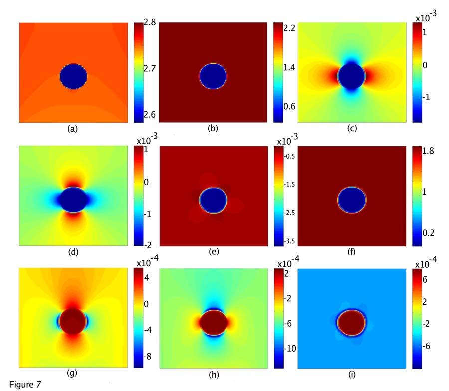
57

58

59