Gradient-domain image processing

Transcription

1 Gradient-domain image processing , , Computational Photography Fall 2018, Lecture 10

2 Course announcements Homework 3 is out. - (Much) smaller than homework 2, but you should still start early to take advantage of bonus questions. - Requires a camera with flash for the second part. Grades for homework 1 have been posted. Make-up lecture will be scheduled soon. - What day does majority of the class prefer? How was Ravi s lecture on Monday? Thoughts on homework 2?

3 Overview of today s lecture Gradient-domain image processing. Basics on images and gradients. Integrable vector fields. Poisson blending. A more efficient Poisson solver. Poisson image editing examples. Flash/no-flash photography.

4 Slide credits Many of these slides were adapted from: Kris Kitani (15-463, Fall 2016). Fredo Durand (MIT). James Hays (Georgia Tech). Amit Agrawal (MERL).

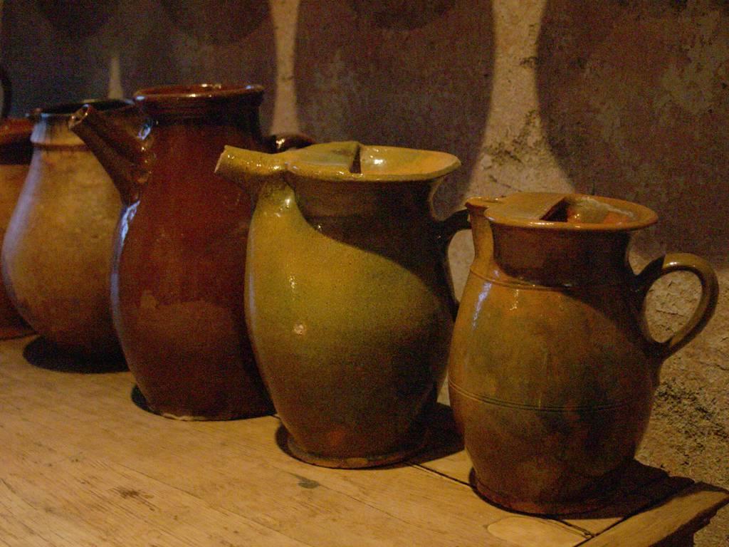
5 Gradient-domain image processing

6 Someone leaked season 8 of Game of Thrones or, more likely, they made some creative use of Poisson blending

7 Application: Poisson blending originals copy-paste Poisson blending

8 More applications Removing Glass Reflections Seamless Image Stitching

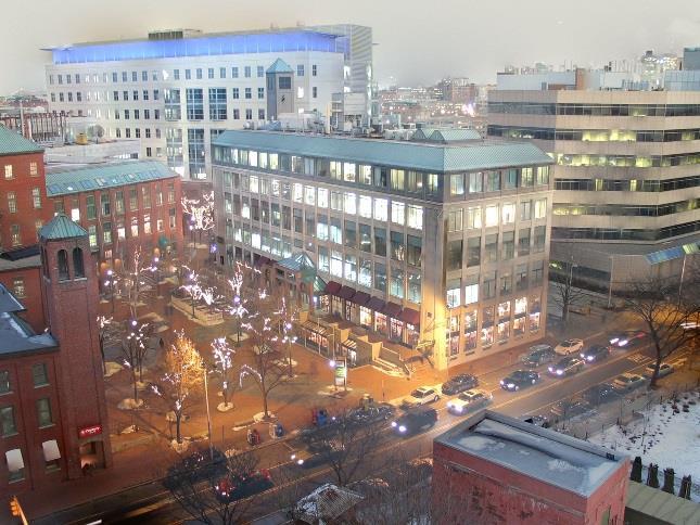
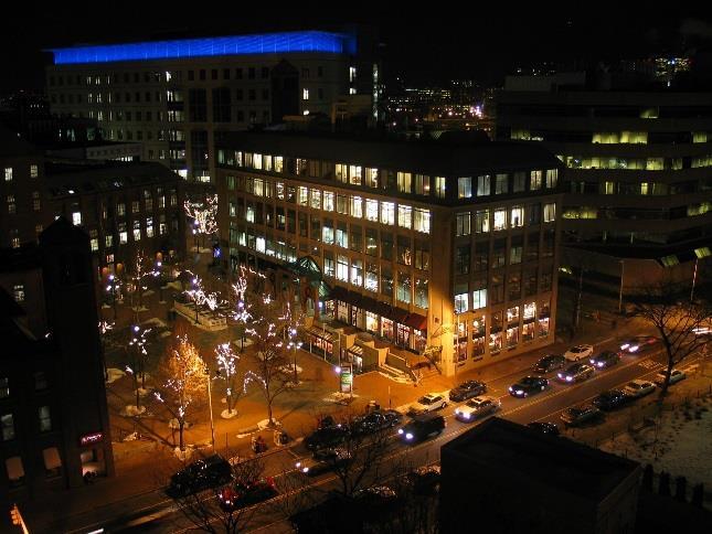
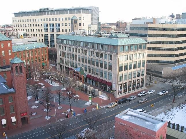
9 Yet more applications Fusing day and night photos Tonemapping

10 Entire suite of image editing tools

11 Main pipeline Estimation of Gradients Images/Videos/ Meshes/Surfaces Non-Integrable Gradient Fields Reconstruction from Gradients Images/Videos/ Meshes/Surfaces Manipulation of Gradients

12 Basics of images and gradients

13 Image representation We can treat images as scalar fields (i.e., two dimensional functions) I(x,y): R 2 R

14 Image gradients Convert the scalar field into a vector field through differentiation. scalar field I I I ( x, y ) : R 2 R vector field I = {, } : R 2 R 2 x y

15 Image gradients Convert the scalar field into a vector field through differentiation. scalar field I I I ( x, y ) : R 2 R vector field I = {, } : R 2 R 2 x y How do we do this differentiation in real discrete images?

16 Finite differences High-school reminder: definition of a derivative using forward difference

17 Finite differences High-school reminder: definition of a derivative using forward difference Alternative: use central difference For discrete signals: Remove limit and set h = 2 How do you efficiently compute this?

18 Finite differences High-school reminder: definition of a derivative using forward difference Alternative: use central difference For discrete signals: Remove limit and set h = 2 What convolution kernel does this correspond to?

19 Finite differences High-school reminder: definition of a derivative using forward difference Alternative: use central difference For discrete signals: Remove limit and set h = ? 1 0-1?

20 Finite differences High-school reminder: definition of a derivative using forward difference Alternative: use central difference For discrete signals: Remove limit and set h = 2 1D derivative filter 1 0-1

21 Image gradients Convert the scalar field into a vector field through differentiation. scalar field I I I ( x, y ) : R 2 R vector field I = {, } : R 2 R 2 x y How do we do this differentiation in real discrete images? Can we go in the opposite direction, from gradients to images?

22 Vector field integration Two core questions: When is integration of a vector field possible? How can integration of a vector field be performed?

23 Integrable vector fields

24 Integrable fields Given an arbitrary vector field (u, v), can we always integrate it into a scalar field I?? I x, y : R 2 R u x, y : R 2 R v x, y : R 2 R such that I x I y x, y x, y = u(x, y) = v(x, y)

25 Curl and divergence Curl: vector operator showing the rate of rotation of a vector field. Curl ( I ) = I Divergence: vector operator showing the isotropy of a vector field. Div ( I ) = I Do you know of some simpler versions of these operators?

26 yy xx y x y x I I y I x I I I div + = + = ), ( Curl and divergence Curl: vector operator showing the rate of rotation of a vector field. Divergence: vector operator showing the isotropy of a vector field. Can you use either of these operators to derive an integrability condition? I I Curl = ) ( xy yx x y y x I I y I x I I I y x = = det

27 Integrability condition Curl of the gradient field should be zero: Curl ( I ) = I I = yx xy 0 What does that mean intuitively?

28 Integrability condition Curl of the gradient field should be zero: Curl ( I ) = I I = yx xy 0 What does that mean intuitively? Same result independent of order of differentiation. I = yx I xy

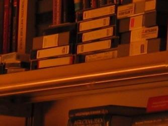
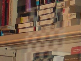
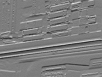
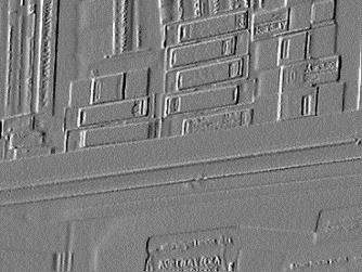
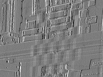
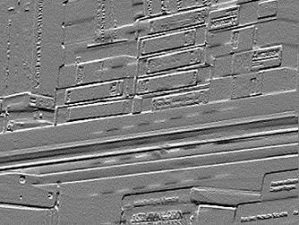
29 Demonstration Image I x I y = How do we compute this? Div(I x, I y ) Curl(I x, I y ) I xy I yx

30 Laplace filter Basically a second derivative filter. We can use finite differences to derive it, as with first derivative filter. first-order 1D derivative filter finite difference second-order finite difference Laplace filter?

31 Laplace filter Basically a second derivative filter. We can use finite differences to derive it, as with first derivative filter. first-order 1D derivative filter finite difference second-order Laplace filter finite difference 1-2 1

32 Vector field integration Two core questions: When is integration of a vector field possible? - Use curl to check for equality of mixed partial second derivatives. How can integration of a vector field be performed?

33 Different types of integration problems Reconstructing height field from gradients Applications: shape from shading, photometric stereo Manipulating image gradients Applications: tonemapping, image editing, matting, fusion, mosaics Manipulation of 3D gradients Applications: mesh editing, video operations Key challenge: Most vector fields in applications are not integrable. Integration must be done approximately.

34 Poisson blending

35 Application: Poisson blending originals copy-paste Poisson blending

36 Key idea When blending, retain the gradient information as best as possible 3 6 source destination copy-paste Poisson blending

37 Poisson blending: 1D example bright dark two signals regular blending blending derivatives

38 Definitions and notation Notation g: source function S: destination Ω: destination domain f: interpolant function f*: destination function add image here Which one is the unknown?

39 Definitions and notation Notation g: source function S: destination Ω: destination domain f: interpolant function f*: destination function add image here How should we determine f? should it look like g? should it look like f*?

40 Interpolation criterion Variational means optimization where the unknown is an entire function Variational problem what does this term do? what does this term do? Recall... Image gradient is this known?

41 Interpolation criterion Variational means optimization where the unknown is an entire function Variational problem gradient of f looks like gradient of g f is equivalent to f* at the boundaries Recall... Image gradient Yes, since the source function g is known

42 This is where Poisson blending comes from Equivalently Poisson equation (with Dirichlet boundary conditions) what does this term do? Gradient Laplacian Divergence

43 Equivalently Poisson equation (with Dirichlet boundary conditions) Laplacian of f same as g Gradient Laplacian Divergence

44 Equivalently Poisson equation (with Dirichlet boundary conditions) so make these guys... the same How can we do this?

45 Equivalently Poisson equation (with Dirichlet boundary conditions) So for each pixel p, do: Or for discrete images: How did we compute the Laplacian?

46 Equivalently Poisson equation (with Dirichlet boundary conditions) So for each pixel p, do: Or for discrete images: Recall... Laplace filter What s known and what s unknown?

47 Equivalently Poisson equation (with Dirichlet boundary conditions) So for each pixel p, do: Or for discrete images: Recall... Laplace filter f is unknown except at the boundary g and its Laplacian are known

48 We can rewrite this as linear equation of N variables one for each pixel in destination In vector form: Linear system of equations What is this? (each pixel adds another sparse row here) How would you solve this? WARNING: requires special treatment at the borders (target boundary values are same as source )

49 Solving the linear system Convert the system to a linear least-squares problem: Expand the error: Minimize the error: Set derivative to 0 Solve for x

50 Solving the linear system Convert the system to a linear least-squares problem: In Matlab: f = A \ b Expand the error: Minimize the error: Set derivative to 0 Solve for x Note: You almost never want to compute the inverse of a matrix.

51 Integration procedures Poisson solver (i.e., least squares integration) + Generally applicable. - Matrices A can become very large. Acceleration techniques: + (Conjugate) gradient descent solvers. + Multi-grid approaches. + Pre-conditioning. + Quadtree decompositions. Alternative solvers: projection procedures. We will discuss one of these when we cover photometric stereo.

52 A more efficient Poisson solver

53 Let s look again at our optimization problem Variational problem gradient of f looks like gradient of g f is equivalent to f* at the boundaries Recall... Image gradient

54 Let s look again at our optimization problem Variational problem gradient of f looks like gradient of g f is equivalent to f* at the boundaries Recall... Image gradient And for discrete images: x y 1 0-1

55 Let s look again at our optimization problem We can use the gradient approximation to discretize the variational problem What are G, f, and v? Discrete problem min f Gf v 2 We will ignore the boundary conditions for now. Recall... Image gradient And for discrete images: x y 1 0-1

56 Let s look again at our optimization problem We can use the gradient approximation to discretize the variational problem Recall... Discrete problem matrix G formed by stacking together discrete gradients min Gf v 2 f vectorized version of the unknown image Image gradient vectorized version of the target gradient field And for discrete images: We will ignore the boundary conditions for now. x y 1 0-1

57 Let s look again at our optimization problem We can use the gradient approximation to discretize the variational problem Recall... Discrete problem matrix G formed by stacking together discrete gradients min Gf v 2 f vectorized version of the unknown image Image gradient vectorized version of the target gradient field And for discrete images: We will ignore the boundary conditions for now. x y 1 0-1

58 Let s look again at our optimization problem Recall... Discrete problem matrix G formed by stacking together discrete gradients min Gf v 2 f vectorized version of the unknown image Image gradient vectorized version of the target gradient field And for discrete images: How do we solve this optimization problem? x y 1 0-1

59 Approach 1: Compute stationary points Given the loss function: we compute its derivative: E f = Gf v 2 E f =?

60 Approach 1: Compute stationary points Given the loss function: we compute its derivative: E f = Gf v 2 E f = GT Gf v and we do what with it?

61 Approach 1: Compute stationary points Given the loss function: we compute its derivative: E f = Gf v 2 E f = GT Gf v and we set that to zero: E f = 0 GT Gf = v What is this matrix?

62 Approach 1: Compute stationary points Given the loss function: we compute its derivative: E f = Gf v 2 E f = GT Gf v and we set that to zero: E f = 0 GT Gf = v It is equal to the Laplacian matrix A we derived previously!

63 Reminder from variational case Poisson equation (with Dirichlet boundary conditions) So for each pixel p, do: Or for discrete images: Recall... Laplace filter What s known and what s unknown?

64 Reminder from variational case linear equation of N variables one for each pixel in destination In vector form: Linear system of equations What is this? (each pixel adds another sparse row here) Same system as: G T Gf = v We arrive at the same system, no matter whether we discretize the continuous Laplace equation or the variational optimization problem.

65 Approach 1: Compute stationary points Given the loss function: we compute its derivative: E f = Gf v 2 E f = GT Gf v and we set that to zero: E f = 0 GT Gf = v Solving this is exactly as expensive as what we had before.

66 Approach 2: Use gradient descent Given the loss function: E f = Gf v 2 we compute its derivative: E f = GT Gf v = Af v r We call this term the residual

67 Approach 2: Use gradient descent Given the loss function: E f = Gf v 2 we compute its derivative: E f = GT Gf v = Af v r We call this term the residual and then we iteratively compute a solution: f i+1 = f i η i r i for i = 0, 1,, N, where η i are positive step sizes

68 Selecting optimal step sizes Make derivative of loss function with respect to E f = Gf v 2 η i equal to zero: E f i+1 = G f i η i r i v 2 E f i+1 r i = v A f i η i r i T r i = 0 η i = ri T r i r i T Ar i

69 Gradient descent Given the loss function: E f = Gf v 2 Minimize by iteratively computing: f i+1 = f i η i r i, r i = v Af i, Is this cheaper than the pseudo-inverse approach? η i = ri T r i r i T Ar i for i = 0, 1,, N

70 Gradient descent Given the loss function: E f = Gf v 2 Minimize by iteratively computing: f i+1 = f i η i r i, r i = v Af i, η i = ri T r i r i T Ar i Is this cheaper than the pseudo-inverse approach? We never need to compute A, only its products with vectors f, r. for i = 0, 1,, N

71 Gradient descent Given the loss function: E f = Gf v 2 Minimize by iteratively computing: f i+1 = f i η i r i, r i = v Af i, η i = ri T r i r i T Ar i Is this cheaper than the pseudo-inverse approach? We never need to compute A, only its products with vectors f, r. Vectors f, r are images. for i = 0, 1,, N

72 Gradient descent Given the loss function: E f = Gf v 2 Minimize by iteratively computing: f i+1 = f i η i r i, r i = v Af i, η i = ri T r i r i T Ar i for i = 0, 1,, N Is this cheaper than the pseudo-inverse approach? We never need to compute A, only its products with vectors f, r. Vectors f, r are images. Because A is the Laplacian matrix, these matrix-vector products can be efficiently computed using convolutions with the Laplacian kernel.

73 In practice: conjugate gradient descent Given the loss function: E f = Gf v 2 Minimize by iteratively computing: f i+1 = f i + η i d i, r i = v Af i, for i = 0, 1,, N d i+1 = r i+1 + β i+1 d i, Smarter way for selecting update directions Everything can still be done β i+1 = ri+1 T r i+1 r i T r i η i = di T r i d i T Ad i using convolutions

74 Does the initialization f 0 matter? Note: initialization

75 Note: initialization Does the initialization f 0 matter? It doesn t matter in terms of what final f we converge to, because the loss function is convex. E f = Gf v 2

76 Note: initialization Does the initialization f 0 matter? It doesn t matter in terms of what final f we converge to, because the loss function is convex. E f = Gf v 2 It does matter in terms of convergence speed. We typically use a multi-grid approach: - Solve an initial problem for a very low-resolution f (e.g., 2x2). - Use the solution to initialize gradient descent for a higher resolution f (e.g., 4x4). - Use the solution to initialize gradient descent for a higher resolution f (e.g., 8x8). - Use the solution to initialize gradient descent for an f with the original resolution NxN.

77 Poisson image editing examples

78 Photoshop s healing brush Slightly more advanced version of what we covered here: Uses higher-order derivatives

79 Contrast problem Loss of contrast when pasting from dark to bright: Contrast is a multiplicative property. With Poisson blending we are matching linear differences.

80 Contrast problem Loss of contrast when pasting from dark to bright: Contrast is a multiplicative property. With Poisson blending we are matching linear differences. Solution: Do blending in log-domain.

81 More blending originals copy-paste Poisson blending

82 Blending transparent objects

83 Blending objects with holes

84 Editing

85 Concealment How would you do this with Poisson blending?

86 Concealment How would you do this with Poisson blending? Insert a copy of the background.

87 Texture swapping

88 How would you do this? Special case: membrane interpolation

89 Special case: membrane interpolation How would you do this? Poisson problem Laplacian problem

90 Flash/no-flash photography

91 Red Eye

92 Unflattering Lighting

93 Motion Blur

94 Noise

95 A lot of Noise

96 Ruined Ambiance

97 Flash No-Flash + Low Noise + Sharp - Artificial Light - Jarring Look - High Noise - Lacks Detail + Ambient Light + Natural Look

98 Image acquisition 1 Lock Focus & Aperture time

99 Image acquisition 1 Lock Focus & Aperture 2 No-Flash Image 1/30 s ISO 3200 time

100 Image acquisition 1 Lock Focus & Aperture 2 3 No-Flash Image 1/30 s ISO 3200 Flash Image 1/125 s ISO 200 time

101 Denoising Result

102 Show a larger result here No-Flash

103 Denoising Result

104 Key idea Denoise the no-flash image while maintaining the edge structure of the flash image How would you do this using the image editing techniques we ve learned about?

105 Denoising with bilateral filtering noisy input bilateral filtering median filtering

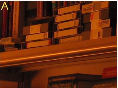
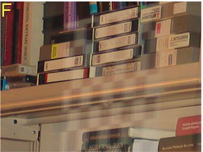
106 Denoising with bilateral filtering However, results still have noise or blur (or both) ambient flash Bilateral filter

107 Denoising with joint bilateral filtering In the flash image there are much more details Use the flash image F to find edges

108 Denoising with joint bilateral filtering Bilateral filter The difference Joint Bilateral filter

109 Not all edges in the flash image are real Can you think of any types of edges that may exist in the flash image but not the ambient one?

110 Not all edges in the flash image are real shadows specularities May cause over- or under-blur in joint bilateral filter We need to eliminate their effect

111 Detecting shadows Observation: the pixels in the flash shadow should be similar to the ambient image. Not identical: 1. Noise. 2. Inter-reflected flash. Compute a shadow mask. Take pixel p if is manually adjusted Mask is smoothed and dilated

112 Detecting specularities Take pixels where sensor input is close to maximum (very bright). Over fixed threshold Create a specularity mask. Also smoothed. M the combination of shadow and specularity masks: Where M p =1, we use A Base. For other pixels we use A NR.

113 Detail transfer Denoising cannot add details missing in the ambient image Exist in flash image because of high SNR We use a quotient image: Reduces the effect of noise in F Multiply with A NR to add the details Masked in the same way Bilateral filtered Why does this quotient image make sense for detail?

114 Detail transfer Denoising cannot add details missing in the ambient image Exist in flash image because of high SNR We use a quotient image: Reduces the effect of noise in F

115 Full pipeline

116 Demonstration ambient-only joint bilateral and detail transfer

117 Can we do similar flash/no-flash fusion tasks with gradient-domain processing?

118 Removing self-reflections and hot-spots Ambient Flash

119 Removing self-reflections and hot-spots Ambient Flash Face Hands Tripod

120 Removing self-reflections and hot-spots Ambient Result Reflection Layer Flash

121 Idea: look at how gradients are affected Same gradient vector direction Flash Gradient Vector Ambient Gradient Vector Ambient Flash No reflections

122 Idea: look at how gradients are affected Different gradient vector direction Reflection Ambient Gradient Vector Flash Gradient Vector Ambient Flash With reflections

123 Idea: look at how gradients are affected Different gradient vector direction Reflection Ambient Gradient Vector Flash Gradient Vector Ambient Flash With reflections

124 Gradient projections Residual Gradient Vector Flash Gradient Vector Result Gradient Vector Ambient Flash Result Residual

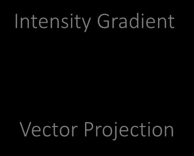
125 Flash/no-flash with gradient-domain processing X Y Flash Intensity Gradient Result X 2D Integration 2D Result Y Integration X Vector Projection Result Y Ambient

126 Flash

127 No-Flash

128 No-Flash

129 Result

130 Flash

131 No-Flash

132 No-Flash

133 Result

134 Flash

135 No-Flash

136 Flash

137 No-Flash

138 Result

139 References Basic reading: Szeliski textbook, Sections 3.13, 3.5.5, 9.3.4, Pérez et al., Poisson Image Editing, SIGGRAPH The original Poisson Image Editing paper. Agrawal and Raskar, Gradient Domain Manipulation Techniques in Vision and Graphics, ICCV 2007 course, A great resource (entire course!) for gradient-domain image processing. Petschnigg et al., Digital photography with flash and no-flash image pairs, SIGGRAPH Eisemann and Durand, Flash Photography Enhancement via Intrinsic Relighting, SIGGRAPH The first two papers exploring the idea of photography with flash and no-flash pairs, both using variants of the joint bilateral filter. Agrawal et al., Removing Photography Artifacts Using Gradient Projection and Flash-Exposure Sampling, SIGGRAPH A subsequent paper on photography with flash and no-flash pairs, using gradient-domain image processing. Additional reading: Georgiev, Covariant Derivatives and Vision, ECCV An paper from Adobe on the version of Poisson blending implemented in Photoshop s healing brush. Elder and Goldberg, Image editing in the contour domain, PAMI One of the very first papers discussing gradient-domain image processing. Szeliski, Locally adapted hierarchical basis preconditioning, SIGGRAPH A standard reference on multi-grid and preconditioning techniques for accelerating the Poisson solver. Bhat et al., Fourier Analysis of the 2D Screened Poisson Equation for Gradient Domain Problems, ECCV A paper discussing the (Fourier) basis projection approach for solving the Poisson integration problem. Bhat et al., GradientShop: A Gradient-Domain Optimization Framework for Image and Video Filtering, ToG A paper describing gradient-domain processing as a general image processing paradigm, which can be used for a broad set of applications beyond blending, including tone-mapping, colorization, converting to grayscale, edge enhancement, image abstraction and non-photorealistic rendering. Krishnan and Fergus, Dark Flash Photography, SIGGRAPH A paper proposing doing flash/no-flash photography using infrared flash lights. Kettunen et al., Gradient-domain path tracing, SIGGRAPH In addition to editing images in the gradient-domain, we can also directly render them in the gradient-domain. Tumblin et al., Why I want a gradient camera? CVPR We can even directly measure images in the gradient domain, using so-called gradient cameras.