AUTOMATIC CONTROL ENGINEERING HINCHEY

Transcription

1 AUTOMATIC CONTROL ENGINEERING HINCHEY

2 AUTOMATIC CONTROL ENGINEERING FEEDBACK CONTROL CONCEPT The sketch on the next page shows a typical feedback or error driven control system. What has to be controlled is generally referred to as the plant. What the plant is doing is known as its response. What it should be doing is known as the command. The plant receives a control signal from a drive and a disturbance signal from the surroundings. The goal is to pick a controller that can make the response follow closely command signals but reject disturbances. The controller acts on an error signal: this is command minus some measure of the response. This is why it is usually called error driven control. Two types of error driven control are PID and Switching. PID stands for proportional integral derivative. Proportional generates a signal which is proportional to error. Integral generates a signal which is proportional to the integral of the error. Derivative generates a signal which is proportional to the rate of change of error. Switching generally gives out signals with constant levels. AUTONOMOUS UNDERWATER VEHICLE DEPTH CONTROL To illustrate some error driven control strategies we will consider the task of controlling the submergence depth of a small autonomous underwater vehicle or auv. According to Newton's Second Law of Motion, the equation governing its up and down motion is: M d 2 R/dt 2 = B + D - W

3

4

5 where R is the depth of the auv, M is its overall mass, B is the control force from the propulsion system, D is a disturbance load caused for example by sudden weight changes and W is a drag load. Drag load has two components: wake drag and wall drag: W = X dr/dt dr/dt + Y dr/dt where X and Y account mainly for the size and shape of the auv. A simple model of the propulsion system is: J db/dt + I B = Q where Q is the control signal. There are two basic types of propulsion systems that could be used to move the auv up and down. One is an air/water ballast tank. In this case, the control signal Q would produce a change in buoyancy and J would account for the fact that this is caused by a flow: I would be zero. If J was very large, the control force B would build up very slowly. The other type of propulsion system uses motor driven propellors to generate B. Usually, for protection, these would be located inside a duct. In this case, I would account for the size and shape of the blades and duct, while J would account for things like rotor inertia. Again, if J was very large, the control force B would build up very slowly. One could determine J and I experimentally. The PID error driven strategy lets the control signal Q be:

6 Q = KP E + KI Edτ + KD de/dt where E = C - R is the depth error and KP KI KD are gains: C is the command depth. Usually, gains are constants. However, they can be made a function of the state of the system or its surroundings. In this case, control is said to be adaptive. Imagine the auv is at the water surface and it suddenly commanded to go to some constant command depth C. Assume that there is a disturbance with a constant level D acting downward. Also assume the auv is using motor driven propellors for propulsion. Proportional by itself would cause the propellors to spin in such a way that the auv would move towards the command depth. The amount of spin would be proportional to depth error. When the auv reaches the command depth, the proportional control signal would be zero. If the auv was held at the command depth, its propellors would stop spinning. The disturbance would cause the auv to stop below the command depth. This offset would be such that the propellors generate just enough upward force to balance the downward disturbance. The offset would be DI/KP. When D is known, something called feedforward compensation can be used to get rid of the offset. Basically, we measure D and subtract ID from Q in the drive equation. When motions settle down, the drive gives out an extra signal minus D which cancels D. But we must know D. Another way to get rid of the offset is to give the auv a false

7 command C *. If the false command C * was set at [C-DI/KP], the auv would end up at C. It would hang below C * by DI/KP and thus end up at C. If the gain KP was very large, offsets such as DI/KP would probably be tolerable. However, large gain would generate very large Q when the depth is well away from the command depth. Very large Q could burn out drives. To avoid this, a limit is usually put on the magnitude of Q. In this case, the control is referred to as proportional with saturation. If the disturbance was greater than the saturation limits, then control would be impossible. Integral by itself would cause the propellors to spin in such a way that the auv would move towards the command depth. The amount of spin would be proportional to the integral of depth error. As the auv moves towards the command depth, the propellors would spin faster and faster. Obviously, this would cause the auv to overshoot the command depth. Because of these overshoots, integral cannot be used alone. The good thing about integral is, if the system is stable, it gives zero offsets. If the auv was held with positive depth error, the integral control signal would get bigger and bigger. This is known as integral windup. If it was released after a long time, it would take a very large integrated negative error to cancel out the windup due to integrated positive error. A simple way to avoid integral windup is to activate integral only within a band surrounding the command depth. All we need is for the band to be wide enough for proportional to get the auv within the band so that integral can then home it into the command depth. Derivative like integral cannot be used alone. Assume that the

8 command C is a constant, and let the auv be stopped far away from the command depth. In this case, de/dt would be zero. So, the controller would not generate a force to move the auv to the command depth. Derivative mimics drag load and helps motions settle down. It generates a control signal which opposes motion. Something called rate feedback could also be used to help make motions settle down. The controller would act on depth error E minus a constant times the depth rate dr/dt. Substitution into the governing equations shows that rate feedback mimics drag. Note that derivative could be used to make the auv move at a constant speed: dc/dt is made a constant. Drag and the dr/dt part of de/dt would tend to limit speed. With all three components of PID acting together, as soon as the auv passes through the command depth, proportional would tend to counteract integral. Also, proportional would get the auv closer to the command depth faster, so it would limit integral windup. Derivative would help counteract overshoots. The auv would home in quickly on the command depth with minimal overshoots. So, we get the good characteristics of all three controllers. There are many types of switching control. They often have trouble with overshoots. Basic relay switching is the simplest. It would try to make the propellors rotate at a constant speed: the direction of rotation would depend on the sign of depth error. Relay with deadband would allow the auv to drift once it gets inside a band surrounding the command depth. The propulsion device

9 would be shut down and drag load would cause the auv to slow down. Relay with hysteresis would reverse the direction of control before the auv gets to the command depth. In this case, the propulsion device would act as a brake. A bias signal could be added to counteract disturbances. Propulsion system dynamics would cause the control force to lag the control signal. The amount of lag depends on how large J is relative to I. Consider the case where proportional control is acting alone and the error is initially positive. For a slowly reacting propulsion system, positive error would cause a positive control force to gradually build up. As it builds up, this force would move the auv towards the command depth. However, when the auv gets to the command depth, because of lag, the control force would still be positive, and this would cause overshoot. In some cases, these overshoots would settle down. In other cases, they would not settle down but would limit because of wake drag. Control signals for an auv would be generated within a computer control loop. The loop period must be much smaller than the basic period of auv motion: otherwise severe overshoots could develop. If the auv was controlled remotely by a computer onboard a ship, the time taken for the depth signal to travel from the auv to the ship and the time taken for the drive signal to travel back from the ship to the auv could cause overshoots, because the auv would be responding to past error not present error.

10 SUBSEA ROBOT SPRING/DASHPOT PID ANALOGY Equations governing subsea robot depth motion are: M d 2 R/dt 2 + X dr/dt dr/dt + Y dr/dt = B + D J db/dt + I B = Q Q = K P (C-R) + K I (C-R)dτ + K D (dc/dt-dr/dt) Let the drive be a propellor in a duct driven by a DC motor. For most of what follows, we will assume that the drive is fast acting, so that J is approximately zero. In this case, B = K P /I (C-R) + K I /I (C-R)dτ + K D /I (dc/dt-dr/dt) B = K P (C-R) + K I (C-R)dτ + K D (dc/dt-dr/dt) We will also assume that the robot is initially at one depth and it is suddenly commanded to go to another depth. When proportional control is acting alone, the control force B is a linear function of depth error. This pulls the robot towards the command depth. As the robot approaches the command depth, the propellor slows down. Note that a spring with its ends attached to the robot and the command depth would move the robot the same way. Because the drive is spring like, disturbances D cause the robot to settle down away from the command depth. When integral control is acting alone, the control force B gradually builds up and pulls the robot towards the command depth. As the robot approaches the command depth, the propellor goes faster and faster. This causes the robot to

11 overshoot the command depth. As soon as it overshoots, the control force starts to decrease: meaning the propellor starts to slow down. It takes time for the control force to go to zero. Beyond this point, the control force changes sign and acts initially like a brake and causes the robot to stop and then start back towards the command depth. Again, when it reaches the command depth, it overshoots it. These overshoots do not settle down. If they did, B would equal minus D and R would equal C. One could replace the integral drive with a spring with one end attached to the robot and the other end free to move. Initially the free end moves towards the command depth. This causes the spring to stretch and pull the robot towards the command depth. The spring stretching mimics the integration of error. The spring keeps stretching until the robot overshoots the command depth. Then, it gradually slackens. It takes time for the spring to totally slacken so it pulls the robot beyond the command depth. When the spring is totally slack, the free end starts back towards the command depth. In this case, the spring acts initially like a brake and causes the robot to stop and then start back towards the command depth. With proportional and integral acting together it is possible for the robot to settle at the command depth. Proportional suppresses the overshoots caused by integral and integral gets rid of offsets. Derivative control is not spring like. The equation for B shows that it instead mimics a dashpot. When the drive is slow acting, control actions are not instantaneous. This can cause severe overshoots.

12 CAR/DRIVER PID ANALOGY Imagine a car at position A on a straight road that is suddenly commanded to go to position B on the same road. A proportional driver would suddenly depress the gas peddle down to some level. This would cause the car to gradually pick up speed. As the car moves towards B, the driver would depress the gas peddle less and less. The amount of depression would be a linear function of position error or distance between B and the car position. When the car reaches B, peddle depression would be zero. Because of its momentum, the car would overshoot B. As soon as it does so, the driver would suddenly put the car into reverse and depress the gas peddle an amount again dependent on position error. This would cause the car to gradually come to a stop and reverse direction back towards B. If there was no wind and the road was horizontal, wake drag and drive friction would gradually make the car come to rest at B. Otherwise, it would come to rest away from B. An integral driver starting at A would gradually depress the gas peddle based on the integral of position error. This would move the car towards B but at a faster and faster speed. When the car reaches B, peddle depression would be maximum. Obviously, the car would overshoot B. As soon as it does so, the driver would gradually depress the gas peddle less and less. Basically, the position error would now be negative, and

13 integrated error would gradually decrease. When it reaches zero, the peddle depression would also be zero, and the driver would suddenly put the car into reverse and gradually depress the gas peddle again based on the integral of position error. This would cause the car to gradually come to a stop and reverse direction back towards B. When the car reaches B, it would again overshoot. The car would never settle at B but would oscillate back and forth at an amplitude dependent on wake drag and drive friction. The mean position error would be zero, even when there was wind or the road was not horizontal. A proportional plus integral driver could make the car settle at B, even when there was wind or the road was not horizontal. The proportional part would bring the car close to B before the integral part could build up too much signal. The integral part would then home the car into B. Whereas the proportional plus integral driver would work only the gas peddle, a proportional plus integral plus derivative driver would also use the brake. The derivative part would apply the brake an amount based on speed. This would help control overshoots if they are a problem. Driver reaction time could cause severe overshoots. Its control is based on past error not present error.

14 ZIEGLER NICHOLS GAINS Ziegler and Nichols, through a series of experiments on simple systems, developed criteria for picking gains in a controller that would give good tracking performance. For a system that can be made unstable with proportional acting alone, the procedure they recommend is as follows. With proportional acting alone, increase its gain until the system becomes borderline stable. Let the borderline gain be KP: let its period be TP. According to Ziegler and Nichols, reasonable PID gains are: KP = 0.6*KP KI = KP/TI KD = KP*TD TI = 0.5*TP TD = 0.125*TP When only proportional and integral are acting, they recommend the following PI gains: KP = 0.45*KP KI = KP/TI TI = 0.83*TP When only proportional is acting, they recommend: KP = 0.5*KP

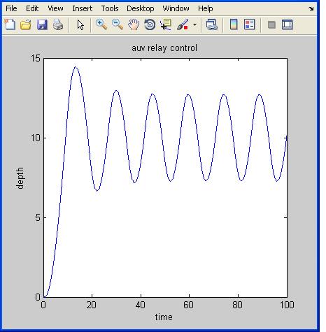
15 AUTONOMOUS UNDERWATER VEHICLE ZIEGLER NICHOLS GAINS To illustrate a procedure for getting Ziegler Nichols gains, we will consider the task of controlling the submergence depth of a small autonomous underwater vehicle or auv. According to Newton's Second Law of Motion, the equation governing the up and down motion of the auv is: M d 2 R/dt 2 = B + D - W where R is the depth of the auv, M is its overall mass, B is the control force from the propulsion system, D is a disturbance load caused for example by sudden weight changes and W is a drag load consisting of wake drag and wall drag: W = X dr/dt dr/dt + Y dr/dt where X and Y account for the size and shape of the auv. Here we linearize the drag to get: W = N dr/dt A simple model of the propulsion system is: J db/dt + I B = Q where Q is the control signal: J and I are drive constants.

16 The PID error driven strategy lets the control signal Q be: Q = KP E + KI Edτ + KD de/dt where E = C - R is the depth error and KP KI KD are the controller gains: C is the command depth. To get Ziegler Nichols gains, we start by assuming only proportional is active. Manipulation of the governing equations gives: J [ M d 3 R/dt 3 + N d 2 R/dt 2 - dd/dt] + I [ M d 2 R/dt 2 + N dr/dt - D ] = KP C - KP R We then assume that C and D are both constants and that the auv is undergoing a limit cycle oscillation for which R = Ro + R Sin [ t] Substitution into the modified drive equation gives - J M 3 R Cos[ t] - J N 2 R Sin[ t] - I M 2 R Sin[ t] + I N R Cos[ t] - I Do = KP Co - KP Ro - KP R Sin[ t] This equation is of the form:

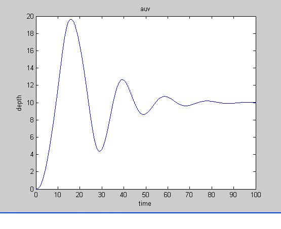
17 i Sin[ t] + j Cos[ t] + k = 0 Mathematics requires that i=0 j=0 k=0: - J N 2 - I M 2 + KP = 0 - J M 3 + I N = 0 + I Do + KP Co - KP Ro = 0 Manipulation of these equations gives Ro = Co + I Do / KP 2 = [I N] / [J M] KP = [J N + I M] 2 = [J N + I M] [I N] / [J M] For the illustration we let : M=50 N=50 J=0.5 I=0.1. The above equations give =0.447, KP=6 and TP=14. Substitution into the Ziegler Nichols gains equations gives: KP = 3.6; KI = 0.54; KD = 6.3. An m code for the auv is given below. This is followed by a Ziegler Nichols response generated by the code. A SIMULINK Block diagram follows the m code response. It gives basically the same response as the code.

18

19

20

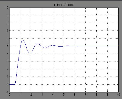
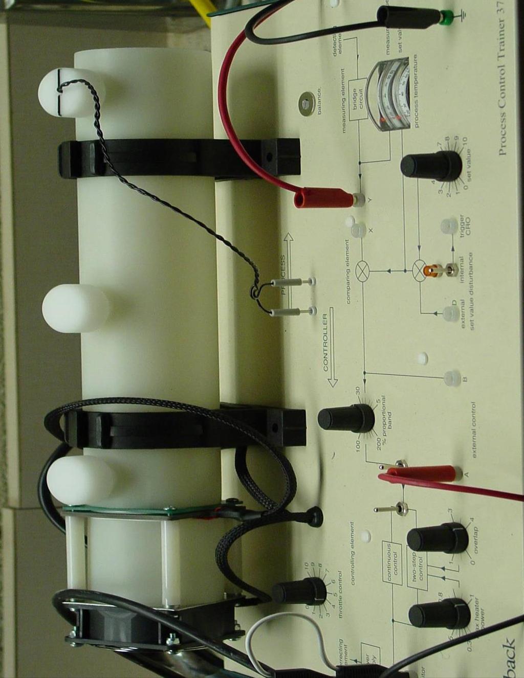
21 PIPE FLOW SETUP ZIEGLER NICHOLS GAINS To illustrate a procedure for getting Ziegler Nichols gains, we will consider the task of controlling the temperature of the air flowing down the pipe in the lab pipe flow setup. Basically the setup consists of a fan which draws air from atmosphere and sends it down a pipe. A heater just downstream of the fan is used to heat the air. It receives a signal from a controller. The temperature of the air at the pipe exit is measured by a thermistor. The governing equations are: X dr/dt + Y R = H + D A dh/dt + B H = Z Q Q = KP E + KI Edτ + KD de/dt E = C - R where R is the temperature of the air at the heater, R is the temperature of the air at the sensor, C is the command temperature, E is the temperature error, Q is the control signal, H is the heat generated by the heater, D is a disturbance heat and KP KI KD are the controller gains. Note that R is what R was T seconds back in time: T is the time it takes for the air to travel down the pipe.

22 To get Ziegler Nichols gains, we start by assuming only proportional is active. Manipulation of the governing equations gives: A [ X d 2 R/dt 2 + Y dr/dt - dd/dt] + B ( X dr/dt + Y R - D) = Z KP C - Z KP R We then assume that C and D are both constants and that the setup is undergoing a limit cycle oscillation for which R = Ro + R Sin [ t] R = Ro + R Sin [ (t-t)] Substitution into the modified drive equation gives - A X 2 R Sin[ t] + A Y R Cos[ t] + B X R Cos[ t] + B Y Ro + B Y R Sin[ t] - B Do = Z KP Co - Z KP Ro - Z KP R Sin[ (t-t)] A trigonometric identity gives Sin[ (t-t)] = Sin[ t] Cos[ T] - Cos[ t] Sin[ T] Substitution into the modified drive equation gives an equation of the form i Sin[ t] + j Cos[ t] + k = 0

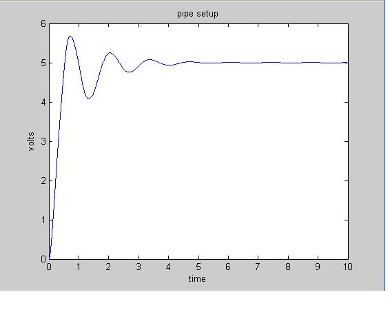
23 Setting i=0 and j=0 and k=0 gives - A X 2 + B Y + Z KP Cos[ T] = 0 A Y + B X - Z KP Sin[ T] = 0 B Y Ro - B Do - Z KP Co + Z KP Ro = 0 Manipulation of the first two equations gives KP = [A X 2 - B Y] / [Z Cos[ T]] KP = [A Y + B X ] / [Z Sin[ T]] Sin[ T]/Cos[ T] = Tan[ T] = [A Y + B X ] / [A X 2 - B Y] The last equation gives. Once is known we can then solve for KP. For the illustration, we let: X=0.25 Y=1.0 A=0.1 B=1.0 Z=1.0 T=0.5. The above equations give =3.97, KP=1.5 and TP=1.58. Substitution into the Ziegler Nichols gains equations gives: KP=0.9; KI=1.2; KD=0.17. An m code for the setup is given below. This is followed by a Ziegler Nichols response. A SIMULINK Block diagram follows the response. It gives basically the same response as the code.

24

25

26

27 COMPUTER SIMULATION OF CONTROL SYSTEMS PREAMBLE Simulation allows one to study the behavior of a system before it is actually constructed. This can serve as an aid to system design. Simulations are inexpensive and easy to put together. They can handle all sorts of phenomena. These include transport lag and computer loop rate phenomena. Simulations can also handle multiple strong nonlinearities. They are often used as a check on more conventional analysis. However, simulations are like experiments. For complex systems, it is hard to make sense of responses. Before digital computers were developed, systems were simulated using analog electronics. When digital computers became common place, simulations made use of time stepping procedures. Basically, these follow local slopes or rates step by step in time. Special software packages based on these procedures have been developed. Probably, the popular package is SIMULINK under MATLAB.

28 AUTONOMOUS UNDERWATER VEHICLE TIME STEPPING SIMULATION To illustrate time stepping we will consider the task of controlling the submergence depth of a small autonomous underwater vehicle or auv. The governing equations are: M d 2 R/dt 2 = B + D - W W = X dr/dt dr/dt + Y dr/dt J db/dt + I B = Q Q = KP E + KI Edτ + KD de/dt E = C - R where R is the depth of the auv, M is its overall mass, B is the control force from the propulsion system, D is a disturbance load caused for example by sudden weight changes, W is a drag load consisting of wake drag and wall drag, E is the depth error, C is the command depth, M X Y J I are process constants and KP KI KD are the controller gains.

29 Manipulation of the governing equations gives dr/dt = U du/dt = (B + D - W) / M W = X U U + Y U db/dt = (Q - I B) / J Q = KP E + KI Edτ + KD de/dt E = C - R Application of time stepping gives RNEW = ROLD + t * UOLD UNEW = UOLD + t * (BOLD + DOLD - WOLD) /M WOLD = X UOLD UOLD + Y UOLD BNEW = BOLD + t * (QOLD - I BOLD) / J QOLD = KP EOLD + KI EOLD t + KD EOLD/ t EOLD = COLD - ROLD An m code for the auv is given below. This is followed by a Ziegler Nichols response generated by the code.

30

31

32 PIPE FLOW SETUP TIME STEPPING SIMULATION To illustrate time stepping we will consider the task of controlling the temperature of air flowing down a pipe. The setup is shown on the next page. The governing equations are: X dr/dt + Y R = H + D A dh/dt + B H = Z Q Q = KP E + KI Edτ + KD de/dt E = C - R where R is the temperature of the air at the heater, R is the temperature of the air at the sensor, C is the command temperature, E is the temperature error, Q is the control signal, H is the heat generated by the heater, D is a disturbance heat (plus or minus), X Y A B Z are process constants and KP KI KD are the controller gains. Note that R is what R was T seconds back in time: T is the time it takes for the air to travel down the pipe.

33

34 Manipulation of the governing equations gives dr/dt = (H + D - Y R) / X dh/dt = (Z Q - B H) / A Q = KP E + KI Edτ + KD de/dt E = C - R Application of time stepping gives RNEW = ROLD + t * (HOLD + DOLD - Y ROLD) / X HNEW = HOLD + t * (Z QOLD - B HOLD) / A QOLD = KP EOLD + KI EOLD t + KD EOLD/ t EOLD = COLD - ROLD An m code for the setup is given below. This is followed by a Ziegler Nichols response generated by the code.

35

36

37 SIMULINK CONTROL SYSTEM SIMULATION SIMULINK makes use of a block diagram representation of the system. One activates SIMULINK by typing SIMULINK and pressing enter in the main MATLAB window. Blocks are formed by picking blocks from groups of blocks in the main SIMULINK window. The group labeled SOURCES contains blocks that could be used for commands and disturbances. The group labeled SINKS contains blocks that could be used for display of responses. The group labeled CONTINUOUS contains many common transfer functions and state space blocks. The group labeled DISCRETE contains blocks that could be used to mimic loop rate phenomena. The group labeled MATH contains blocks for things like summation junctions and gains. The group labeled NONLINEAR contains various types of nonlinearities and switching controllers. Many of the switching controllers can be formed using LOOK UP TABLE under the group of blocks labeled FUNCTIONS & TABLES. The PID controller can be found under ADDITIONAL LINEAR under SIMULINK EXTRAS under BLOCK SETS & TOOL BOXES.

38 Block diagram construction makes extensive use of the click and drag functions of the left and right buttons of the mouse. To illustrate the construction, imagine you have an empty MINE window open on the screen. From the SIMULINK window, double left click on the SOURCES icon. Then, from its window, left click on the STEP block and drag it to the MINE window. All other blocks can be moved this way. You can also use COPY and PASTE. To move blocks around in the MINE window, just left click and drag them. You can also use CUT and PASTE. To join blocks with lines, you again use left click and drag. To create break lines, you use right click on the break point and drag. To change parameters, double left click on the block to activate a block menu. To run a simulation, first pick PARAMETERS under SIMULATION to set things like ODE integration scheme. Then, pick START under SIMULATION to run the simulation. SIMULINK block diagrams for AUV Depth Control and Pipe Flow Temperature Control are attached. Also attached are Ziegler Nichols responses of each system to a step in command.

39 AUTONOMOUS UNDERWATER VEHICLE To illustrate SIMULINK we will consider the task of controlling the submergence depth of a small autonomous underwater vehicle or auv. The governing equations are: M d 2 R/dt 2 + N dr/dt = B + D J db/dt + I B = Q Q = KP E + KI Edτ + KD de/dt E = C - R Laplace transformation gives [ M S 2 + N S ] R = B + D [ J S + I ] B = Q Q = [KP + KI/S + KD S ] E Transfer functions are R / [ B + D ] = 1 / [ M S 2 + N S ] B / Q = 1 / [ J S + I ] Q / E = [KP + KI/S + KD S ]

40

41

42 PIPE FLOW SETUP To illustrate SIMULINK we will consider the task of controlling the temperature of air flowing down a pipe. The governing equations are: X dr/dt + Y R = H + D A dh/dt + B H = Z Q Q = KP E + KI Edτ + KD de/dt E = C - R Laplace transformation gives [ X S + Y ] R = H + D [ A S + B ] H = Z Q Q = [KP + KI/S + KD S ] E E = C - R R = e -TS R Transfer functions are R / [ H + D ] = 1 / [ X S + Y ] H / Q = Z / [ A S + B ] Q / E = [KP + KI/S + KD S ] E = C - R R / R = e -TS

43

44

45 CONTROL SYSTEM STABILITY The standard form block diagram is This gives the transfer function O / I = G / [1 + GH] A unit impulse jars a system from a rest state and the motion thereafter is nonforced. It is a good input to test stability. For a unit impulse input I=1 and the response becomes

46 O = H = G / [1 + GH] = N / D where N and D are polynomials. The characteristic equation is D=0. Partial Fraction Expansion (PFE) gives O = / [S - ] where each is a root of the characteristic equation. Inverse Laplace Transformation (ILT) gives O = e + t The G and H transfer functions can be written as G = A/B H=X/Y GH = A/B X/Y = AX/BY = N/D where A B X Y N D are polynomials. In this case O = G / [1+GH] = A/B / [1+A/B X/Y] = AY / [BY + AX] = N / D

47 This shows that D = N + D The [1+GH] function is: 1 + GH = 1+ N/D = [N+D] / D = D / D Setting D equal to 0 gives the overall characteristic equation. Setting D equal to 0 gives the characteristic equation for the sub systems. The [1+GH] function can be factored to give: π [S-Z] / π [S-P] where the symbol π indicates product. Zeros Z are values of S which make [1+GH] zero. Poles P are values of S which make [1+GH] infinite. Note that each [S-Z] factor is basically a vector with its origin at Z. Similarly each [S-P] factor is basically a vector with its origin at P.

48 NYQUIST CONCEPT The Nyquist Concept starts by surrounding the entire unstable half of the S plane with a clockwise contour. The [1+GH] function is basically a vector made from zero and pole factors which are also vectors: π [S-Z] / π [S-P] = R Θ When the tip of the S vector moves clockwise around the Nyquist contour, zeros Z inside it cause clockwise rotations of [1+GH] while poles P inside it cause counter clockwise rotations. Only zeros and poles inside cause such rotations: zeros and poles outside only cause [1+GH] to nod up and down. The sketches on the next page show a complex conjugate pair of roots inside the Nyquist contour and the corresponding [1+GH] plot. As can be seen, the [1+GH] vector rotates twice clockwise as the tip of the S vector moves clockwise around the Nyquist contour. These clockwise rotations are caused by the two unstable zeros inside the contour. Subtracting one from [1+GH] and its origin gives GH and minus one. One can use a GH plot with a radius drawn from minus one to determine rotations.

49

50

51 ROOT LOCUS CONCEPT When S is a Z or root of the overall characteristic equation, [1+GH] is equal to zero. This implies that GH is equal to minus unity: GH = -1. This means its magnitude is unity and its angle is plus or minus 180 degrees. So any S which satisfies these constraints is a root of the overall characteristic equation. To determine borderline proportional gain and period the angle constraint is used to determine the period and the magnitude constraint is used to determine the gain. Consider the GH function GH = K X [ (S-v) (S-w) ] / [ (S-a) (S-b) (S-c) ] Its poles and zeros are shown in the sketch. The location of the square point in the sketch is adjusted to satisfy the angle constraint: α + β - ε - κ - σ = ±180 The magnitude constraint requires that K [X V W] / [A B C] = 1 where the lengths V W A B C can be measured. Manipulation gives K = [A B C] / [X V W]

52

53 CONTROL SYSTEM DESIGN STABILITY MARGINS The degree of stability of a control system depends on how close the GH plot is to the minus one point. Two measures of closeness are the gain margin GM and the phase margin PM. Engineering experience suggests that GM should be at least 2 and PM should be at least 30 o. WEDGE CIRCLE REGION Most systems have a dominant pair of roots which control how stable it is. Theory shows that the damping factor associated with these roots is constant along radial lines drawn from the origin in the S plane while the undamped natural frequency is constant along semi circles with center at the origin of the S plane. The wedge circle region is where roots should be located to get good damping and speed of response.

54

55

56 OVERVIEW OF NYQUIST The Nyquist procedure is based on the 1+GH function: 1 + GH = 1 + N/D = (N+D)/D = D/D Γ (S-Z 1 ) (S-Z 2 ) ::::: (S-Z n ) = = R Θ (S-P 1 ) (S-P 2 ) ::::: (S-P m ) It is basically a vector made from zero and pole factors which are also vectors. When the tip of the S vector moves clockwise around the Nyquist contour, zeros Z inside it cause clockwise rotations of 1+GH while poles P inside it cause counterclockwise rotations. Only zeros and poles inside cause such rotations: zeros and poles outside only cause 1+GH to nod up and down. In the 1+GH plane R is drawn from the origin. In the GH plane, R is drawn from the minus one point. We want to find the number of unstable zeros N Z. From the GH plot, one gets the net clockwise rotations of the GH vector N. The net clockwise rotations N must be equal to the number of unstable zeros N Z minus the number of unstable poles N P. From the GH function, one gets the number of unstable poles N P. Manipulation gives N Z : N = N Z - N P N Z = N + N P

57

58

59 NYQUIST ILLUSTRATION Consider the case where there two unstable zeros in the right half of the S plane and all other zeros and poles are far into the left half of the S plane. Now surround the unstable zeros by a clockwise contour as shown on the next page. When we map points on this contour to the 1+GH plane, we get the contour two pages over. When we draw a vector with radius R and angle to the contour in the 1+GH plane and count the number of times it rotates clockwise as we move around the contour in the S plane, we get two clockwise rotations. These rotations are caused by the unstable zeros. Nyquist allows us to determine the number of unstable zeros without having to find their exact locations.

60

61

62 SIGNIFICANCE OF GH EQUAL TO MINUS ONE Consider the case where only proportional control is being used and the GH plot passes through the minus one point in the GH plane. If GH=-1 then 1+GH=0. This implies that at this point S=Z: in other words, it is a root of the overall characteristic equation. But along the GH plot S=±jω. So Z=±jω. So there is a complex conjugate pair of roots of the overall characteristic equation on the imaginary axis in the S plane. This means the system is borderline stable and the gain K is the borderline stable gain K and the frequency ω is the borderline stable frequency ω. The borderline stable period is T=2Π/ω.

63

64 OPEN LOOP FREQUENCY RESPONSE A GH plot is basically a polar open loop frequency response plot. Consider the case where only proportional control is being used. When GH=-1, a command sine wave produces a response which has the same magnitude as the command but is 180 o out of phase. If the command was suddenly removed and the loop was suddenly closed, the negative of the response would take the place of the command and keep the system oscillating. The system would be borderline stable with gain K. If the gain was bigger than K, the command would produce a response bigger than itself. When this takes over, it would produce growing or unstable oscillations. If the gain was smaller than K, the command would produce a response smaller than itself. When this takes over, it would produce decaying or stable oscillations.

65

66 AUTONOMOUS UNDERWATER VEHICLE NYQUIST APPLICATION To illustrate application of the Nyquist Procedure we will consider the task of controlling the submergence depth of a small autonomous underwater vehicle or auv. The equations governing the motion of the auv are: M d 2 R/dt 2 + N dr/dt = B + D J db/dt + I B = Q Q = KP E E = C - R Laplace Transformation of the governing equations gives (M S 2 + N S) R = B + D (J S + I) B = Q Q = KP E E = C - R The GH function for the auv is: KP / [ (M S 2 + N S) (J S + I) ] To give a numerical example we will let the parameters be: M = 50.0 N = 50.0 J = 0.5 I = 0.1 In this case the GH function reduces to GH = KP / [ (50.0 S S) (0.5 S + 0.1) ] = KP / [25.0 S S S]

67 Letting S=j this can be written as: GH = KP / [ j j] As tends to 0 GH tends to - j while as tends to it tends to +0j. There is a real axis crossover when 2 =5/25=1/5. With this 2 the term in square brackets reduces to -30/5 or -6. This implies that the borderline stable gain KP which makes the crossover GH=-1 is 6. The matlab GH plot for the borderline case is given below.

68 PIPE FLOW SETUP NYQUIST APPLICATION To illustrate application of the Nyquist Procedure we will consider the task of controlling the temperature of air flowing down a pipe. The governing equations are: X dr/dt + Y R = H + D H = Z Q Q = KP E E = C - R Laplace Transformation of the governing equations gives (X S + Y) R = H + D H = Z Q E = C - R Q = KP E R = e -TS R The GH function for the setup is: KP Z e [-TS] / (X S + Y) To give a numerical example we will let the parameters be: X = 0.25 Y = 1.0 Z = 1.0 T = 0.5 In this case the GH function reduces to: GH = KP e [-0.5S] / (0.25 S + 1.0) Letting S=j this can be written as:

69 GH = KP [Cos(0.5 ) j Sin(0.5 )] / (0.25 j + 1.0) = KP [P + Q j] / W where P = Sin(0.5 ) + Cos(0.5 ) Q = Cos(0.5 ) - Sin(0.5 ) W = (0.25 ) As tends to 0 GH tends to KP while as tends to it tends to 0. Real axis crossovers occur when Q is equal to 0. Iteration shows that the first crossover occurs when =4.58. This gives P/W= This implies that the borderline stable gain KP which makes the crossover GH=-1 is The matlab GH plot for the borderline case is given below.

70 NONLINEAR PHENOMENA Linear theory predicts that, when an unstable system is disturbed from a rest state, the transients which develop grow indefinitely. For example, when transients are oscillatory, the oscillation amplitude tends to as time tends to. In reality, infinite amplitudes are never observed. Sometimes large amplitudes cause the system to break down. Often nonlinearities limit amplitudes to some finite level before breakdown can occur. These finite amplitude oscillations are known as limit cycles. Sometimes limit cycle amplitudes are very small: in this case, system is often considered to be practically stable. Nonlinearities can also cause systems which are stable in a linear sense to be practically unstable. When a system has strong multiple nonlinearities, simulation is the only option. When a system has only one strong nonlinearity, such as a switching controller, one can use its Describing Function DF. In some texts, the letter N is used to denote it instead of DF. The DF replaces the nonlinear controller.

71 When a system with a nonlinear controller is undergoing a limit cycle, its behavior resembles a borderline stable linear system: no growth or decay. The controller seems to be able to adjust its gain to make the system borderline stable. The describing function DF for a nonlinear controller approximates this adjustable gain. To get DF, the system is assumed to be undergoing a limit cycle and to be nonforced. Also the signal fedback to the controller is taken to be a pure sinusoid. This is usually a good assumption because the linear elements which follow the controller generally act as a low pass filter: they let only the fundamental component out of the controller get back to the controller. When the input into the nonlinear controller is: IN = Eo Sinωt its output is generally of the form: ON = OB + OS Sinωt + OC Cosωt + Higher Harmonics. With the same input:

72 IDF = Eo Sinωt the describing function gives out: ODF = OB + OS Sinωt + OC Cosωt. So a describing function analysis ignores higher harmonics. This is appropriate because they are filtered away anyhow. For most control situations, the bias term OB is zero. When a system is undergoing a limit cycle, its linear elements are forced sinusoidally by the limit cycle. In this case, each transfer function reduces to the form: where O/I = TF = A + Bj I = Sinωt O = A Sinωt + B Cosωt. By analogy, the DF for a nonlinear controller is: where ODF / IDF = DF = OS/Eo + OC/Eo j

73 IDF = Eo Sinωt ODF = OS Sinωt + OC Cosωt. As an illustration of the development of a describing function, consider the ideal relay controller. When it has a sinusoidal input, its output is a square wave. A Fourier Series analysis of a square wave gives the components: T OS = 2/T Q(t) Sin t dt = 4Qo/ 0 T OC = 2/T Q(t) Cos t dt = 0 0 T OB = 2/T Q(t) dt = 0 0 So the fundamental output is: ODF = [4Qo/ ] Sinωt The input is IDF = Eo Sinωt So the Describing Function is DF = [4Qo]/[ Eo]

74 RELAY CONTROLLERS AUTONOMOUS UNDERWATER VEHICLE To illustrate nonlinear phenomena, we will consider the task of controlling the submergence depth of a small autonomous underwater vehicle or auv. The schematic of the system is shown on the next page. Relay controllers resemble the proportional controller. For the proportional controller case, the governing equations for the auv are: M d 2 R/dt 2 = B + D - W W = X dr/dt dr/dt + Y dr/dt J db/dt + I B = Q Q = KP E E = C - R where R is the depth of the auv, M is its overall mass, B is the control force from the propulsion system, D is a disturbance load caused for example by sudden weight changes, W is a drag load consisting of wake drag and wall drag, E is the depth error, C is the command depth, M X Y J I are process constants and KP is the controller gain.

75

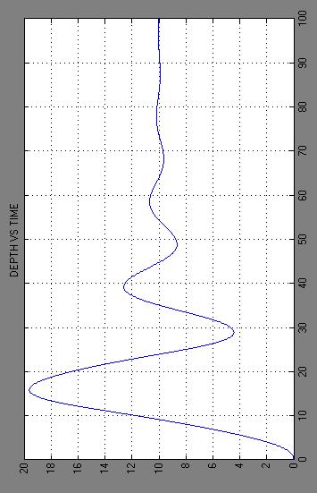
76 Linearization allows us to write W as: W = N dr/dt To give a numerical example we will let the parameters be: M = 50.0 N = 50.0 J = 0.5 I = 0.1 Theory shows that the borderline proportional gain KP for the auv is 6 and the borderline period TP is 14. The describing function for an ideal relay controller is: DF = [4 Qo] / [π Eo] At a limit cycle this is equal to the borderline proportional gain KP. Setting DF equal to KP gives: Eo = [4 Qo] / [π DF] = [4Qo] / [π KP] The saturation limit for the controller is 12. Substitution into the amplitude equation gives Eo equal to 2.5. An m code for the auv for the ideal relay controller case is given below. This is followed by a response generated by the code. As can be seen, it agrees with DF predictions.

77

78

79 PIPE FLOW SETUP To illustrate nonlinear phenomena, we will consider the task of controlling the temperature of air flowing down a pipe. The setup is shown on the next page. Relay controllers resemble the proportional controller. For the proportional controller case, the governing equations for the setup are: X dr/dt + Y R = H + D A dh/dt + B H = Z Q Q = KP E E = C - R where R is the temperature of the air at the heater, R is the temperature of the air at the sensor, C is the command temperature, E is the temperature error, Q is the control signal, H is the heat generated by the heater, D is a disturbance heat (plus or minus), X Y A B Z are process constants and KP is the controller gain. Note that R is what R was T seconds back in time: T is the time it takes for the air to travel down the pipe.

80

81 To give a numerical example we will let the parameters be: X = 0.25 Y = 1.0 A = 0.1 B = 1.0 Z = 1.0 T = 0.5 Theory shows that the borderline proportional gain KP for the setup is 1.5 and the borderline period TP is The describing function for an ideal relay controller is: DF = [4 Qo] / [π Eo] At a limit cycle this is equal to the borderline proportional gain KP. Setting DF equal to KP gives: Eo = [4 Qo] / [π DF] = [4Qo] / [π KP] The saturation limit for the controller is 5. Substitution into the amplitude equation gives Eo equal to 4.2. An m code for the setup for the ideal relay controller case is given below. This is followed by a response generated by the code. As can be seen, it agrees with DF predictions.

82

83