Is chaos possible in 1d? - yes - no - I don t know. What is the long term behavior for the following system if x(0) = π/2?

Transcription

1 Is chaos possible in 1d? - yes - no - I don t know What is the long term behavior for the following system if x(0) = π/2? In the insect outbreak problem, what kind of bifurcation occurs at fixed value of h (h>0)? (the sheet represents the fixed points) And at fixed value of r>0?

2 Summary of 1d flow The possible motions are (a) stay forever at a fixed point (b) go monotonically to a fixed point (c) go monotonically to +/- infinity Dependence in parameters renders 1d flow interesting!

3 Phase portraits and 3 types of bifurcations in 1d flows

4

5 Let s go to 2d where dynamics gets more interesting! We start simple with linear systems.

6 2d linear flows: linear systems A 2d linear system is a system of the form : matrix representation Where a, b, c and d are parameters. It is linear in the sense that if x 1 and x 2 are solutions, then is also a solution. The origin is always a fixed point.

7 2d linear flows : linear systems an example phase space Trajectories are tangent to the velocity field.

8 2d linear flows: another example Draw phase space for (a) a < -1 (b) a = - 1 (c) 0 < a < -1 (d) a = 0 (e) a > 0

9 2d linear flows: another example Stable node Star Stable node Line of fixed points Saddle point

10 2d linear flows: some terminology The y-axis is called here the stable manifold. It is the set of initial conditions such that x(t) -> x* as t -> infinity. Likewise, the unstable manifold is the set of initial conditions such that x(t) -> x* as t-> - infinity. What is the unstable manifold in this example? A fixed point is called * attracting: if all trajectories starting near x* approach it as t-> infinity * globally attracting: if for all initial conditions we have x-> x* as t-> infinity * Liapunov stable: if all trajectories starting close to x* stay close to x*. Can a fixed point be Liapunov stable but not attracting? * a fixed point that is Liapunov stable but not attracting is said neutrally stable. * a fixed point that is Liapunov stable AND attracting is said stable. * a fixed point which not Liapunov stable NOR attracting is said unstable. What about the stability of the fixed point in this 1d system?

11 IV. 2d linear flows : classification of linear systems Let us consider the general system: And look for solution of the form They are the analogous of the solutions we found for the example (v being the x or y axis), and must obey: This means that we need find eigenvalues and eigenvectors of the matrix A to find solution of this form. Typically, we have two independent eigenvalues and eigenvectors: If v1 and v2 are linearly independent, we can write any initial condition as unique solution of the 2d linear system is given by :. Therefore the

12 IV. 2d linear flows : example

13 IV. 2d linear flows : what about complex eigenvalues? α = 0 α<<0 Rem: for the solution to be real, we need c 1 v 1 and c 2 v 2 to be complex conjugates.

14 IV. 2d linear flows : what about degenerated cases? If both eigenvalues are equal, either the two eigenvectors are independent and we get a star: Or there is only one eigenvector. Imagine that the two eigenvectors (one slow, one fast) become closer and closer. This provides an idea of the structure of phase plane in the degenerate case:

15 IV. 2d linear flows : summary!!! Important!!!

16 V. 2d flows This equation can be seen as providing a velocity vector at each point x Dynamics is dictated by fixed points & closed orbits and their stability!

17 V. 2d flows : existence and uniqueness theorem An important implication of this theorem is that trajectories on phase space do not intersect.

18 V. 2d flows : linear stability analysis Let suppose that (x*,y*) is a fixed point, and consider small disturbances around it: The equations for those variable are and similarly for v:

19 V. 2d flows : linear stability analysis Let us rewrite those equations: We can rely on the theory of 2d linear system! Can we really always rely on the linear system?

20 V. 2d flows : linear stability analysis If Re(λ) 0 for both eigenvalues, the fixed point is said hyperbolic. In 1d systems, Re(λ) 0 is equivalent to f (x*) 0. In 2d systems, the linear stability analysis is valid for hyperbolic fixed points. In n dimensional systems, this result is still valid: STURDY FIXED POINTS = AWAY FROM IMAGINARY AXIS

21 V. 2d flows : Rabbits & sheep Lotka and Volterra proposed a model for the competition of two species for the same resource. Imagine - each species would grow to its carrying capacity in absence of the other (with a logistic growth). - when they encounter, trouble starts and they effectively decrease the growth rate of the other species. - the sheep decrease more the the growth rate of the rabbits than conversely.

22 V. 2d flows : Rabbits & sheep To analyze this system, let us first find the fixed points: Then for each point, do a linear stability analysis:

23 V. 2d flows : Rabbits & sheep To analyze this system, let us first

24 V. 2d flows : The principle of competitive exclusion separatrices

25 V. 2d flows : Conservative systems For a system a force depending only on position x (and not the velocity or explicit time dependence), It is possible to show that the energy is conserved and we can write the force in terms of a potential, Let s multiply by the velocity: We deduce that energy is conserved!

26 V. 2d flows : Conservative systems Attracting fixed points are not possible for conservative fixed points! Example: Homoclinic trajectories : they start and end at the same point.

27 V. 2d flows : Conservative systems

28 V. 2d flows : Reversible systems Many mechanical systems have a time-reversal symmetry. If you look at a movie of a pendulum backward, you will not notice.

29 V. 2d flows : Reversible systems

30 V. 2d flows : Index theory Index of a curve

31 V. 2d flows : Index theory

32 V. 2d flows : Index theory

33 V. 2d flows : Index theory

34 V. 2d flows : Index theory

35 V. 2d flows : Index theory The properties just seen ensure that we can define the index of a point as the index of any curve enclosing the fixed point and no other fixed points. What is the index of a stable node? Unstable node? Saddle?

36 V. 2d flows : Index theory

37 V. 2d flows : Index theory

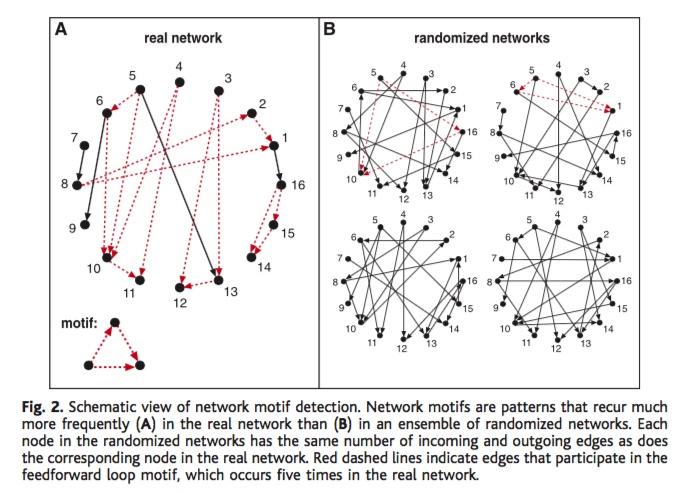
38 Transcription Translation Gene mrna Protein Decay Biology crash course for physicists:

39

40

41 Projects Goal : be able to represent a 2d phase portait with a computer program (preferably python), and to preform a bifurcation analysis/represent limit cycles. I am expecting an annotated code and an oral presentation (15-20 minutes). You should introduce the topic, the question addressed in the paper you chosen, present you code briefly and draw conclusion. How to give a good talk? howtogiveagoodtalk.pdf

42 Project #1: circadian rhythms Ordered phosphorylation governs oscillation of a three-protein circadian clock

43 Project #2: the repressilator synthetic biology

44 Project #3: The toggle switch Toggle switch A r nullcline c nullcline B r nullcline c nullcline cro concentration (nm) cro concentration (nm) ci concentration (nm) ci concentration (nm) Figure 7.11: Behaviour of the decision switch model. A. This phase portrait shows the bistable nature of the system. The nullclines intersect three times (boxes). The two steady states are found close to the axes; in each case the repressed protein is virtually absent. B. When RecA activity is included (by increasing δ r tenfold), the system becomes monostable all trajectories are attracted to the lytic (high-cro, low-ci) state. Parameter values: a =5min 1, b =50min 1, K 1 =1nM 2, K 2 =0.1 nm 1, K 3 =5nM 1, K 4 =0.5 nm 1, δ r =0.02 min 1 (0.2 in panel B), δ c =0.02 min 1. agradientofachemicalsignal calledamorphogen thatinduces differentiation into different cell types. The signal strength varies continuously over the tissuedomain,anddoesnotpersist indefinitely. In response, each cell makes a discrete decision (as to how to differentiate), and

45 Project #4: titration & oscillations in simple genetic circuits (a) (b) A I R I FIG. 1. (a) In the activator-titration circuit (ATC), the activator is constitutively produced at a constant rate and activates the expression of the inhibitor, which, in turn, titrates the activator into inactive complex. (b) In the repressor-titration circuit (RTC) the constitutively expressed inhibitor titrates the self-repressing repressor. FIG. 8. Bifurcation diagram of the RTC (a) and ATC (b) oscillators as a function of DNA unbinding rate (θ). All parameters, except θ, are the same as in Fig. 6. There are two bifurcation points (θ max,θ min ) and the amplitude of mrna oscillation is shown by the upper and lower branches. Physiological values of θ are to the right of the dashed vertical line.

46 Project #5: Neurons & excitable membranes Morris-Lescar model : Brian Ingall s book soma axon dendrites A Membrane Voltage (mv) mv 15 mv 13 mv +5 mv Potassium gating variable w Time (msec) 0 V nullcline 0.1 w nullcline Membrane Voltage V (mv)

47 Project #6: Microbiota & multistability Multi-stability and the origin of microbial community types

48 Project #7: Microbiota & prey-predator modeling Lotka-Volterra pariwise modeling fails to capture diverse pairwise microbial interactions panels_ajax_tab_tab=elife_article_author&panels_ajax_tab_trigger=article-info This project is about the fact that modeling microbial communities using Lotka-Volterra equations might fail to describe correctly the interactions between microbes as they are mediated via nutrient exchanges not explicitly modeled in LV equations (ie, the nutrient concentrations are not dynamical variables but implicitly described via constant interaction coefficients). Another possibility (project #8): We have seen the rabbit/sheep model based on Lotka-Volterra type of equations. These equations are used to model microbial communities. Our gut contains a great number of different microbial species. It is not yet clear under which conditions LV type of equations for many species possess a steady state. Since our gut microbial composition is rather stable, this question is relevant to construct realistic dynamical models of our gut flora. The feasibility of equilibria in large ecosystems: A primary but neglected concept in the complexitystability debate