ILC Group Annual Report 2018

Transcription

1 ILC Group Annual Report 28 D. SHEN

2 报告摘要 Letter 本报告主要汇总了智能与学习系统中心 (Center of Intelligent and Learning Systems) 在 28 年的研究内容 报告的主要内容包括研究组在本年度的相关数据 会议交流等学术活动 讨论组报告列表 研究生信息表 研究方向概述以及本年度发表论文集 本研究小组的主要研究方向为迭代学习控制 围绕这一方向, 研究组在本年度开展了一系列的研究, 在若干个方向上取得了重要突破 主要贡献如下 :. 在迭代学习控制综述方面, 发表了两篇综述, 分别是关于不完备信息环境下的迭代学习控制与随机迭代学习控制的设计与分析技术 ; 2. 针对批次变长度环境下连续时间非线性系统的采样迭代学习控制, 设计了原生 PD 型控制与含滑动平均的 PD 型控制, 分析了算法收敛性 ; 3. 针对参数化与非参数化连续时间非线性系统考虑批次变长度问题, 给出了新型的复合能量函数, 并证明了算法收敛性, 讨论了各种拓展情形 ; 4. 针对部分结构信息已知的连续时间非线性系统考虑批次变长度问题, 设计了时变参数与时不变参数可分情形与不可分情形下的两种混合算法 ; 5. 基于均匀量化器设计了含有编解码机制的量化迭代学习控制框架, 分别讨论了无限量化层级与有限量化层级的情形, 证明了跟踪误差渐进收敛至零 ; 6. 研究了异质高阶非线性模型所组成的多智能体系统含输出约束的分布式学习协同问题, 引入新型障碍函数来保证每个智能体的输出满足约束条件 本报告的最后一部分为本年度发表论文与在线发表论文的汇总

3 报告目录 Outline 研究组成员 2 研究方向概述 3 学术活动时间轴 4 讨论组内容简报 5 本年度论文列表

4 研究组成员 Members 曾春 女 26 年于北京化工大学获得学士学位现于北京化工大学攻读硕士学位获得 28 年国家奖学金研究方向 : 基于复合能量函数的变长度迭代学习控制已发表 SCI 论文 篇 刘辰 男 27 年于长安大学获得学士学位现于北京化工大学攻读硕士学位研究方向 : 多智能体迭代学习控制问题在投期刊论文 3 篇 瞿港归 男 28 年于华北电力大学保定校区获得学士学位现于北京化工大学攻读硕士学位研究方向 : 衰减信道下的迭代学习控制在投期刊论文 2 篇

5 霍妞 女 27 年于郑州航空工业管理学院获得学士学位现于北京化工大学攻读硕士学位研究方向 : 量化迭代学习控制 曾堃 男 26 年于北京航空航天大学获得学士学位现于北京化工大学攻读硕士学位研究方向 : 多智能体系统的迭代学习控制 OUR FAMILY

6 Group Alumni 王蓝菁 女 28 年于北京化工大学获得硕士学位研究生阶段发表 SCI 论文 篇 (Top 期刊 ) 硕士学位论文 批次变长度下连续系统的采样迭代学习控制 被评为校级优秀毕业论文. 章凡寿 男 28 年于北京化工大学获得硕士学位硕士学位论文 面向智能车与环境交互性的算法设计与分析 张超 男 28 年 2 月提前毕业于北京化工大学获得硕士学位研究生阶段发表 SCI 论文 4 篇获得 27 年国家奖学金硕士学位论文 基于编解码的量化迭代学习控制

7 2 研究方向概述 Research 本研究报告以迭代学习控制为核心研究方向 本年度主要的研究课题包括如下几 个方面 :. 批次变长度下的迭代学习控制 主要研究批次运行长度并非固定不变, 而是沿迭代轴方向随机变化情形的算法设计与分析问题 2. 量化迭代学习控制 在降低通信信道数据传输量及保证系统跟踪性能的矛盾要求下, 主要研究如何设计量化器以及相应的迭代学习控制算法的设计方案 3. 多智能体系统的迭代学习控制 针对各种类型的多智能体系统, 在不同的拓扑结构条件下, 如何设计分布式迭代学习控制算法并给出相应协同性能分析 4. 衰减信道下的迭代学习控制 主要研究网络化结构中传输信道存在随机衰减效应时对传输数据的影响, 以及如何进行算法设计与分析

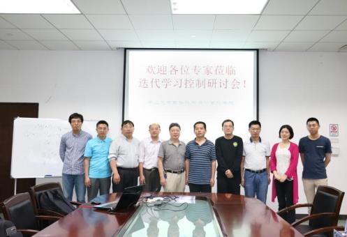
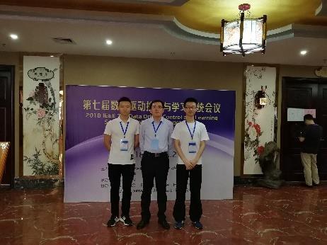
8 3 学术活动时间轴 Timeline 28. 在北京化工大学信息科学与技术学院新年学术报告会做学术报告 ( 沈栋 ) 28.3 中科院系统所随机系统建模与优化研讨会做学术报告 ( 沈栋 ) 28.5 受邀到访中山大学 华南理工大学进行学术交流 ( 沈栋 ) 28.5 参加在恩施举办的数据驱动控制与学习系统年会 ( 沈栋 张超 刘辰 )

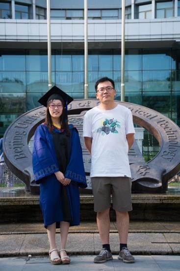
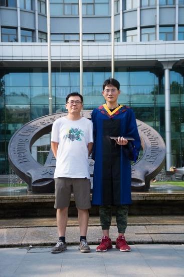
9 28.6 邀请宝马中国高级经理杨杰做关于汽车安全性的报告 ( 沈栋 ) 28.6 项目组王蓝菁 章凡寿获得硕士学位 28.7 受邀到访贵州大学进行学术交流 ( 沈栋 )

10 28.9 项目组曾春获得 28 年国家奖学金 28. 参加在临沂举办的自适应动态规划与强化学习研讨会 ( 沈栋 ) 28. 受邀参加由深科技与中国自动化学会联合举办的科创论坛并做报告 ( 沈栋 )

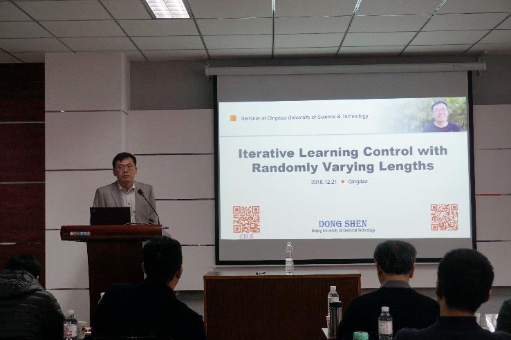
11 28.2 受邀到访西安电子科技大学进行学术交流 ( 沈栋 ) 28.2 邀请广西科技大学戴喜生教授 中山大学李晓东教授 华南理工大学田森平教授到访 28.2 参加在青岛举办的大数据环境下智能学习控制理论研讨会 ( 沈栋 )

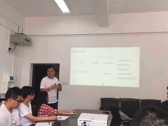
12 4 讨论组内容简报 Seminar 本年度讨论组内容不是针对文章展开, 而是围绕学习迭代学习控制的基本概念与常用技巧等展开, 主要报告内容围绕下述手稿展开, 具体分工章节不再罗列

13 5 本年度论文列表 Publications Journal Papers. Lanjing Wang, Xuefang Li, Dong Shen*. Sampled-data Iterative Learning Control for Continuous-time Nonlinear Systems with Iteration-Varying Lengths. International Journal of Robust and Nonlinear Control, vol. 28, no. 8, pp , Jian Han, Dong Shen*, Chiang-Ju Chien. Terminal Iterative Learning Control for Discrete-Time Nonlinear Systems Based on Neural Networks. Journal of the Franklin Institute, vol. 355, no. 8, pp , Dong Shen*. Data-Driven Learning Control for Stochastic Nonlinear Systems: Multiple Communication Constraints and Limited Storage. IEEE Transactions on Neural Networks and Learning Systems, vol. 29, no. 6, pp , Dong Shen*, Chao Zhang, Yun Xu. Intermittent and Successive ILC for Stochastic Nonlinear Systems with Random Data Dropouts. Asian Journal of Control, vol. 2, no. 3, pp. 2-4, Dong Shen*. Iterative Learning Control with Incomplete Information: A Survey. IEEE/CAA Journal of Automatica Sinica, vol. 5, no. 5, pp , Yanqiong Jin, Dong Shen*. Iterative Learning Control for Nonlinear Systems with Data Dropouts at Both Measurement and Actuator Sides. Asian Journal of Control, vol. 2, no. 4, pp , Dong Shen*, Jian-Xin Xu. Distributed Learning Consensus for Heterogenous High-Order Nonlinear Multi-Agent Systems with Output Constraints. Automatica, vol. 97, no , Dong Shen*. A Technical Overview of Recent Progresses on Stochastic Iterative Learning Control. Unmanned Systems, vol. 6, no. 3, pp , Chao Zhang, Dong Shen*. Zero-Error Convergence of Iterative Learning Control Based on Uniform Quantisation with Encoding and Decoding Mechanism. IET Control Theory & Applications, vol. 2, no. 4, pp , 28.. Chun Zeng, Dong Shen*, JinRong Wang. Adaptive Learning Tracking for Uncertain Systems with Partial Structure Information and Varying Trial Lengths. Journal of the Franklin Institute, vol. 355, no. 5, pp , 28.. Zhijiang Lou, Dong Shen, Youqing Wang*. Two-Step Principal Component Analysis for Dynamic Processes Monitoring. Canadian Journal of Chemical Engineering, vol. 96, no., pp. 6-7, JinRong Wang*, Zijian Luo, Dong Shen. Iterative Learning Control for Linear Delay Systems with Deterministic and Random Impulses. Journal of the Franklin Institute, vol. 355, no. 5, pp , Saurab Verma, Dong Shen, Jian-Xin Xu*. Motion Control of Robotic Fish under

14 Dynamic Environmental Conditions using Adaptive Control Approach. IEEE Journal of Oceanic Engineering, vol. 43, no. 2, pp , Dahui Luo JinRong Wang, Dong Shen. Learning Formation Control for Fractional-Order Multi-Agent Systems. Mathematical Methods in the Applied Sciences, vol. 4, no. 3, pp , Shengda Liu, JinRong Wang*, Dong Shen, Donal O'Regan. Iterative Learning Control for Noninstantaneous Impulsive Fractional Systems with Randomly Varying Trial Lengths. International Journal of Robust and Nonlinear Control, vol. 28, no. 8, pp , Xiaowen Wang, JinRong Wang*, Dong Shen, Yong Zhou. Convergence Analysis for Iterative Learning Control of Conformable Fractional Differential Equations. Mathematical Methods in the Applied Sciences, vol. 4, no. 7, pp , Chengbin Liang, Jinrong Wang*, Dong Shen. ILC for Linear Discrete Delay Systems via Discrete Matrix Delayed Exponential Function Approach. Journal of Difference Equation and Applications, vo. 24, no., pp , 28. Online Journal Papers 8. Dong Shen*, Jian-Xin Xu. Adaptive Learning Control for Nonlinear Systems with Randomly Varying Iteration Lengths. IEEE Transactions on Neural Networks and Learning Systems. 9. Dong Shen*, Jian-Xin Xu. Robust Learning Control for Nonlinear Systems with Nonparametric Uncertainties and Non-uniform Trial Lengths. International Journal of Robust and Nonlinear Control. 2. Shengda Liu, JinRong Wang*, Dong Shen, D. O'Regan. Iterative Learning Control for Differential Inclusions of Parabolic Type with Noninstantaneous Impulses. Applied Mathematics and Computation. Conference Papers 2. Chen Liu, Dong Shen*. Iterative Learning Consensus for Discrete-time Multi- Agent Systems with Measurement Saturation and Random Noises. The 28 IEEE 7th Data Driven Control and Learning Systems Conference, Enshi, China, May 25-27, 28, pp Chao Zhang, Dong Shen*. Finite-Level Quantized Iterative Learning Control by Encoding- Decoding Mechanisms. The 28 IEEE 7th Data Driven Control and Learning Systems Conference, Enshi, China, May 25-27, 28, pp (Best Paper Award Finalist)

15 Received: 24 March 27 Revised: 8 November 27 Accepted: 22 January 28 DOI:.2/rnc.466 RESEARCH ARTICLE Sampled-data iterative learning control for continuous-time nonlinear systems with iteration-varying lengths Lanjing Wang Xuefang Li 2 Dong Shen College of Information Science and Technology, Beijing University of Chemical Technology, Beijing, China 2 Department of Electrical and Electronic Engineering, Imperial College London, London, UK Correspondence Dong Shen, College of Information Science and Technology, Beijing University of Chemical Technology, Beijing 29, China. shendong@mail.buct.edu.cn Funding information National Natural Science Foundation of China, Grant/Award Number: and 63485; Beijing Natural Science Foundation, Grant/Award Number: 4524 Summary In this work, sampled-data iterative learning control (ILC) method is extended to a class of continuous-time nonlinear systems with iteration-varying trial lengths. In order to propose a unified ILC algorithm, the tracking errors will be redefined when the trial length is shorter or longer than the desired one. Based on the modified tracking errors, 2 sampled-data ILC schemes are proposed to handle the randomly varying trial lengths. Sufficient conditions are derived rigorously to guarantee the convergence of the nonlinear system at each sampling instant. To verify the effectiveness of the proposed ILC laws, simulations for a nonlinear system are performed. The simulation results show that if the sampling period is set to be small enough, the convergence of the learning algorithms can be achieved as the iteration number increases. KEYWORDS initial state condition, iteration learning control, iteration-varying lengths, iteratively moving average operator, relative degree, sampled-data INTRODUCTION Iterative learning control (ILC) is an effective control strategy for systems operating on a finite interval repeatedly. It can be applied to improve the control performance by learning from the previous control experience. That is, the control and tracking information of previous iterations can be fully employed to generate the control signal for the current iteration. In this case, the tracking performance can be gradually improved as the iteration number increases. This ILC was first proposed in 984 by Arimoto et al for precise robot tracking and now has been fruitful in both the underlying theory and experimental applications in other works. 2-4 Over the past 3 decades, ILC has been extensively investigated in various issues including robust design, 5 distributed algorithms, 6,7 monotonic convergence, 8 and networked configuration. 9, Typical applications of ILC can be found in various robots,2 and industrial devices. 3,4 In classic ILC, it requires that every execution (trial, iteration, pass) must be completed in a fixed time duration. However, in many practical control systems, this requirement may not hold due to the limitations of control objects, system constraints, or safety problems. For instance, when stroke patients do the rehabilitation via functional electrical stimulation, sometimes the process has to be terminated midway if the patients do not feel well. 5-7 However, this incomplete treatment information is also very helpful to the upcoming treatments. From ILC point of view, this example forms an ILC problem with iteration-varying trial lengths. Another example is the gait problems of humanoid robots discussed in the works of Longman and Mombaur, 8 in which the walking motion is divided into phases defined by foot strike Int J Robust Nonlinear Control. 28;28: wileyonlinelibrary.com/journal/rnc Copyright 28 John Wiley &Sons,Ltd. 373

16 374 WANG ET AL. times and the durations of phases are different from cycle to cycle during the learning process. This also will lead to a nonuniform trial length problem. Furthermore, system input/output constraints will also imply nonrepeatable trial lengths in ILC design, such as the lab-scale gantry crane system given in the work of Guth et al. 9 When the output constraints are violated, the load is wound up and the trial has to be terminated, which makes the trial lengths different from trial to trial. Generally, nonuniform trial length problem may often happen when applying ILC to practical applications in consideration of operation safety. Hence, it is important to investigate ILC for systems with iteration-varying trial lengths. In the past few years, several works related to ILC with variable trial lengths have been published For instance, Li et al 2-23 introduce a newly defined stochastic variable and an iteration-average operator into ILC algorithm to deal with the randomly varying trial lengths of both discrete-time linear and continuous-time nonlinear systems, where the convergence of the tracking error is derived in the sense of mathematical expectation. Motivated by the works of Li et al, 2-23 Shen et al 24 extend ILC with variable pass lengths to a class of discrete-time nonlinear systems. Furthermore, Shen et al 25,26 derive the convergence of a P-type updating law with nonuniform trial lengths in the sense of almost sure and mean square. Additionally, Seel et al 2 mainly focus on the monotonic convergence property of ILC with variable pass lengths, where the proposed ILC law has been implemented in functional electrical stimulation based treatment for stroke patients in their other works. 6,7 Shi et al 27 further extend the concept of ILC with iteration-varying trial lengths to a class of stochastic systems. Moreover, Liu and Liu 28 discuss ILC with randomly varying trial lengths under the framework of Lyapunov theory. However, it is worthy to mention that most existing literature concentrate on discrete-time or continuous-time systems and major results are derived for linear systems. Taking the practical systems and computer-aided design methodology into account, it is natural and meaningful to consider the sampled-data control and investigate how sampled-data ILC with nonuniform trial lengths works. However, to our best knowledge, no paper has been reported on this topic. In literature, there are many works focusing on ILC design for sampled-data systems since most of the control plants in practice are continuous-time systems, but the digital implementation is discrete-time. Nevertheless, these works only consider the sampled-data ILC with identical trial length. Note that the uniform trial length case can be regarded as a special case of the uniform trial lengths problem, thus the results derived in this paper would include the existing results on sampled-data ILC as special cases. In other words, our results extend the application range of sampled-data ILC. In this paper, we aim at sampled-data ILC design for continuous-time nonlinear systems with randomly varying trial lengths. To deal with the iteration-varying trial lengths, 2 sampled-data ILC schemes are proposed based on the modified tracking errors that have been redefined when the trial length is shorter or longer than the desired one. Sufficient conditions are derived rigorously to guarantee the convergence of the nonlinear system at each sampling instant. To verify the effectiveness of the proposed ILC laws, simulations for a nonlinear system are also performed. The simulation results show that if the sampling period is set to be small enough, the convergence of the learning algorithms can be achieved as the iteration number increases. The main contributions of this work are summarized as follows. We provide the first result on sampled-data ILC for continuous-time nonlinear systems with iteration-varying lengths. This work fulfills the gap for completing the explorations on ILC under iteration-varying lengths. We present an in-depth convergence analysis of the generic and iteration-moving-averaged PD-type ILC update laws. The sufficient conditions for asymptotical convergence are derived rigorously by using contraction mapping method. We consider the general relative degree for nonlinear systems and its effect on the convergence. The impact of initial state deviations on the final tracking performance is also discussed. This paper is organized as follows. Section 2 presents the descriptions of sampled-data ILC methodology to a class of nonlinear systems with randomly varying trial lengths and higher relative degree. In Section 3, two ILC algorithms are proposed associated with their convergence analysis for the identical initial condition case. In Section 4, the influence of varying initial states is discussed for the proposed ILC algorithms. Furthermore, an illustrative example is given in Section 5. Notation. denotes the Euclidean norm. E( ) denotes the mathematical expectation. θ(i) λ = sup i Ω α λi E θ(i) indicates the λ norm of a vector θ(i),whereλ>,α >, and Ω is a finite set of i.

17 WANG ET AL PROBLEM FORMULATION 2. System description Consider the following continuous-time nonlinear system: ẋ k (t) =f (x k (t)) + B (x k (t)) u k (t) y k (t) =g (x k (t)), () where k =,, denotes the iteration index, t [, T k ] denotes the time index, and T k is the actual trial length of the kth iteration. Moreover, x k (t) R n, u k (t) R p,andy k (t) R q are the state, the control input, and the output of system (), respectively. The nonlinear functions f( ) R n, B( ) R n p,andg( ) = [g ( ), g 2 ( ),, g q ( )] T R q are smooth in their domain of definition. Let h be the sampling period of the sampler and n k =[T k h] be the actual sampling number in the kth iteration. The notation [ι] means the largest integer less or equal to ι. Furthermore, the desired trajectory is denoted by y d (t) and assumed to be realizable, where t [, T d ], T d is the desired length of each iteration and n d =[T d h] is the largest number of desired sampling instants. The control input is derived from the ILC law that is designed by using the sampling signal. In order to generate a continuous control input, the zero-order holder device is adopted. Then, the continuous-time control signal is taken piecewise constant between the sampling instants u k (t) =u k (ih), (2) where t [ih, ih + h), i n k. The control objective in this paper is to design a sampled-data ILC law u k (ih) such that the output error at each sampling instant satisfies lim k y d (ih) y k (ih) =, i n k. To describe the input-output causal relationship of system (), we need the derivative notations that are defined as L f g(x) = g(x) x f(x) and ( L j f g(x) =L f L j f ) g(x) = L b L f g(x) = L f g(x) b(x) x with L g(x) =g(x), where the superscript means no derivative operation. f Definition. (See the work of Sun and Wang 3 ) The continuous-time nonlinear system () has extended relative degree {β,β 2,,β q } for x(t) and the following conditions hold:. 2. ih ih+h ih+h ih where j β m 2; 3. the q p matrix is of full-column rank. [ ih+h t ih ih t β ih ih+h t ih ih t [ β q ih ( L j f x ) g(x) f(x) L br g m (x(t )) dt =, r p, m q; ih t L b L β f L b L β q f ih t j L br L j f g m(x(t j+ ))dt j+ dt =, ( g x(tβ ) ),, L bp L β ( g f x(tβ ) ) dt β dt ( g q x(tβq ) ),, L bp L β q ( g f q x(tβq ) ). dt βq dt

18 376 WANG ET AL. From system () and Definition, we can derive that the mth component of system output at the sampling instant ih+h of thekth iteration is evaluated as hβ m y m,k (ih + h) =y m,k (ih)+hl f g m (x k (ih)) + + (β m )! Lβ m g f m (x k (ih)) ih+h t t βm + L ih ih β m f g ( ( )) m xk tβm dtβm dt (3) ih ih+h t t βm [ + L b L β ( ( )) m g f m xk tβm,, Lbp L β ( ( )) ] m g f m xk tβm dt βm dt u k (ih). ih ih ih It indicates that the output y m,k (ih + h) is obtained from the control input u k (ih).thus,{u k (ih), y m,k (ih + h), m q} is a pair of dynamically related cause and effect. Assumptions are as follows. Assumption. For any realizable reference trajectory y d (t), there exist a suitable initial state x d () and unique input u d (t) R p such that ẋ d (t) =f (x d (t)) + B (x d (t)) u d (t) y d (t) =g (x d (t)), (4) where t [, T d ] and u d (t) is uniformly bounded for all t [, T d ]. Assumption 2. For each fixed x k (), the mappings S (a mapping from (x k (), u k (t), t [, T k ]) to (x k (t), t [, T k ])) and O (a mapping from (x k (), u k (t), t [, T k ]) to (y k (t), t [, T k ]))areonetoone. Assumption 3. The system has extended relative degree {β,β 2,,β q } for x(t), t [, T d ]. Assumption 4. The functions f( ), g( ), B( ), L j f g m( ),andl br L β m g f m ( ), j β m, m q, r p are globally Lipishitz in x on [, T d ]. The Lipishitz constants are denoted by l f, l g, l B, l Lf,andL bf, respectively. Remark. Assumption presents the realizability of the reference trajectory, which is widely used in the existing literature for nonlinear systems. Indeed, this assumption can be guaranteed by Assumption 2, while Assumption 2 further implies the existence and uniqueness of the solution to system (). Assumption 3 describes the extend relative degree, where the latter is defined above. Assumption 4 is imposed to limit the nonlinearities so that the Gronwall inequality and contraction mapping method can be applied to derive the strict convergence analysis. Assumption 5. The initial state conditions are identical in each iteration, ie, x k () =x d (), k. Assumption 6. The initial states for any iteration are bounded, ie, x d () x k () ε,whereε is a positive constant. Remark 2. Assumption 5 is imposed to ensure perfect tracking performance. However, in many practical applications, the identical initial states in each iteration cannot hold, because the value of initial state x k () may not be reset accurately in each iteration. Thus, Assumption 6 is given to relax such assumption to the case that the initial state deviations are bounded. Clearly, Assumption 6 holds generally for most practical systems. Assumptions 5 and 6 will be addressed in Sections 3 and 4, respectively. 2.2 Problem description In this paper, we consider the continuous-time nonlinear system with iteration-varying lengths. In order to improve the performance by ILC, it is necessary to suitably address the randomness of the actual trial length T k in each iteration. Without loss of generality, assume that there exist a minimal trial length T min and a maximal trial length T max,andthe actual trial length in each iteration varies among [T min, T max ]. Besides, the desired trial length T d satisfies the condition T min T d T max.

19 WANG ET AL. 377 Let T k be a stochastic variable and the probability of the output occurrence at time t be p(t), then the probability distribution function of T k is, t [, T min ) P(T k t) = p(t), t [T min, T max ], t (T max, + ], where p(t). Besides, the output at any time t < t is available in an iteration if the output at time t is available in the same iteration. Similar to the work of Liu and Liu, 28 we can define the general form of this probability distribution without prior information {, t [, T min ) p(t) = p max + T max ς(τ)dτ, t [T t min, T max ] T max ς(τ)dτ = p max, T min where ς(τ) is a probability density function, p max > is the probability of the event that the trial length is T max,andthus the probability p(t) satisfies the condition <p max p(t). Furthermore, compared with the Gaussian probability distribution in the work of Shi et al, 27 p(t) is of no prior form in this work. As a result, the formulation of randomly varying lengths in the aforementioned work 27 can be seen as a special case of the formulation in this paper. Obviously, there are 2 cases for sampling numbers to be addressed, ie, n k < n d and n k n d. For the former case, the kth iteration would end before the desired trial length is achieved, and the outputs on the interval (n k, n d ] are missing, which are not available for updating. For the latter case, the kth iteration will still run up to the time instant n k instead of stopping at n d. It is observed that the data after the time instant n d are redundant and useless for learning. Without loss of generality, we could simply let the latter case be n k = n d. Then, let (ih n k h), i [, n d ] be a stochastic variable taking binary values and. Here, (ih n k h)=denotes the event that the control process can last beyond the sampling time instant ih, which occurs with a probability of p(ih),where < p(ih) <, whereas (ih n k h)=denotes the event that the control process cannot continue to the sampling time instant ih, which occurs with a probability of p(ih). It is apparent that (ih n k h) satisfies the Bernoulli distribution, thus we can derive the expectation E{(ih n k h)} = p(ih)+ ( p(ih)) = p(ih). Therefore, we can define a modified tracking error as follows: { e k (ih) = e k (ih) i n k (5) (n k + ) i n d, where e k (ih) y d (ih) y k (ih) is the original tracking error. Then, (5) could be reformulated as e k (ih) =(ih n kh)e k (ih). (6) Lemma. (See the work of Shen et al 24 ) Let ξ be a Bernoulli binary random variable with P(ξ = ) = ξ and P(ξ = ) = ξ. If there exists a positive matrix Ψ, the equality E I ξψ = I ξψ holds if and only if one of the following conditions is satisfied: (i) ξ = or ξ = ; (ii) < ξ <; and (iii) < Ψ I. 3 SAMPLED-DATA ILC DESIGN AND CONVERGENCE ANALYSIS Two ILC laws with the modified tracking error are introduced in this section, and convergence analyses are addressed. 3. Generic proportional-derivative (PD) type ILC scheme The generic PD-type ILC is given by u k+ (ih) =u k (ih)+k P e k ((i + )h) + K ( D e k ((i + )h) e k (ih)), (7) where i n d, and K P R p q and K D R p q are proportional and derivative learning gains, respectively. These gains will be defined in the following.

20 378 WANG ET AL. Theorem. Consider the continuous-time nonlinear system () with Assumptions to 5. Let the PD-type ILC law (7) be applied with learning gains K P and K D satisfying sup k where N k (ih) =(K P + K D )((i + )h n k h) and [ ih+h t ih ih t β ih ψ k (ih) = ih+h t ih ih t [ β q ih supe I N k (ih)ψ k (ih) σ<, (8) i L b L β f L b L β q f ( ( )) g x tβ,, Lbp L β ( ( )) g f x tβ dtβ dt ( ( )) g q x tβq,, Lbp L β q ( ( )). g f q x tβq dtβq dt If the sampling period h is chosen small enough, then the system output y k (ih) converges to y d (ih) for all i [, n d ] as k. Proof. Define δu k ( ) = u d ( ) u k ( ) and δx k ( ) = x d ( ) x k ( ). It follows from (6) and (7) that δu k+ (ih) =δu k (ih) K P e k ((i + )h) K ( D e k ((i + )h) e k (ih)) = δu k (ih) (K P + K D )e k ((i + )h) + K De k (ih) = δu k (ih) N k (ih)e k ((i + )h) + M k (ih)e k (ih), where N k (ih) =(K P + K D )((i + )h n k h) and M k (ih) =K D (ih n k h). From (3), the mth component of tracking error at the sampling time instant (i + )h can be expressed as where e m,k ((i + )h) = y m,d ((i + )h) y m,k ((i + )h) = e m,k (ih)+υ m,k (ih)+ω m,k (ih)+ψ m,k (ih)δu k (ih), e m,k (ih) =g m (x d (ih)) g m (x k (ih)), υ m,k (ih) =h [ L f g m (x d (ih)) L f g m (x k (ih)) ] + + [ hβ m (β m )! L β m f ] g m (x d (ih)) L β m g f m (x k (ih)) ih+h t t βm [ ω m,k (ih) = L ih ih β m f g ( m xd (t βm ) ) L β m f g ( m xk (t βm ) )] dt βm dt ih ih+h t t βm [ + L ih ih b L β ( m g f m xd (t βm ) ),, L bp L β ( m g f m xd (t βm ) )] ih [ L b L β ( m g f m xk (t βm ) ),, L bp L β ( m g f m xk (t βm ) )] dt βm dt u d (ih) ih+h t t βm [ ψ m,k (ih) = L ih ih b L β ( m g f m xk (t βm ) ),, L bp L β ( m g f m xk (t βm ) )] dt βm dt. ih The tracking error at time instant (i + )h can be written as where Substituting () into (9) yields e k ((i + )h) = e k (ih)+υ k (ih)+ω k (ih)+ψ k (ih)δu k (ih), () e k (ih) = [ e,k (ih),, e q,k (ih) ] T, υ k (ih) = [ υ,k (ih),,υ q,k (ih) ] T, ω k (ih) = [ ω,k (ih),,ω q,k (ih) ] T, [ ] T. ψ k (ih) = ψ T,k (ih),, ψt q,k (ih) δu k+ (ih) =(I N k (ih)ψ k (ih)) δu k (ih)+(m k (ih) N k (ih)) e k (ih) N k (ih) (υ k (ih)+ω k (ih)). (2) Taking norms to both sides of (2) and applying the Lipschitz condition in Assumption 4, we have δu k+ (ih) I N k (ih)ψ k (ih) δu k (ih) + l g γ m δx k (ih) + γ n ( υ k (ih) + ω k (ih) ) (3) (9) ()

21 WANG ET AL. 379 and υ k (ih) γ δx k (ih), ω k (ih) γ 2 ih+h t ih ih t β ih δx k(t β ) dt β dt ih+h ih t ih t β q ih δx k(t βq ) dt βq dt { } where γ = max h m q + + hβ m l! (β m )! Lf, γ 2 = l Lf + pl bf ρ ud, ρ ud = sup i nk u d(ih), γ m is the norm bound for (M k (ih) N k (ih)) and γ n is the norm bound for N k (ih). From () and (4), we can obtain t t δx k (t) = [f (x d (τ)) f (x k (τ))] dτ + [B (x d (τ)) u d (τ) B(x k (τ)) u k (τ)] dτ, (4) ih where t [ih, ih + h]. Then, taking the norms and applying Bellman-Gronwall's lemma to (4) results in that ih, t δx k (t) δx k (ih) e γ3(t ih) + e γ3(t s) γ B δu k (s) ds, δx k (t) γ 4 δx k (ih) + γ 5 δu k (ih), ih (5) where γ 3 = l f + l B ρ ud, γ 4 = e γ3h, γ 5 = γ B(γ 4 ),andγ γ B is the norm bound for B(x k (t)). Moreover, we can obtain 3 δx k (ih) γ 4 δx k ((i )h) + γ 5 δu k ((i )h). (6) According to Assumption 5, ie, x k () =x d () for all k,ithas Then, (3) can be rewritten as i δx k (ih) γ 5 γ i j δu 4 k ( jh). (7) j= δu k+ (ih) ρ k (ih) δu k (ih) + γ 6 δx k (ih), (8) i δu k+ (ih) ρ k (ih) δu k (ih) + γ 5 γ 6 γ i j δu 4 k ( jh), (9) { } where ρ k (ih) =ρ k (ih)+γ 2 γ 5 γ h γ n, ρ k (ih) = I N k (ih)ψ k (ih), γ h = max h β,, hβq,andγ β! β q! 6 =(γ +γ 2 γ 4 γ h )γ n +l g γ m. Clearly, sufficiently small sampling period h yields arbitrarily small γ h. Furthermore, taking mathematical expectation to both sides of (9), we have ( ) i E δu k+ (ih) E ( ρ k (ih) δu k (ih) ) + E γ 5 γ 6 γ i j δu 4 k ( jh) j= j= i E ( ρ k (ih)) E δu k (ih) + γ 5 γ 6 γ i j E δu 4 k ( jh), where E( ρ k (ih)) = E(ρ k (ih)) + γ 2 γ 5 γ h γ n and E(ρ k )=E I N k (ih)ψ k (ih). Multiplying both sides of (2) with α λi and taking supremum for all time instants i yields supα λi E δu k+ (ih) supe( ρ k )supα λi E δu k (ih) + γ 5 γ 6 sup i i i i j= i α λi γ i j j= (2) 4 E δu k ( jh). (2)

22 38 WANG ET AL. Let α>γ 4, then we can drive that sup i i α λi γ i j j= 4 E δu k ( jh) sup i i α λi j= i α sup i j= α i j E δu k ( jh) ( sup j i α δu k (ih) λ sup i η d δu k (ih) λ, ( α λj E δu k ( jh) ) α (λ )(i j) ) α (λ )(i j) j= (22) where η d = α (λ )n d. α λ α Substituting (22) into (2) implies that δu k+ (ih) λ sup E ( ρ k (ih)) δu k (ih) λ + γ 5 γ 6 η d δu k (ih) λ. (23) i Let and we have μ = sup k sup E ( ρ k (ih)) i κ = γ 5 γ 6, δu k+ (ih) λ (μ + κη d ) δu k (ih) λ. (24) Let α>max{,γ 4 }, then it is possible to choose a sufficiently small sampling period h and a sufficiently large λ such that κη d = κ α (λ )n d (25) α λ α is arbitrarily small. Thus, if (8) holds i, there exist sufficiently small h and sufficiently large λ such that μ + κη d ζ<. Then, it is guaranteed that lim δu k(ih) λ =, i. k According to the finiteness of i, it follows lim E δu k(ih) =, i. k Noticing δu k (ih), we obtain lim δu k(ih) =, i. k Then, it is easy to conclude the results lim k δx k (ih) =andlim k e k (ih) =, i. This completes the proof. Theorem presents an explicit sufficient condition guaranteeing the asymptotical convergence of the tracking errors at sampling time instants for the generic PD-type sampled-data ILC for nonlinear systems with iteration-varying lengths. The sufficient condition (8) indicates that gains of both P-part and D-part of the update law would affect the convergence. It is worthwhile to mention that the proposed sampled-data ILC is able to work well without an accurate system model. The learning gains can be determined by some approximations while the sampling period is sufficiently small. Noting that mathematical expectation is involved in the convergence condition, we can remove this operator by strengthening the design of learning gains as in the following corollary. Corollary. Consider the continuous-time nonlinear system () and Assumptions to 5. Let the PD-type ILC law (7) be applied with learning gains K P and K D satisfying < (K P + K D )ψ k (ih) < I, sup k sup I (K P + K D )p ((i + )h) ψ k (ih) <. i (26)

23 WANG ET AL. 38 Then, the system output y k (ih) converges to y d (ih) for all i [, n d ] as k if the sampling period h is chosen small enough. Proof. Applying the results in Lemma to condition (8) in Theorem, we can complete the proof of this corollary. Remark 3. In Theorem, we depict a qualitative expression of the sampling period h to guarantee the asymptotical convergence that the sampling period should be small enough. One may interest in how is the explicit range of the sampling period. Indeed, it is difficult to determine the period because of the nonlinearities in the system and controller. Generally, it is seen from (24) that the sampling period should ensure that γ 2 γ 5 γ h γ n + κη d < σ. Sincewe can always select sufficiently large α to make κη d arbitrarily small, we should still ensure γ 2 γ 5 γ h γ n < σ.inpractical applications, we find that a small sampling period implies a better control performance. From this point of view, it is suggested to select the possible smallest sampling period to guarantee the convergence condition and improve the actual tracking performance in the meantime. 3.2 The modified ILC scheme An iteratively moving average operator is used in this section to solve the problem of sampled-data ILC for nonlinear systems with iteration-varying lengths. Compared with the iteration-averaging techniques used in the works of Li et al 22,23 and Shi et al, 27 the iteratively moving average operator in this paper only use the information of several previous trials to compensate the absent tracking information. The inherent reason lies in that the data from early iterations may be useless for current input updating, while the information of adjacent iterations would be helpful in correcting the input signals. Definition 2. (See the work of Li et al 23 ) For a sequence f k r ( ), f k r+ ( ),, f k ( ) with r, an iteratively moving average operator is defined as {f k ( )} r f k j ( ), (27) r + j= where r + is the size of the moving window. As a special case, the iteratively moving average operator of the mth component of the vector sequence is represented as { f m k ( )} r f m ( ). (28) r + k j Design an iteratively moving average operator-based PD-type ILC law as follows: u k+ (ih) = {u k (ih)} + K P { e k ((i + )h)} + K D { e k ((i + )h) e k (ih)}, (29) where K R p q and K P D Rp q are proportional and derivative learning gains, respectively. These gains will be determined in the following. In addition, we assume that u (ih) =u 2 (ih) = = u z (ih) = without loss of any generality. Theorem 2. Consider the continuous-time nonlinear system () with Assumptions to 5. Let the PD-type ILC law (29) be applied with learning gains K P and K D satisfying r θ w σ<, (3) w= where θ w r + sup sup E I N k w (ih)ψ k w (ih) k i and N k w (ih) =(K P + K D )((i + )h n k wh). If the sampling period h is chosen small enough, then the system output y k (ih) converges to y d (ih) for all i [, n d ] as k. Proof. Substituting (6), (27) into (29) yields to u k+ (ih) = r u k w (ih)+ r N k w (ih)e k w ((i + )h) r M k w (ih)e k w (ih), (3) r + r + r + w= w= j= w=

24 382 WANG ET AL. where M k w (ih) =K D (ih n k wh) and N k w (ih) =(K P + K D )((i + )h n k wh). Then, it follows that r ( δu k+ (ih) = I Nk w (ih)ψ k w (ih) ) δu k w (ih) r + w= r ( + Mk w (ih) N k w (ih) ) e k w (ih) r + w= r r + N k w (ih) (υ k w (ih)+ω k w (ih)). w= (32) Taking norms to both sides of (32) and applying the Lipschitz condition in Assumption 4 yields that r δu k+ (ih) ( I Nk w (ih)ψ k w (ih) ) w= r + δu k w (ih) + r r + l gγ m δx k w (ih) w= + r r + γ n ( υ k w (ih) + ω k w (ih) ), w= where γ m is the norm bound for (M k w (ih) N k w (ih)) and γ n is the norm bound for N k w (ih). Then, from (7), we have i δx k w (ih) γ 5 γ i j δu 4 k w ( jh), (34) j= υ k w (ih) + ω k w (ih) (γ + γ 2 γ 4 γ h ) δx k w (ih) + γ 2 γ 5 γ h δu k w (ih). (35) Combing (33), (34) and (35), we can obtain δu k+ (ih) i r ρ r + k w (ih) δu r k w(ih) + γ 5 γ 7 γ i j δu r + 4 k w ( jh), (36) w= w=j= where ρ (ih) =ρ k w k w (ih)+γ 2 γ 5 γ h γ n, ρ k w (ih) = I N k w (ih)ψ k w (ih),andγ 7 =(γ + γ 2 γ 4 γ h )γ n + l g γ m. Taking mathematical expectation to both sides of (36), we can conclude that ( ) ( ) i r E δu k+ (ih) E ρ r + k w (ih) δu r k w(ih) + E γ 5 γ 7 γ i j δu r + 4 k w ( jh) w= w= w=j= r E ( i ρ r + k w (ih)) r E δu k w (ih) + γ 5 γ 7 γ i j E δu r + 4 k w ( jh), w=j= where E( ρ (ih)) = E(ρ k w k w (ih)) + γ 2 γ 5 γ h γ n and E(ρ k w (ih)) = E I N k w (ih)ψ k w (ih). Multiplying both sides of (37) with α λi and taking supremum for all time instants i,wehave sup α λi E δu k+ (ih) r supe ( ρ i r + k w (ih)) sup α λi E δu k w (ih) w= i i i r +γ 5 γ 7 r + sup α λi γ i j E δu 4 k w ( jh) i and sup i α λi w= w=j= w=j= i r r γ i j E δu 4 k w ( jh) η d δu k w (ih) λ. (39) Thus, (38) can be rewritten as δu k+ (ih) λ r sup E ( ρ r + k w (ih)) r δu k w (ih) λ + γ 5 γ 7 r + η d δu k w ( jh) λ. (4) i w= w= (33) (37) (38) Define θ w r + sup sup E ( ρ k w (ih) ) (4) i k

25 WANG ET AL. 383 and θ γ 5 γ 7 η d r +. (42) Then, we have ( r ) δu k+ (ih) λ (θ w + ρ)+θ max { δu k (ih) λ, δu k (ih) λ,, δu k r+ (ih) λ }, (43) w= where ρ = γ 2 γ 5 γ h γ n. If we choose a λ large enough and the sampling period h small enough, then θ and ρ can be r+ made sufficiently small and be independent of k. From (3), it follows that r w= (θ w + ρ)+θ<. This further implies that Therefore, lim δu k(ih) λ =, i. k lim δu k(ih) =, i. k It is apparent that lim k δx k (ih) =andlim k e k (ih) =, i. This completes the proof. Theorem 2 presents a parallel result to Theorem for the iteration-moving-average-operator based algorithm. Since we have employed the information of the previous r iterations, it can be seen from the condition (3) that the convergence depends on the jointed contraction of the involved iterations. Noting that an average (ie, (r + )) is added to θ w,the convergence condition of this theorem is generally not stricter than that of Theorem. Corollary 2. Consider the continuous-time nonlinear system () and Assumptions to 5. Let the PD-type ILC law (29) be applied with learning gains K P and K satisfying that D < ( K P + K ) D ψk w (ih) < I, r θ w <, w= where θ w r + sup sup k i I ( K P + K ) D p ((i + )h) ψk w (ih). Then, the system output y k (ih) converges to y d (ih) for all i [, n d ] as k if the sampling period h is chosen small enough. Remark 4. In many practical applications, there may be stochastic disturbances and measurement noises in the process of control. Such disturbances and noises would lead to a large deviation between the actual output and the desired trajectory in some iteration. In such case, if we only use the information from the last iteration, the computed signals may have remarkable deviations. Meanwhile, when considering nonlinear systems, the nonlinearity may further involve a complex updating process. In this paper, we adopt the tracking information from several iterations and make a combination of such information. This is the iteratively moving operator mechanism proposed above. It is believed that such mechanism would behave its advantage in dealing with the disturbances, noises, and uncertainties. 4 SAMPLED-DATA ILC DESIGN WITH INITIAL VALUE FLUCTUATION In practical applications, the value of initial state x k () may not be set precisely in each iteration, which leads to an observation that Assumption 5 does not hold. In this section, we will replace Assumption 5 with a relaxed condition Assumption 6 and propose the corresponding stable convergence results.

26 384 WANG ET AL. 4. Generic PD-type ILC scheme Theorem 3. Consider the continuous-time nonlinear system () with Assumptions -4 and 6. Let the PD-type ILC law (7) be applied. If the sampling period h is chosen small enough and the learning gains K P and K D satisfy sup k sup E I N k (ih)ψ k (ih) σ<, i then the tracking error would converge to a small zone, whose upper bound is in proportion to ε, foralli [, n d ] as k,ie,lim k sup i E e k (ih) γ e ε. Proof. From (6), it follows i δx k (ih) γ 5 γ i j δu 4 k ( jh) + γ i 4ε. (44) j= Thus, we can obtain that δu k+ (ih) ρ k (ih) δu k (ih) + γ 6 ( i γ 5 γ i j j= 4 δu k ( jh) + γ i 4 ε i ρ k (ih) δu k (ih) + γ 5 γ 6 γ i j δu 4 k ( jh) + γ 6 γ i 4 ε. Taking mathematical expectation to both sides of (45) yields ( ) i E δu k+ (ih) E ( ρ k (ih) δu k (ih) ) + E γ 5 γ 6 γ i j δu 4 k ( jh) + γ 6 γ i 4 ε j= i E ( ρ k (ih)) E δu k (ih) + γ 5 γ 6 γ i j E δu 4 k ( jh) + γ 6 γ i 4 ε. Multiplying both sides of (46) with α λi and taking supremum for all time instants i,wecanget sup i α λi E δu k+ (ih) sup i j= j= E ( ρ k (ih)) sup α λi E δu k (ih) i +γ 5 γ 6 sup i i α λi γ i j j= ) E δu 4 k ( jh) + γ 6 ε sup α (λ )i. i (45) (46) (47) From (22), we obtain that δu k+ (ih) λ (μ + κη d ) δu k (ih) λ + ε, (48) where ε = γ 6 ε sup i α (λ )i. Then, it follows that lim δu ε k(ih) λ k (μ + κη d ). (49) Moreover, from the relationship among δu k (ih), δx k (ih),ande k (ih),wehave It can be further obtained that lim k e k(ih) λ lim sup k i ε l g γ 5 η d (μ + κη d ) + l gsup i α (λ )i ε. (5) E e k (ih) γ e ε, (5) where γ e = sup i αi l g γ 5 γ 6 η d + l (μ+κη d ) g sup i α i. This completes the proof. Generally, Theorem 3 shows that the initial state deviations linearly constrain the final tracking performance. Consequently, as ε (ie, the identically resetting condition holds), the tracking errors at sampling instants would converge to zero. This result coincides with our intuitive knowledge of the effect of initial states on the entire operation interval. In practical applications, we may design suitable initial learning mechanisms to achieve an asymptotically precise initialization.

27 WANG ET AL. 385 Corollary 3. Consider the continuous-time nonlinear system () with Assumptions -4 and 6. Let the PD-type ILC law (7) be applied. If the sampling period h is chosen small enough and the learning gains K P and K D satisfy that < (K P + K D )ψ k (ih) < I, sup k sup I (K P + K D )p ((i + )h) ψ k (ih) <, i then the tracking error would converge to a small zone, whose upper bound is in proportion to ε, foralli [, n d ] as k,ie,lim k sup i E e k (ih) γ e ε. (52) 4.2 The modified ILC scheme Theorem 4. Consider the continuous-time nonlinear system () with assumptions -4 and 6. Let the PD-type ILC law (29) be applied. If the sampling period h is chosen small enough and the learning gains K P and K satisfy that D r θ w σ<, w= then the tracking error would converge to a small zone, whose upper bound is in proportion to ε, foralli [, n d ] as k,ie,lim k sup i E e k (ih) γ e ε. Proof. From (34), we have i δx k w (ih) γ 5 γ i j δu 4 k w ( jh) + γ i 4ε. (53) j= Substituting (53) into (33) implies that δu k+ (ih) i r ρ r + k w (ih) δu r k w(ih) + γ 5 γ 7 γ i j δu r + 4 k w ( jh) + r + γ 7γ i 4ε. (54) w= w=j= Taking mathematical expectation on both sides of (54), we can obtain that ( ) ( ) i r E δu k+ (ih) E ρ r + k w (ih) δu r k w(ih) + E γ 5 γ 7 γ i j δu r + 4 k w ( jh) w= w=j= + r + γ 7γ i 4 ε r E ( i ρ r + k w (ih)) r E δu k w (ih) + γ 5 γ 7 γ i j E δu r + 4 k w ( jh) + r + γ 7γ i 4 ε. w= w=j= (55) Multiplying both sides of (55) with α λi and taking supremum for all time instants i,wecanget sup α λi E δu k+ (ih) i r + w= i r sup E ( ρ k w (ih)) sup α λi E δu k w (ih) w= + γ 5 γ 7 r + sup i i α λi i i r γ i j E δu 4 k w ( jh) + γ 7 ε w=j= r + sup i Then, δu k+ (ih) λ r sup E ( ρ r + k w (ih)) r δu k w (ih) λ + γ 5 γ 7 r + η d δu k w (ih) λ + γ 7 ε Therefore, w= α (λ )i. r + sup i (56) α (λ )i. (57) ( r ) δu k+ (ih) λ θ w + θ max { δu k (ih) λ, δu k (ih) λ,, δu k r+ (ih) λ } + ε 2, (58) w=

28 386 WANG ET AL. where ε 2 = γ 7 ε r+ sup i α (λ )i. It follows that lim k δu k(ih) λ Moreover, from the relationship among δu k (ih), δx k (ih),ande k (ih),wehave lim e k(ih) λ k ε 2 ( r ). (59) θ w + θ w= ε 2 l g γ 5 η d ( r w= θ w + θ ) + l gεsup i α (λ )i. (6) It can be further obtained that lim sup k i where γ e = sup i α i l g γ 5 γ 7 η d r+ ( + l r gsup w= θ i α i. This completes the proof. w+θ) E e k (ih) γ e ε, (6) Similar to Theorem 2, this theorem extends previous results to the iteration-moving-average-operator based ILC algorithm and provides the sufficient condition for convergence. The dependence of the final tracking error on the initial state error is also described. Corollary 4. Consider the continuous-time nonlinear system () with Assumptions -4 and 6. Let the PD-type ILC law (29) be applied. If the sampling period h is chosen small enough and the learning gains K P and K satisfy that D < ( K P + K ) D ψk w (ih) < I, r (62) θ w <, w= then the tracking error would converge to a small zone, whose upper bound is in proportion to ε, foralli [, n d ] as k,ie,lim k sup i E e k (ih) γ e ε. 5 NUMERICAL EXPERIMENTS In this section, an illustration example is presented to show the effectiveness of 2 proposed ILC schemes. Consider the following continuous-time nonlinear system: ẋ (t) =.8x 2 (t), ẋ 2 (t) =2.2cos(x 2 (t)) + 2.2u(t)+.sin(x (t)u(t)), y(t) =x (t). (63) The length of desired trajectory is T d =. In order to simulate the randomly iteration-varying length, let the actual length T k vary among [.9, ]. We choose h =.5 as the sampling period, then the expected sampling number is n d = 2. Thus, n k varies among [8, 2]. For a simple simulation, we assume that n k obeys the uniform distribution on [8, 2]. The desired reference trajectory is y d (ih) =3π(ih) 3 7 π(ih)7. 5. Generic PD-type ILC scheme The learning law (7) is applied with the learning gains given as K P =.andk D = 9. It is numerically computed that the condition (8) is satisfied. The initial state for each iteration is first set to be x k () = (according to Assumption 5). The algorithm runs for iterations. Figure shows that the output trajectory converges to the desired trajectory at all

29 WANG ET AL Reference trajectory and output trajectory output of the last iteration desired trajectory Time t FIGURE Desired trajectory and output of the last iteration [Colour figure can be viewed at wileyonlinelibrary.com] 6 5 Maximal tracking error Iteration number FIGURE 2 Maximal tracking error along iterations [Colour figure can be viewed at wileyonlinelibrary.com] sampling instants for the last iteration, ie, the th iteration. It is seen that the output at the last iteration almost coincides with the desired reference, which shows the well tracking performance of the generic PD-type ILC. The performance of the maximal tracking error is presented in Figure 2, where the maximal tracking error is defined as the worst tracking error of each iteration. We can observe from Figure 2 that the maximal tracking error decreases fast at the first few iterations and then converges to zero asymptotically along the iteration axis. Moreover, to show the tracking performance and the iteration-varying lengths, we plot the tracking error of the whole iteration in Figure 3, where the 6th, 7th, and 8th iterations are illustrated, respectively. As one can see, the magnitude of the tracking error is rather small for the referred iterations. Meanwhile, the lengths of the 6th, 7th, and 8th iterations are 95, 9, and 96, respectively. This observation demonstrates the fact that the iteration length can vary from iteration to iteration. In addition, we also find that the tracking error of the latter part of the time interval is distinctly larger than that of the former part of the time interval. This is because the tracking error from previous time instants will also affect the tracking error at the latter time instants. Thus, it is reasonable that the tracking error from the former part would converge faster than that from the latter part. In addition, to show the robustness of the proposed algorithm against randomly varying initial states, we let ε in Assumption 6 be.2,.6, and.2, respectively. Then, the algorithm still runs for iteration according to each case and the maximal tracking error profiles along the iteration axis are plotted in Figure 4. It can be seen that the upper bounds of the maximal tracking errors are strongly related to the value of ε; that is, a larger ε leads to a larger bound of maximal tracking errors profiles. This verifies the theoretical analysis.

30 388 WANG ET AL th iteration 7th iteration 8th iteration Tracking error e Time t FIGURE 3 Tracking errors at the 6th, 7th, and 8th iterations [Colour figure can be viewed at wileyonlinelibrary.com] Maximal tracking error Iteration number FIGURE 4 Maximal tracking errors along iterations [Colour figure can be viewed at wileyonlinelibrary.com] 5.2 The modified ILC scheme The modified ILC scheme (29) is also simulated for iterations. The parameters of the learning algorithm are same to the generic ILC (7), except that there exists an averaging operator with the moving window size being four. That is, in the modified ILC scheme, we still retain the learning gains as K P =. andk D = 9 and let r = 3. Thus, the signals from the kth, (k )th, (k 2)th, and (k 3)th iterations are used in generating the input signal for the (k + )th iteration. We first simulate the identical initialization case, ie, x k () = (according to Assumption 5). The output tracking performance of the last iteration is the same to that of Figure, and thus we omit this Figure to avoid repetition. The maximal tracking error profile along the iteration axis and the illustrated tracking error profiles along the time axis for selected iterations are plotted in Figures 5 and 6, respectively. Then, we simulate the varying initial states case following the same setting in the last subsection. That is, we let ε in Assumption 6 be.2,.6, and.2, respectively. The maximal tracking error profiles along the iteration axis are plotted in Figure 7. It is observed that the conclusions for the generic ILC scheme still hold for the modified ILC scheme. Some interesting observations are noted by comparing the related figures for the generic ILC algorithm and the modified one. First of all, both of them are effective for achieving the precise tracking performance with sampled-data as shown in Figure. This demonstrates the effectiveness of both algorithms. Moreover, comparing Figures 2 and 5, we find that the convergence speed of the modified scheme is a little slower than the generic scheme. This is because the generic algorithm (7) is more sensitive to the latest information as it only use the information from the last iteration for its updating, while the modified algorithm (29) would make an average to the information coming from adjacent iterations.

31 WANG ET AL Maximal tracking error Iteration number FIGURE 5 Maximal tracking error along iterations [Colour figure can be viewed at wileyonlinelibrary.com].5. 6th iteration 7th iteration 8th iteration Tracking error e Time t FIGURE 6 Tracking errors at the 6th, 7th, and 8th iterations [Colour figure can be viewed at wileyonlinelibrary.com] Maximal tracking error Iteration number FIGURE 7 Maximal tracking errors along iterations [Colour figure can be viewed at wileyonlinelibrary.com] However, as shown in Figures 3 and 6, within the same iterations and for the varying time interval (ie, 8 n k 2), the magnitude of the tracking error profiles of the modified algorithm (29) is generally smaller than that of the generic algorithm (7). The reason lies in the fact that the average mechanism in the modified algorithm would bring us robust-

32 39 WANG ET AL. ness against the varying length problem, which makes a successive improvement of the tracking performance along the iteration axis. On the other hand, without such mechanism, the generic algorithm is more possible to be affected a lot when encountering bad situations. Similar performance also exists in the varying initial state case, as shown in Figures 4 and 7, where the modified algorithm provides a more attractive improvement of the tracking performance than the generic algorithm. In addition, one may interest in how is the effect of the moving window size to the tracking performance for the modified algorithm (29). This is an important issue for further study. Generally, the design of the moving window size, ie, r +, depends on the system dynamics, the nonlinearity of the system, the varying length range, the distribution of the varying length, among other factors. Thus, it is a hard work to give an explicit expression of the moving size r + according to the system information and process environments. However, we may give some general guidelines for the selection of the moving window size for practical applications. First, we usually select the size from three to five. The algorithm would behave less well when the size is too small or too large. Moreover, if the random interval of n k is long, we usually select a large size because this case implies that the iteration length varies drastically in the iteration domain and more previous information is required to make up the missing data. Otherwise, if the random interval of n k is short, a small size is preferable to avoid redundancy of historical information. In short, the selection of the moving window size is a trade-off among various factors. 6 CONCLUSION In this paper, the sampled-data ILC problem for continuous-time nonlinear systems with iteration-varying lengths and higher relative degree is discussed. To achieve the control objective, 2 sampled-data ILC schemes are proposed with modified tracking errors, namely, the generic PD-type ILC scheme and the PD-type ILC algorithm incorporated with an iteratively moving average operator. Moreover, the probability distribution of the random trial length is not required prior in this paper. For the identical initial state case, if the sampling period is set to be small enough and certain conditions are satisfied for the learning gains, the system output at each sampling instant has been shown to converge to the desired trajectory as the iteration number goes to infinity for both algorithms. For the varying initial state case, both algorithms are also effective in the sense that the tracking errors converge to a small zone with its upper bound being in proportion to the initial state magnitude. For further research, it is of great interest to make a deep investigation on the relationship between the moving window size and the operation environments. ACKNOWLEDGEMENTS This work is supported by the National Natural Science Foundation of China (grants and 63485) and the Beijing Natural Science Foundation (grant 4524). ORCID Dong Shen REFERENCES. Arimoto S, Kawamura S, Miyazaki F. Online monitoring of multivariate processes using higher-order cumulants analysis. J Robot Syst. 984;(2): Bristow DA, Tharayil M, Alleyne AG. A survey of iterative learning control: a learning-based method for high-performance tracking control. IEEE Trans Control Syst. 26;26(3): Chen YQ, Moore KL, Yu J, Zhang T. Iterative learning control and repetitive control in hard disk drive industryła tutorial. Int J of Adapt Control Signal Process. 28;22(4): Shen D, Wang Y. Survey on stochastic iterative learning control. J Process Control. 24;24(2): Li X, Huang D, Chu B, Xu J-X. Robust iterative learning control for systems with norm-bounded uncertainties. Int J Robust Nonlinear Control. 26;26(4): Meng D, Moore KL. Learning to cooperate: networks of formation agents with switching topologies. Automatica. 26;64: Xiong W, Yu X, Patel R, Yu W. Iterative learning control for discrete-time systems with event-triggered transmission strategy and quantization. Automatica. 26;72: Son TD, Pipeleers G, Swevers J. Robust monotonic convergent iterative learning control. IEEE Trans Autom Control. 26;6(4):63-68.

33 WANG ET AL Bu X, Hou Z, Jin S, Chi R. An iterative learning control design approach for networked control systems with data dropouts. Int J Robust Nonlinear Control. 26;26():9-9.. Shen D, Xu J-X. A novel Markov chain based ILC analysis for linear stochastic systems under general data dropouts environments. IEEE Trans Autom Control. 27;62(): Li X, Ren Q, Xu J-X. Precise speed tracking control of a robotic fish via iterative learning control. IEEE Trans Ind Electron. 25;63(4): Zhao Y, Lin Y, Xi F, Guo S. Calibration-based iterative learning control for path tracking of industrial robots. IEEE Trans Ind Electron. 25;62(5): Zhang L, Chen W, Liu J, Wen C. A robust adaptive iterative learning control for trajectory tracking of permanent-magnet spherical actuator. IEEE Trans Ind Electron. 26;63(): Sörnmo O, Bernhardsson B, Kröling O, Gunnarsson P, Tenghamn R. Frequency-domain iterative learning control of a marine vibrator. Control Eng Pract. 26;47: Seel T, Schauer T, Raisch J. Iterative learning control for variable pass length systems. Paper presented at: Proceedings of the 8th IFAC World Congress; 2; Milano, Italy. 6. Seel T, Werner C, Schauer T. The adaptive drop foot stimulator - multivariable learning control of foot pitch and roll motion in paretic gait. Med Eng Phys. 26;38(): Seel T, Werner C, Raisch J, Schauer T. Iterative learning control of a drop foot neuroprosthesis generating physiological foot motion in paretic gait by automatic feedback control. Control Eng Pract. 26;48: Longman RW, Mombaur KD. Investigating the use of iterative learning control and repetitive control to implement periodic gaits. In: Fast Motions in Biomechanics and Robotics. Springer; 26: Lecture Notes in Control and Information Sciences; vol Guth M, Seel T, Raisch J. Iterative learning control with variable pass length applied to trajectory tracking on a crane with output constraints. Paper presented at: Proceedings of the 52nd IEEE Conference on Decision and Control; 23; Florence, Italy. 2. Seel T, Schauer T, Raisch J. Monotonic convergence of iterative learning control systems with variable pass length. Int J Control. 27;9(3): Li X, Xu J-X. Lifted system framework for learning control with different trial lengths. Int J Autom Comput. 25;2(3): Li X, Xu J-X, Huang D. An iterative learning control approach for linear systems with randomly varying trial lengths. IEEE Trans Autom Control. 24;59(7): Li X, Xu J-X, Huang D. Iterative learning control for nonlinear dynamic systems with randomly varying trial lengths. Int J Adapt Control Signal Process. 25;29(): Shen D, Zhang W, Xu J-X. Iterative learning control for discrete nonlinear systems with randomly iteration varying lengths. Syst Control Lett. 26;96: Shen D, Zhang W, Wang Y, Chien C-J. On almost sure and mean square convergence of P-type ILC under randomly varying iteration lengths. Automatica. 26;63: Shen D, Zhang W, Wang Y, Chien C-J. Almost sure and mean square convergence of ILC for linear systems with randomly varying iteration lengths. Paper presented at: 27th Chinese Control and Decision Conference; 25; Qingdao, China. 27. Shi J, He X, Zhou D. Iterative learning control for nonlinear stochastic systems with variable pass length. J Franklin Inst. 26;353(5): Liu Y, Liu S. An iterative learning control method for nonlinear systems with randomly varying trial lengths. Paper presented at: 27th Chinese Control and Decision Conference; 25; Qingdao, China. 29. Chien C-J. A sampled-data iterative learning control using fuzzy network design. Int J Control. 2;73(): Sun M, Wang D. Sampled-data iterative learning control for nonlinear systems with arbitrary relative degree. Automatica. 2;37: Sun M, Wang D, Wang Y. Sampled-data iterative learning control with well-defined relative degree. Int J Robust Nonlinear Control. 24;4(8): Abidi K, Xu J-X. Iterative learning control for sampled-data systems: from theory to practice. IEEE Trans Ind Electron. 2;58(7): Xu J-X, Huang D, Venkataramanan V, Huynh TCT. Extreme precise motion tracking of piezoelectric positioning stage using sampled-data iterative learning control. IEEE Trans Control Syst Technol. 23;2(4): Howtocitethisarticle: Wang L, Li X, Shen D. Sampled-data iterative learning control for continuous-time nonlinear systems with iteration-varying lengths. Int J Robust Nonlinear Control. 28;28:

34 Available online at Journal of the Franklin Institute 355 (28) Terminal iterative learning control for discrete-time nonlinear systems based on neural networks Jian Han a, b, Dong Shen a,, Chiang-Ju Chien c a College of Information Science and Technology, Beijing University of Chemical Technology, Beijing 29, PR China b Informatics Institute, Faculty of Science, University of Amsterdam, Amsterdam 98XH, The Netherlands c Department of Electronic Engineering, Huafan University, New Taipei City 223, Taiwan Received 6 December 26; received in revised form 3 February 28; accepted 4 March 28 Available online 2 March 28 Abstract The terminal iterative learning control is designed for nonlinear systems based on neural networks. A terminal output tracking error model is obtained by using a system input and output algebraic function as well as the differential mean value theorem. The radial basis function neural network is utilized to construct the input for the system. The weights are updated by optimizing an objective function and an auxiliary error is introduced to compensate the approximation error from the neural network. Both timeinvariant input case and time-varying input case are discussed in the note. Strict convergence analysis of proposed algorithm is proved by the Lyapunov like method. Simulations based on train station control problem and batch reactor are provided to demonstrate the effectiveness of the proposed algorithms. 28 The Franklin Institute. Published by Elsevier Ltd. All rights reserved.. Introduction Iterative learning control (ILC) was first proposed by Arimoto in 98s [], which is applied to solve the tracking problem of a given task in finite time interval repeatedly. Since then, ILC has attracted a lot of attention due to its simple structure and effective performance. This work is supported by National Natural Science Foundation of China ( , ), Beijing Natural Science Foundation ( 4524 ). Corresponding author. addresses: J.Han@uva.nl (J. Han), shendong@mail.buct.edu.cn (D. Shen), cjc@cc.hfu.edu.tw (C.-J. Chien) / 28 The Franklin Institute. Published by Elsevier Ltd. All rights reserved.

35 3642 J. Han et al. / Journal of the Franklin Institute 355 (28) A detailed review was given in [2] from both theoretical and practical perspectives, including a categorization on ILC research from 998 to 24. The review article [3] presented a unified formulation of ILC, repetitive control and run-to-run control, also analyzed the similarities and differences. The conventional ILC is designed to track the entire trajectory in a given time interval. However, in many practical scenarios, maybe only the terminal point of the output is claimed to be accurately tracked. As an example, taking the basketball shooting from a fixed position into consideration, the player only cares whether the basketball hits the basket, rather than whether the basketball follows some appointed trajectory. Another illustration is the train operation where the driver expects better accuracy on the arrival position than the train running process among stations. There are two primary characteristics in such kind of systems. The first is that only the last state or output is measured, thus only the tracking error at the last position can be used for updating the input signal. The other is that only the terminal state or output instead of the whole trajectory is selected as the control objective. ILC designed for these systems is called terminal ILC (TILC). After TILC was applied in RTPCVD (rapid thermal processing chemical vapor deposition) thickness control [4], it has been extensively exploited. The train stop control is a typical terminal control where only the final train stop position is of major concern. The TILC was introduced to utilize the terminal stop position error in previous braking process to update the control profile [5]. Data-driven method has shown its effectiveness in TILC. A datadriven optimal TILC approach was provided in [6] for both linear and nonlinear discrete-time systems. Detailed proofs were formulated to show the convergence of the proposed algorithms. Then data-driven TILC was improved with time-varying inputs [7]. Furthermore, a dynamical linearization compensation was utilized to release the constraint of initial condition in every iteration [8]. The key component of a data-driven method is the partial derivative estimate law along the iteration axis, while in this paper the partial derivative estimation does not need to be updated iteratively. Additionally, the data-driven method was also demonstrated as effective in train station control [9]. A similar estimation algorithm is designed to update the system Markov parameters for linear systems []. In [], a parameterized model of a linear time-varying system using shifted Legendre polynomials approximation was first provided and then the TILC problem was discussed by adjusting the parameters with the help of terminal tracking error information. The high-order case of TILC was dealt with in [2] where a genetic algorithm was utilized to find parameters of the updating law to obtain a good robustness. TILC could be considered as a special case of point-to-point ILC (P2PILC). The control objective of P2PILC is to track part critical points of the output instead of the entire trajectory. The multiple P2PILC scheme was achieved by updating the reference iteratively between trials instead of input profile [3]. Hard and soft constraints have been added into the control profile to improve the performance while addressing the practical situation [4,5]. A new P2PILC structure based on successive projection is provided in [6] and experimentation on a robotic arm is given to shown the effectiveness. In this paper, a neural network (NN) is introduced to resolve TILC problem for general nonlinear systems. The NN-based control approach has been shown effective in nonlinear approximation problem and the parameter estimating problem. As revealed in [7], NN-based ILC had remarkable performance for nonlinear systems. Radial basis function (RBF) NN was used to construct the controller of non-affine nonlinear systems. Besides, RBF could also be applied to approximate the effect of initial state on the terminal output [8]. Several adaptive TILC have been proposed to relax the constraints of identical conditions on the initial states

36 J. Han et al. / Journal of the Franklin Institute 355 (28) and target trajectories [9 2]. However, previous NN-based TILC papers kept the input constant in the operation interval and failed to consider the control performance with timevarying inputs. In order to obtain better performance in theoretical and practical situations, NN-based TILC with time-varying input is presented by this paper. A primary version of this paper was reported in [22]. However, the initial value was assumed to be precisely reset in the conference paper. Moreover, a unique precise expression of the desired input was assumed to exist; that is, the approximation error was absent for the desired input. In this paper, both limitations are removed so that we consider a general formulation of the problem. To be specific, the NN-based TILC problem for nonlinear discrete-time systems is addressed in this paper. Instead of approximating the system itself, a RBFNN is introduced to approximate the nonlinear controller directly, in which the input and output are the terminal output target and control signal for the controlled system, respectively. A quadratic index is used to generate the recursive estimation of the weights of RBFNN. Both time-invariant input and time-varying inputs are considered in this paper. Compared with the traditional ILC method, the proposed NN-based method is more suitable for nonlinear systems. The traditional ILC usually uses a P-type learning update law, while the learning gain is hard to tune without knowing prior knowledge. The proposed NN-based method provides a robust compensation for the unknown nonlinearity and thus could ensure a bounded convergence of tracking error. The rest of the paper is arranged as follows: Section 2 presents the NN-based TILC algorithm with time-invariant input and its convergence analysis. In Section 3, the NN-based TILC with time-varying inputs and convergence analysis are provided. Illustrative simulations for both cases are given in Section 4. Section 5 concludes this paper. The detailed proofs to the main theorems are put in the Appendix. 2. Neural networks based TILC with time-invariant input 2.. Problem formulation Consider the following non-affine nonlinear discrete-time system y k (t + ) = f ( y k (t ),..., y k (t n + ), u k ) () where t =,,..., N denotes the time instance of each iteration, N is the length of one iteration, and k denotes the iteration number. y k ( t ) and u k are the system output and input, respectively. f ( y k (t ),..., y k (t n + ), u k ) is an unknown real continuous nonlinear function of y k (t ), y k (t ),..., y k (t n + ) and u k, where n is a positive integer denoting the output delay order. In this paper, we consider a finite response model for simplicity. Thus, we assume y k (t ) = when t <. Besides, only the terminal output, i.e., y k ( N ) could be measured for updating the input. The input u k would keep constant in the same iteration. The nonlinear system can be further expressed by rewriting as follows. y k () = f ( y k (),..., y k ( n + ), u k ) = g ( y k (), u k ) y k (2) = f ( y k (), y k (),..., y k ( n + 2), u k ) = f ( g ( y k (), u k ), y k (),..., y k ( n + 2), u k ) = g 2 ( y k (), u k ).

37 3644 J. Han et al. / Journal of the Franklin Institute 355 (28) y k (N ) = f ( y k (N ),..., y k (N n + ), u k ) = f ( g N ( y k (), u k ),..., g N n+ ( y k (), u k ), u k ) = g N ( y k (), u k ). The control objective is to find a control input sequence { u k } such that the terminal output y k ( N ) can track the desired value y d ( N ) as the iteration number k goes to infinity. Without causing misunderstandings, the argument t (the time instant label) may be omitted in the rest of the note. The following assumptions are needed for the algorithm. A. Denote ϕ( y k (), u k ) = g N ( y k (), u k ) / u k, and ϕ( y k (), u k ) is continuous and signunchanged. It is assumed that there are positive real numbers ϕ l and ϕ u such that ϕ l < ϕ ( y k (), u k ) < ϕ u, y k () R, u k R. A2. The initial system output in each iteration y k () is close to the desired initial output. That is, y k () y d () < α, where α> is a small constant and y d () is the desired initial output. A3. The terminal desired value is realizable, i.e., there exists unknown desired input u d such that g N (y d (), u d ) = y d (N ). Remark. Assumption A implies that the control direction is known prior. Otherwise, the techniques handling the unknown control direction such as Nussbaum gain [23] may be applied. Assumption A2 is a relaxation of the conventional identical initialization condition. In A2, the initial output can vary in a small range around the desired initial position. Assumption A3 is an existence condition on the desired input. If this assumption is not valid (i.e., no suitable input exists in generating the tracking reference), the precise tracking problem can be formulated as an optimization problem Design of the neural networks based TILC with time-invariant input Due to the existence of nonlinearity, it is impossible to get the inverse form of unknown desired input u d precisely. In this paper, a RBFNN is introduced for designing the input u k so as to approximate the unknown u d. To be specific, a three layers NN is used. Denote the i -th RBF of the hidden layer as follows. N+ χ j a i 2 G i (χ ) = exp j= 2c 2 i, i =, 2,..., m (2) where m denotes number of nodes of hidden layer, a i and c i are the center and radius of the i th node, respectively. χ is the input of the network and it has the same dimension as the time interval of every iteration. χ j denotes the j th element of χ. In this paper, only the terminal output is available for updating the weighted parameters. It is seen that such information is not sufficient for training the NN, thus we introduce a man-made output trajectory with the same desired terminal output to tune the parameters in the following. In other words, χ is a vector with the final point being the desired output while the left elements are virtual values. For instance, let the desired terminal output be y d ( N ) and we can construct a virtual trajectory y r ( t ), t =,,..., N, with y r (N ) = y d (N ). Then the input χ is a vector χ = [ y r (), y r (),..., y r ( N )] T. Thus the output of the hidden layer could be denoted as G (χ ) = [ G (χ ), G 2 ( χ),..., G m ( χ)] T. The output of the RBFNN is a weighted summation of all hidden nodes, i.e.,

38 m J. Han et al. / Journal of the Franklin Institute 355 (28) O j = i= W ij G i (χ ) = W j T G (χ ), where W ij denotes the weights of the i th hidden node to the output O j and W j is the associated weight vector. We note that the RBFNN is constructed to approximate the inverse mapping of g N ( ). Remark 2. For the unknown desired input u d, there exists an unknown desired weight W d R m such that u d = W d T G (χ ) + ε(χ), in which ε( χ) denotes the approximation error with the property of ε( χ) ε m for some bounded positive constant ε m and for all χ belongs to a compact set. As is well known, the error ε( χ) could be sufficiently small by selecting enough nodes because of the universal approximation property of NNs. The selection of suitable centers a i and spreads c i also benefits the reduction of the approximation error. Thus, the selection of these parameters should involve the specific system formulation. A designed trajectory with the desired terminal output y d ( N ) would be used as the input of the proposed RBFNN. However, the unknown desired input u d = W d T G (χ ) + ε(χ) and the corresponding unknown desired weights W d are not available for TILC design. As a result, the control for the original system (4) is formulated as follows. u k = W k T G (χ ) where W k is the weight vector for the k th iteration to be tuned during the ILC process and W k = [ W k, W 2k,... W mk ] T. Note that the input is a desired trajectory, which does not change along iteration axis, thus the output of the hidden layer G ( χ) is static along the iteration axis. The terminal tracking error is denoted by e k (N ) = y d (N ) y k (N ). Then according to A3 and by differential mean value theorem, we have e k (N ) = y d (N ) y k (N ) = ϕ k ( u d u k ) + ϕ y,k (y d () y k ()) = ϕ k (W d W k ) T G (χ ) + ϕ k ε (χ ) (5) where ϕ k = g N ( y k (), ū k )/ ū k with ū k locating between u k and u d, while ϕ y,k = y N / ȳ k with ȳ k lying between y d () and y k (). It is noticed that ϕ k is unknown prior, thus one would like to estimate it for control updating. In the following, it is replaced by a tuning parameter for learning algorithm. In addition, the approximation error and initialization error are both included in ε ( χ), that is, ε (χ ) = ε(χ) + ϕ k g N / ȳ k (y d () y k ()). Define the following objective function J = e k (N ) 2 + λ W k+ W k 2 where < λ< is a weighting factor. Then one can derive the following update for W k by minimizing the objective function J with respect to W k, ϕ k G (χ ) W k+ = W k + e k (N ). (7) λ We make a normalization step to Eq. (7) and replace the iteration-dependent derivative, then Eq. (7) is modified as ϕg (χ ) W k+ = W k + η λ + ϕ G (χ ) e 2 k (N ) (8) (3) (4) (6)

39 3646 J. Han et al. / Journal of the Franklin Institute 355 (28) where ϕ is a prior setting parameter, which plays the role as a prior estimation of ϕ k, and η is the learning gain. Remark 3. The updating law (7) is derived by minimizing the objective function (6) where a real partial derivative is required to update the parameters. However, the derivative is not always easy to compute precisely. If the derivative is not available, an approximation of the derivative is used in the updating law to reduce the computation burden. This motivates us to use an estimated value of partial derivative instead of estimating it with an recursive algorithm, while the robustness and convergence properties are well retained. The denominator of Eq. (7) is also replaced by λ + ϕ G (χ ) 2 as a normalization step. In order to compensate the approximation error generated by NN, we now define a deadzone like auxiliary error function ( ) e e φ k (N ) = e k (N ) k (N ) φ k sat (9) φ k where ( ), e k (N ) < φ k e k (N ) e k (N ) sat =, e k (N ) φ φ k. () k φ k, e k (N ) > φ k It is noted that e φ k (N ) can be rewritten as e k (N ) + φ k, e k (N ) < φ k e φ k (N ) =, e k (N ) φ k. () e k (N ) φ k, e k (N ) > φ k Here, φ k will be used to compensate the approximation error and the initialization error. It is seen that φ k = ϕ k ε (χ ), which is product of two terms, namely, ϕ k and ε ( χ). The former term has an upper bound ϕ u according to A, while the latter term is assumed to be bounded by ε m according to Remark 2 and A2. Therefore, we can conclude that φ k has an unknown bound ϕ u ε m. Multiplying both sides of Eq. (9) with e φ k (N ), we find that (e φ k (N )) 2 = e k (N ) e φ k (N ) φ k e φ k (N ), in which e φ k (N ) sat( e k (N ) φ k ) = e φ k (N ). The auxiliary error function is then utilized to design adaptive laws for W k and φ k. The adaptive laws are given as follows ϕg (χ ) W k+ = W k + η λ + ϕ G (χ ) 2 e φ k (N ) (2) φ k+ = φ k + η 2 ϕ G (χ ) 2 λ + ϕ G (χ ) 2 e φ k (N ) (3) where η, η 2 are step sizes Convergence analysis Theorem. Consider the nonlinear discrete-time system () and assume A A3 hold. Select step sizes η, η 2 such that 2- ϕ u η - η 2 >, then the ILC algorithm (3) with parameters update

40 J. Han et al. / Journal of the Franklin Institute 355 (28) laws (2) and (3) guarantees that the actual error e k ( N ) is bounded, lim e k ( N ) φ, k and the auxiliary error e φ k (N ) converges to zero as iteration number goes to infinity. The detailed proof is in the appendix Remark 4. The theorem provides stability analysis of the NN-based TILC algorithms for a nonlinear discrete-time system with constant input value. The final tracking error bound depends on the approximation error, which is related to selection and parameters setting of RBFNNs. It is noted that the approximation error is essential; in other words, it is difficult to further reduce this error by the designed algorithms. 3. Neural networks based TILC with time-varying inputs 3.. Problem formulation Consider the following non-affine nonlinear discrete-time system y k (t + ) = f ( y k (t ),..., y k (t n + ), u k (t )) (4) where the constant input u k in Eq. () is replaced by a time-varying input u k ( t ). Similar to the constant input case, we assume y k (t ) = when t <. Then, the nonlinear system can be further expressed by rewriting as follows. y k () = f ( y k (),..., y k ( n + ), u k ()) = g ( y k (), u k ()) y k (2) = f ( y k (), y k (),..., y k ( n + 2), u k ()) = f ( g ( y k (), u k ()), y k (),..., y k ( n + 2), u k ()) = g 2 ( y k (), u k (), u k ()). y k (N ) = f ( y k (N ),..., y k (N n + ), u k (N )) = f ( g N ( y k (), u k (N )),..., g N n+ (y k (), u k ( )), u k (N ) ) = g N ( y k (), u k (N )) where the vector input u k (t ) is defined as u k (t ) = [ u k (),..., u k (t )] T. In particular, the input u k (N ) is formed as u k (N ) = [ u k (), u k (),... u k (N ) ] T. (5) In last section, the input is simply assumed to be a constant in each iteration. To further enlarge the application of NN in TILC problems, the time-varying input case is discussed in this section Design of the neural networks based TILC with time-varying inputs The terminal tracking error can be derived as e k (N ) = y d (N ) y k (N ) = g N ( y d (), u d (N )) g N ( y k (), u k (N ) ) = T k ( u d (N ) u k (N )) + g N / ȳ k ( y d () y k () ) (6)

41 3648 J. Han et al. / Journal of the Franklin Institute 355 (28) where k = [ k (),... k (N ) ] T, k (i) = g N ( y k (), u ) / u k (i) u = u k (N ), i N. In addition, u d (N ) denotes the corresponding desired input vector for y d ( N ) defined similar to u k (N ). Assumption A is replaced by the following one. A4. Each component of the partial derivative vector k does not change its sign. Without loss of any generality, it is assumed that there exist unknown positive constants L and U such that L < k ( i ) < U, where k ( i ) denotes the i th component of k. Remark 5. Assumption A4 is a counterpart of A for the time-varying input case. In this case, the derivative of the desired terminal output with respect to the time-varying input is a vector rather than a scalar variable. Thus, we impose a general assumption in A4 for the control direction. The input is given as u k = W k G (χ ) where W k R N m is the weight matrix throughout this section and m is the number of hidden nodes. Similar to the update law for weights in Eq. (8), the following updating could be derived for the time-varying input case, W k+ = W k + γ (7) G (χ ) T μ + 2 G (χ ) 2 e k (N ) (8) where γ is a learning gain and μ is a positive tuning parameter. Since k is unknown, here is adopted as a prior estimation of k. The final tracking error e k ( N ) can be expressed as e k (N ) = y d (N ) y k (N ) = T k ( W d W k ) G (χ ) + σ(χ) (9) where σ ( χ) consists of two parts, the neural network approximation error and the initialization error g N / ȳ k ( y d () y k ()). The approximation error comes from the definition of u d similar to the constant input case. Specifically, we assume u d = W d G (χ ) + ξ(χ) with W d and ξ( χ) being a matrix and a vector. Therefore, σ(χ) = T k ξ(χ) + g N / ȳ k ( y d ( ) y k ()). Similar to the time-invariant input case, an auxiliary error function is defined as follows. ( ) e e σ k (N ) = e k (N ) k (N ) σ k sat (2) σ k where ( ), e k (N ) < σ k e k (N ) e k (N ) sat =, e k (N ) σ σ k k. (2) σ k, e k (N ) > σ k It is noted that e σ k (N ) can be rewritten as e k (N ) + σ k, e k (N ) < σ k e σ k (N ) =, e k (N ) σ k. (22) e k (N ) σ k, e k (N ) > σ k

42 J. Han et al. / Journal of the Franklin Institute 355 (28) Multiplying both sides of Eq. (22) with e σ k leads to [ e σ k (N )] 2 = e k (N ) e σ k (N ) sgn ( σ k ) σ k e σ k (N ). (23) Define a new variable ν k = σ k + y k T u k (N ). The purpose of defining ν k is to update σ k substantially. The auxiliary error function is then utilized to design the adaptive laws for W k and ν k. The adaptive laws are given as follows, G (χ ) T W k+ = W k + γ μ + 2 G (χ ) 2 e σ k (N ) (24) G (χ ) 2 ν k+ = ν k + γ 2 μ + 2 G (χ ) 2 e σ k (N ). (25) Remark 6. It is easy to find out that ν k is a combination of approximation error from the NN and tracking deviation caused by the estimated value of partial derivative. Therefore, we can update ν k to compensate both errors. When ν k is available, σ k is then calculated by σ k = ν k + y k T u k (N ) Convergence analysis Theorem 2. Consider the nonlinear discrete-time system (4), and assume A2-A4 hold. Select step-sizes γ, γ 2 such that 2 γ 2 G (χ ) 2 μ + 2 G (χ ) 2 γ G (χ ) 2 2 μ + 2 G (χ ) 2 >, then the ILC algorithm (7) with parameter update laws (24) and (25) guarantee that the e k (N ) is bounded, lim e k (N ) σ, and e σ k (N ) converges to zero as the iteration number goes to infinity. k The proof can be found in the appendix. Note that G ( χ) can be determined by selecting suitable neural network while is a prior estimation of the unknown iteration-varying derivatives. Thus the condition given in this theorem is valid as long as the learning parameters γ and γ 2 are sufficiently small. This condition can be regarded as a guideline for the selection of learning parameters. Noting that both G ( χ) and are available, we can make a rough calculation of γ and γ 2. For example, we could let γ < ( 2 G (χ ) 2 ), μ+ 2 G (χ ) 2 G (χ ) γ 2 < ( 2 ). μ+ 2 G (χ ) 2 Remark 7. The theorem gives an extension to time-varying input case, where the vector updating is proposed with a Lyapunov-method-based stability analysis. Compared with the time invariant input case, the time-varying input case provides more freedom for the control design. Meanwhile, in this case, the proposed algorithm can be further enlarged its applicability according to practical conditions and requirements. Remark 8. Comparing the convergence conditions in Theorems and 2, we have the following observations. First, both theorems give an inequality to the learning step sizes depicting a range of the parameters selection for practical applications. Second, we can observe from the proofs in the Appendix that the condition in Theorem is stricter but more concise than that in Theorem 2 (see κ in the Appendix ). Final, the difference between the two conditions

43 365 J. Han et al. / Journal of the Franklin Institute 355 (28) lies in that the time-varying input case ( Theorem 2 ) involves several vectors while the timeinvariant input case ( Theorem ) mainly addresses constant variables. Thus, the former case requires a more complex condition formulation than the latter case. 4. Simulation 4.. Simulation based on train station stop control In this subsection, the effectiveness of the proposed NN-based TILC is demonstrated through simulation of train station stop control [5]. The input of the system could be braking force, braking position or their combination and the output is the final position of the train. The controlled train system is described by { ds / dv = v/ ( F ( s v ) w(v) g(s) ) ( w(v) = v v ) 2 3 (26) where F ( s v ) is the braking force on unit mass at the position s with velocity v in the k th braking process and w(v) the general resistance on unit mass at the speed v. The general resistance w ( v ) = a v 2 /m + bv + c consists of three parts, aerodynamic drag a v 2 /m, mechanical drag bv, rolling frictional force c, in which m denotes the train s weight. g ( s ) is the additional resistance on unit mass at the position s. ( s + 6 ). 2 /, 6 s 5. 2, 5 s 3 g(s) = (27) ( s 2 ). 2 /, 3 s 2, otherwise The initial braking position is set to be 785 m and the braking force is N/kg at the first iteration. The initial speed v is set to be 4 m/s. The i th output of activation function used in the RBFNN is G i (χ ) = exp ( χ j a 2 i / 2c i 2 ), i =, 2..., m, where m = 5. The parameters for neurons are selected randomly obeying a uniform distribution; that is, a i is uniformly distributed on [.9, ] and c i is uniformly distributed on [.84,.85], i 5, respectively. Due to the fact that the desired terminal output is only one signal and not enough to train the NN, so the input of NN is designed to be y d = cos ( πt / 5 ), t =, 2...,. The partial derivative prior estimation is given as ϕ =. 6. In practical applications, the initial conditions may have certain degree of randomness. To simulate this point, we further add Gaussian random disturbances (zero mean and standard deviation.) to the initial speed and initial position at each iteration. We also note that the parameter selection is problemdependent that in this simulation we provide the above parameters as they are already sufficient for well performance. If the system is more complex and nonlinear, it is suggested to disperse the parameter to gain a good approximation of the nonlinearities and introduce some swarm intelligence methods to tune the parameters NNTILC with initial braking position as time-invariant input In this section, the braking position is used as input for the system and the braking force keeps constant in the iteration. In this case, the tuning parameters for Eqs. (2) and (3) are set as λ =. 5, η =. 4, η 2 =. and the initial value of φ is.. The initial value of the weight of NN is uniformly distributed on [ 595, 59499]. The algorithm is run for

44 J. Han et al. / Journal of the Franklin Institute 355 (28) Fig.. Terminal output vs. desired output along iteration axis. 3 iterations. Fig. shows the actual terminal output (crosses ) could track the desired terminal output (cycles) after several iterations. This fact shows that the time-invariant input can ensure certain asymptotical convergence along the iteration axis under suitable conditions. In Section 2, we have introduced an auxiliary error to compensate the approximation error, of which the control objective is to ensure the zero-error convergence of this auxiliary error. This point is verified in Fig. 2 where a faster convergence can be observed. The lower subfigure of Fig. 2 demonstrates that algorithms (2) and (3) could guarantee that the input value converges after a few iterations NNTILC with initial braking force as time-invariant input In this case, the braking force is utilized as input for the system and the braking position keeps constant in the iteration. The initial settings of NN keep the same. While the tuning parameters for (2) and (3) are set as λ =. 5, η =. 8, η 2 =. and the initial value of φ is.. The initial value of the weight of NN is uniformly distributed on [75, 76]. Fig. 3 shows that the terminal output can also track the desired terminal position by iteratively learning the initial braking force. This convergence coincides with the theoretical analysis. On the other hand, results are given in Fig. 4 as similar to Fig. 2, in which the convergence of the auxiliary error and the input signal are plotted in two subfigures. In addition, the convergence speed in both cases can be tuned by selecting the learning parameters Simulation based on batch reactor In this subsection, in order to demonstrate the effectiveness of the proposed algorithm with time-varying input. A nonlinear batch reactor with temperature as the control variable is k k 2 considered [24 26]. The reaction process is P P 2 P 3, in which P is the raw material,

45 3652 J. Han et al. / Journal of the Franklin Institute 355 (28) Fig. 2. Auxiliary terminal tracking error and input along iteration axis. Fig. 3. Terminal output vs. desired output along iteration axis.

46 J. Han et al. / Journal of the Franklin Institute 355 (28) Fig. 4. Auxiliary terminal tracking error and input along iteration axis. P 2 is the product, and P 3 is the by-product. The differential equations describing the reactor have been tested and validated by real-time data and generally applied for the simulation of the real plant. ( E x = k exp ( u T re f E x 2 = k exp u T re f y = x 2 ) x 2 ) x 2 k 2 exp ( E u T re f ) x 2 where k = 4. 3 K, k 2 = K, E = K, E 2 = 5. 3 K and T re f = 348 K. x and x 2 represent the dimensionless concentrations of the raw material and the product respectively; u = T / T re f is the dimensionless temperature of the reactor and T ref is the reference temperature; the final time t f is fixed to be. and the sampling time h = t f /N =. with N =. The control objective is to maximize the amount of the product P 2 after a fixed reaction time. For this case, the tuning parameters for (24) and (25) are set as μ =., γ =. 2, γ 2 =. 8, = [. 28,. 27,. 26,. 25,. 24,. 23,. 22,. 2,. 2,. 9] and the initial value of σ and ν is.,.5, respectively. The parameters for neurons are randomly selected within some interval; that is, a i is uniformly distributed on [.3,.4] and c i is uniformly distributed on [.2,.3]. The initial value of the weight of NN is uniformly distributed on [.4,.55]. Due to the fact that the desired terminal output is only one signal and not enough to train the neural network, so the input of neural network is set to be y d =. 6 cos ( πt / 5 ), t =, 2...,. Fig. 5 demonstrates the convergence of the terminal output to the desired terminal output along the iteration axis. It is seen that the bounded convergence can be achieved after several iterations. We further plot the auxiliary tracking error in the upper part of Fig. 6 to show its zero-error convergence. Note that the time-varying (28)

47 3654 J. Han et al. / Journal of the Franklin Institute 355 (28) Fig. 5. Terminal output vs desired output along iteration axis. Fig. 6. Auxiliary terminal tracking error and input energy along iteration axis.

48 J. Han et al. / Journal of the Franklin Institute 355 (28) input case is considered in this simulation, thus we plot the input energy of each iteration, defined as u k (N ), rather than the input profiles to verify the convergence of input. This convergence is shown in the lower part of Fig Conclusions The NN-based TILC algorithm for discrete-time nonlinear systems is considered in this paper. In the proposed algorithm, an RBFNN is introduced as function approximation of the input signal corresponding to the desired tracking target. A dead-zone like auxiliary error is then constructed to overcome the approximation error from NN and initialization derivation. The weights are updated by optimizing a given objective function and then the input is generated. Both time-invariant and time-varying input cases are discussed to demonstrate the performance of NNTILC. To ensure the stability and learning performance, the sufficient condition for step-sizes of update laws are provided. A Lyapunov-like analysis is presented to show the convergence properties. For further research, the general point-to-point control based on NN is of interest. Appendix Convergence analysis for Theorem Proof. From Eqs. (3) and (2), the updating law of input could be rewritten as u k+ = u k + η ϕ G (χ ) 2 λ + ϕ G (χ ) 2 e φ k. (29) We first define the parameter errors as W k = W d W k, φ k = φ u φ k. Deriving from Eq. (5), one can have that W k T k (N )/ϕ k ε(χ). Subtracted both sides of Eqs. (2) and (3) from the optimal control gains, it is easy to have that ϕg (χ ) W k+ = W k η λ + ϕ G (χ ) 2 e φ k (3) φ k+ = φ ϕ G (χ ) 2 e φ k η 2 λ + ϕ G (χ ) 2 k. (3) Define a positive function V k as V k = ϕ u η ( W k T G (χ )) 2 + φk 2, then the difference between V k and V k+ can be derived as follows V k+ V k = 2 ϕ u W k T G (χ ) ϕ G (χ ) 2 ( ϕ λ + ϕ G (χ ) 2 e φ k (N ) + ϕ G (χ ) 2 ) 2 u η λ + ϕ G (χ ) 2 e φ k (N ) 2 φ ϕ G (χ ) 2 [ e φ ϕ G (χ ) 2 ] 2 e φ k λ + ϕ G (χ ) 2 k + η 2 λ + ϕ G (χ ) 2 k ϕ u ϕ G (χ ) 2 ( ϕ = 2 ϕ k λ + ϕ G (χ ) 2 e k (N ) e φ k (N ) + ϕ G (χ ) 2 ) 2 u η λ + ϕ G (χ ) 2 e φ k (N ) ϕ G (χ ) ϕ u ε ( χ ) λ + ϕ G (χ ) 2 e φ k ( N ) 2 φ ϕ G (χ ) 2 e φ k λ + ϕ G (χ ) 2 k ( N ) η 2

49 3656 J. Han et al. / Journal of the Franklin Institute 355 (28) η 2 [ ϕ G (χ ) 2 λ + ϕ G (χ ) 2 e φ k ( N ) ] 2 ϕ G (χ ) 2 [ ] 2 λ + ϕ G (χ ) 2 e φ k (N ) 2 e φ + φ k k ( N ) ( ϕ G (χ ) 2 ) 2 + ϕ u η λ + ϕ G (χ ) 2 e φ k (N ) ϕ G (χ ) 2 e φ + 2 φ u λ + ϕ G (χ ) 2 k ( N ) 2 φ ϕ G (χ ) 2 e φ k λ + ϕ G (χ ) 2 k ( N ) [ ϕ G (χ ) 2 ] 2 e φ + η 2 λ + ϕ G (χ ) 2 k ( N ) ϕ G (χ ) = ( ϕ u η λ + ϕ G (χ ) 2 + η ϕ G (χ ) 2 ) ϕ G (χ ) 2 [ ] 2 λ + ϕ G (χ ) 2 λ + ϕ G (χ ) 2 e φ k (N ) 2 [ ] = κ e φ k (N ) 2 ϕ G (χ ) where κ = 2 ϕ u η 2 ϕ G (χ ) η 2 λ+ ϕ G (χ ) 2 2. λ+ ϕ G (χ ) 2 In general, if there are η and η 2 such that 2 ϕ u η η 2 >, it is obvious that κ >. This further leads that [ ] κ e φ k ( N ) 2 V k V k+ (32) therefore, n n k= κ [ e φ k ( N ) ] 2 n k= V k V k+ = V V n + < V. (33) Thus it follows that e φ k ( N ) as k goes to infinity. The boundedness of V k at each iteration also ensures the boundedness of W k, φ k. The boundedness of e k ( N ) at each iteration could be concluded by () because φ k is always bounded. Furthermore, it will satisfy lim e k ( N ) k φ. This completes the proof. Convergence analysis for Theorem 2 Proof. Define the parameter errors as u k = u d u k, ν k = ν d ν k, where ν d = y d T u d. From Eqs. (24) and (25), it is easy to get G (χ ) 2 u k+ = u k γ μ + 2 G (χ ) 2 e σ k (N ) (34) G (χ ) 2 ν k+ = ν k γ 2 μ + 2 G (χ ) 2 e σ k (N ). (35) Define the Lyapunov function V k = V k+ V k = 2 T u k γ u k T u k + γ 2 ν k 2. It leads to G (χ ) 2 ( μ + 2 G (χ ) 2 e σ k + γ 2 G (χ ) 2 μ + 2 G (χ ) 2 e σ k ) 2

50 J. Han et al. / Journal of the Franklin Institute 355 (28) ( 2 σk + ( k ) T ) G (χ ) 2 ( u k μ + 2 G (χ ) 2 e σ k + γ G (χ ) 2 2 μ + 2 G (χ ) 2 e σ k G (χ ) 2 = 2 e k (N ) μ + 2 G (χ ) 2 e σ k (N ) 2 σ G (χ ) 2 k μ + 2 G (χ ) 2 e σ k (N ) ( + γ 2 G (χ ) 2 ) 2 ( μ + 2 G (χ ) 2 e σ k (N ) G (χ ) 2 ) 2 + γ 2 μ + 2 G (χ ) 2 e σ k (N ) G (χ ) 2 ( = 2 e σ μ + 2 G (χ ) 2 k (N ) 2 + sgn ( σ k ) σ k e σ k ( N ) ) G (χ ) 2 2 σ k μ + 2 G (χ ) 2 e σ k (N ) ( + γ 2 G (χ ) 2 ) 2 ( μ + 2 G (χ ) 2 e σ k (N ) G (χ ) 2 ) 2 + γ 2 μ + 2 G (χ ) 2 e σ k (N ) G (χ ) μ + 2 G (χ ) 2 e σ k (N ) 2 G (χ ) ( 2 σ k e σ μ + 2 G (χ ) 2 k (N ) + sgn ( σ k ) e σ k (N ) 2 ) ( + γ 2 G (χ ) 2 ) 2 ( μ + 2 G (χ ) 2 e σ k (N ) G (χ ) 2 ) 2 + γ 2 μ + 2 G (χ ) 2 e σ k (N ) ( 2 + γ 2 G (χ ) 2 μ + 2 G (χ ) 2 + γ G (χ ) 2 ) G (χ ) 2 ( 2 e σ μ + 2 G (χ ) 2 μ + 2 G (χ ) 2 k (N ) G (χ ) 2 ( ) = κ 2 e σ 2 μ + 2 G (χ ) 2 k (N ). The sign of σ k does not influence the validation of last inequality in the above derivation. If σ k >, e σ k (N ) + e σ k ( N ). Thus it is easy to get G (χ ) 2 ( σ k e σ μ + 2 G (χ ) 2 k (N ) + sgn ( σ k ) e σ k (N ) ) >. (36) While if σ k <, e σ k ( N ) e σ k (N ), thus Eq. (36) also hold. Define κ 2 as follows κ 2 = 2 γ 2 G (χ ) 2 μ + 2 G (χ ) 2 γ G (χ ) 2 2 μ + 2 G (χ ) 2. (37) By selecting suitable value for γ, γ 2,, we can ensure that κ 2 > is satisfied. This further [ ] leads to κ 2 e σ 2 k ( N ) V k V k+, and therefore n, n k= [ ] κ 2 e σ 2 k ( N ) n k= V k V k+ = V V n + < V. (38) Then it follows that e σ k ( N ) as k goes to infinity. The boundedness of V k at each iteration also ensures the boundedness of u k, σ k. The boundedness of e k ( N ) at each iteration could be concluded by (22) because σ k is always bounded. Furthermore, it will satisfy lim e k ( N ) k σ. This completes the proof. References [] S. Arimoto, S. Kawamura, F. Miyazaki, Bettering operation of robots by learning, J. Robot. Syst. (2) (984) ) 2 ) 2

51 3658 J. Han et al. / Journal of the Franklin Institute 355 (28) [2] H.-S. Ahn, Y. Chen, K.L. Moore, Iterative learning control: brief survey and categorization, IEEE Trans. Syst. Man Cybern. Part C Appl. Rev. 37 (6) (27) 99. [3] Y. Wang, F. Gao, F.J. Doyle, Survey on iterative learning control, repetitive control, and run-to-run control, J. Process Control 9 () (29) [4] Y. Chen, J.-X. Xu, C. Wen, A high-order terminal iterative learning control scheme, in: Proceedings of the Thirty-Sixth IEEE Conference on Decision and Control, 4, IEEE, 997, pp [5] Z. Hou, Y. Wang, C. Yin, T. Tang, Terminal iterative learning control based station stop control of a train, Int. J. Control 84 (7) (2) [6] R. Chi, D. Wang, Z. Hou, S. Jin, Data-driven optimal terminal iterative learning control, J. Process Control 22 () (22) [7] R. Chi, Z. Hou, S. Jin, D. Wang, Improved data-driven optimal TILC using time-varying input signals, J. Process Control 24 (2) (24) [8] R. Chi, B. Huang, D. Wang, R. Zhang, Y. Feng, Data-driven optimal terminal iterative learning control with initial value dynamic compensation, IET Control Theory Appl. (2) (26) [9] S. Jin, Z. Hou, R. Chi, Optimal terminal iterative learning control for the automatic train stop system, Asian J. Control 7 (5) (25) [] R. Chi, N. Lin, R. Zhang, B. Huang, Y. Feng, Stochastic high-order internal model-based adaptive TILC with random uncertainties in initial states and desired reference points, Int. J. Adapt. Control Signal Process. (27), doi:.2/acs.277. [] L.P. Zhang, F.W. Yang, Study on the application of iterative learning control to terminal control of linear time-varying systems, Acta Autom. Sin. 3 (2) (25) [2] S. Boudria, G. Gauthier, High order robust terminal iterative learning control design using genetic algorithm, in: Proceedings of the IECON Thirty-Eight Annual Conference on IEEE Industrial Electronics Society, IEEE, 22, pp [3] C.T. Freeman, Z. Cai, E. Rogers, P.L. Lewin, Iterative learning control for multiple point-to-point tracking application, IEEE Trans. Control Syst. Technol. 9 (3) (2) [4] C.T. Freeman, Constrained point-to-point iterative learning control with experimental verification, Control Eng. Pract. 2 (5) (22) [5] C.T. Freeman, Y. Tan, Iterative learning control with mixed constraints for point-to-point tracking, IEEE Trans. Control Syst. Technol. 2 (3) (23) [6] B. Chu, C.T. Freeman, D.H. Owens, A novel design framework for point-to-point ILC using successive projection, IEEE Trans. Control Syst. Technol. 23 (3) (25) [7] C.-J. Chien, L.-C. Fu, An iterative learning control of nonlinear systems using neural network design, Asian J. Control 4 () (22) [8] Y. Liu, R. Chi, Z. Hou, Neural network state learning based adaptive terminal ILC for tracking iteration-varying target points, Int. J. Autom. Comput. 2 (3) (25) [9] R. Chi, D. Wang, F.L. Lewis, Z. Hou, S. Jin, Adaptive terminal ILC for iteration-varying target points, Asian J. Control 7 (3) (25) [2] Y.-C. Wang, C.-J. Chien, R. Chi, Z. Hou, A fuzzy-neural adaptive terminal iterative learning control for fed-batch fermentation processes, Int. J. Fuzzy Syst. 7 (3) (25) [2] C.-J. Chien, Y.-C. Wang, R. Chi, D. Shen, An adaptive terminal iterative learning control for nonaffine nonlinear discrete-time systems, in: Proceedings of the twenty-seventh Chinese Control and Decision Conference (CCDC), IEEE, 25, pp [22] J. Han, D. Shen, C.-J. Chien, Terminal iterative learning control for discrete-time nonlinear system based on neural networks, in: Proceedings of the Thirty-Fourth Chinese Control Conference, IEEE, 25, pp [23] R.D. Nussbaum, Some remarks on a conjecture in parameter adaptive control, Syst. Control Lett. 3 (5) (983) [24] W.H. Ray, Advanced Process Control, McGraw-Hill Companies, 98. [25] J.S. Logsdon, L.T. Biegler, Accurate solution of differential-algebraic optimization problems, Ind. Eng. Chem. Res. 28 () (989) [26] J.S. Logsdon, L.T. Biegler, Decomposition strategies for large-scale dynamic optimization problems, Chem. Eng. Sci. 47 (4) (992)

52 IEEE TRANSACTIONS ON NEURAL NETWORKS AND LEARNING SYSTEMS, VOL. 29, NO. 6, JUNE Data-Driven Learning Control for Stochastic Nonlinear Systems: Multiple Communication Constraints and Limited Storage Dong Shen, Member, IEEE Abstract This paper proposes a data-driven learning control method for stochastic nonlinear systems under random communication conditions, including data dropouts, communication delays, and packet transmission disordering. A renewal mechanism is added to the buffer to regulate the arrived packets, and a recognition mechanism is introduced to the controller for the selection of suitable update packets. Both intermittent and successive update schemes are proposed based on the conventional P-type iterative learning control algorithm, and are shown to converge to the desired input with probability one. The convergence and effectiveness of the proposed algorithms are verified by means of illustrative simulations. Index Terms Communication delay, data dropout, datadriven control, disorder, iterative learning control (ILC), stochastic nonlinear control systems. I. INTRODUCTION AFTER three decades of developments, iterative learning control (ILC) has become an important branch of intelligent control for repetitive systems [] [3]. Repetitive systems are those systems that can complete some given tracking task in a finite time interval and then repeat the process for a number of times. For such systems, we can generate a control signal for the current iteration by incorporating the control signals and tracking information from previous iterations so that the tracking performance can be gradually improved along the iteration axis. This characteristic of ILC mimics the inherent principle of human learning and is thus effective for repetitive systems. Indeed, ILC has been explored in relation to many new issues in learning systems, such as iterationvarying lengths [4], [5], interval learning tracking [6], terminal ILC [7], primitive-based ILC [8], and quantized ILC [9], []. Successful applications of ILC have also been reported, including robot fish [], permanent magnet spherical actuators [2], and marine vibrators [3]. Most existing ILC literature is concerned with conventional centralized control systems, in which the controller and the plant are colocated and the information is transmitted without any delay or loss. However, many modern applications Manuscript received October 7, 26; revised February 23, 27; accepted April 7, 27. Date of publication May 5, 27; date of current version May 5, 28. This work was supported in part by the National Natural Science Foundation of China under Grant and Grant and in part by the Beijing Natural Science Foundation under Grant The author is with the College of Information Science and Technology, Beijing University of Chemical Technology, Beijing 29, China ( shendong@mail.buct.edu.cn). Color versions of one or more of the figures in this paper are available online at Digital Object Identifier.9/TNNLS (e.g., robot fish and unmanned aerial vehicle) use networked control structures, in which the controller and the plant are located on different sites and communicate through wireless networks. Such implementation approaches are convenient, flexible, and robust because of the rapid development of fast communication and network techniques. However, they may suffer from multiple randomness in the form of data dropouts, communication delays, and transmission disordering because of network congestion, broken linkages, and transmission errors. These random phenomena can critically influence the control performance. Thus, it is of great importance to investigate the performance of learning control under various communication constraints. In addition, we should point out that there are two distinct kinds of control with networks: control of networks and control over networks. The former case usually involves the control of multiagent systems consisting of several agents or subsystems by using the neighbor agents information [4], [5]. The latter case involves control that is conducted via the networks, that is, the system is implemented following a networked structure in which the control signal and measurement information are transmitted through the networks. In this paper, we focus on the latter case, in which the random communication constraints are of great interest. The data dropout problem has been widely discussed in several ILC papers, whereas the other two reported issues are rarely addressed. Early attempts to address the data dropout issue were made in [6] [23] from different viewpoints. In those studies, the data dropout was modeled by a Bernoulli random variable in [6] [2], and by an arbitrary stochastic-sequence model with a finite length requirement in [22] and [23]. Moreover, the convergence results so obtained include mean-square convergence [6] [8], expectation convergence [9] [2], and almost-sure convergence [22], [23]. In addition, three different models of data dropouts were taken into account in [24]: stochastic sequence, Bernoulli random variable, and Markov chain (in which a switchedsystem approach was introduced). However, it should be noted that in all those papers, the input signals are required to unchange if no new measurement data arrive. That is, only the intermittent update scheme (IUS) specified later in this paper was used in those papers. More investigations are thus expected to improve the control performance. Some papers have addressed the communication delay problem [25], [26]. The P-type networked ILC scheme was proposed for discrete-time systems [25], in which the delayed X 27 IEEE. Personal use is permitted, but republication/redistribution requires IEEE permission. See for more information.

53 243 IEEE TRANSACTIONS ON NEURAL NETWORKS AND LEARNING SYSTEMS, VOL. 29, NO. 6, JUNE 28 data are compensated by the data from the previous iteration. In such a scheme, successive delays along the iteration axis are not allowed. Meanwhile, in [26], successive communication delays are handled in a similar way to that of random asynchronism among different subsystems, and asymptotic convergence is established. There are also some papers that consider time delays, such as [27] [3], in which the time delay is assumed to be iteration invariant. It was pointed out in [3] that such iteration-invariant delays have little influence on the convergence. In this paper, we consider random communication delays along the iteration axis rather than the time delays addressed by much of the other literature. In addition, the random disorder problem has not been discussed in the previous ILC literature. It is such observations that motivated this paper. Specifically, the goals of this paper are as follows. First, this paper addresses the ILC problem under multiple random constraints, including data dropouts, communication delays, and data-packet transmission disorder. To the best of our knowledge, data dropouts and communication delays have attracted some preliminary attempts, but the disorder problem has not been discussed. The major difficulty here is to describe the combined effects of data dropouts, communication delays, and packet transmission disordering in a unified framework. In contrast with our previous work [22], [23] in which only the data dropout problem was addressed, this paper is the first to show differences related to multiple communication constraints and limited storage conditions. Moreover, this paper also aims to propose effective schemes for dealing with multiple randomness. Most previous papers used the IUS to handle a specific communication constraint, whereas here we begin by showing that the IUS is convergent under multiple constraints, and then, we propose the successive update scheme (SUS) as an alternative, in which the input can still update its signal by using the latest available data when the corresponding data are lost. This is the second difference between this paper and our previous work [22], [23]. Furthermore, we should emphasize that a renewal mechanism for the data-receiving buffer and a recognition mechanism for the self-updating controller are also proposed as we consider more complex conditions. In addition, the IUS and SUS are compared. In short, this paper proposes a framework for modeling multiple constraints, and novel update mechanisms for handling the constraints. The main contributions of this paper are as follows. ) A unified stochastic-sequence framework without specific statistical hypotheses is proposed for modeling multiple random constraints, including data dropouts, communication delays, and packet transmission disordering. 2) A renewal mechanism and a recognition mechanism are proposed for the buffer in order to deal with the combined effect of multiple constraints. 3) Two ILC update algorithms are proposed: an IUS and an SUS. The almost-sure convergence of such schemes is strictly proved by means of stochastic approximation theory. The remainder of this paper is arranged as follows. The problem is formulated in Section II, including Fig.. Block diagram of networked control system. the system setup, communication constraints, and control objectives. The IUS and SUS are detailed in Sections III and IV, respectively, along with their convergence analyses. Illustrative simulations are given in Section V, and Section VI concludes this paper. Notations: R denotes the real number field, and R n is the n-dimensional real space. N is the set of all positive integers. E is the mathematical expectation. A superscript T denotes the transpose of a matrix or vector. For two sequences {a n } and {b n }, we call a n = O(b n ) if b n and there exists L > suchthat a n Lb n, n, anda n = o(b n ) if b n and (a n /b n ) asn. II. PROBLEM FORMULATION We begin this section by setting up the system and make certain weak assumptions. We then detail the communication constraints in order to establish a suitable model. The control objective is provided at the end of this section, with two primary lemmas. A. System Setup and Assumptions Consider the following single-input-single-output (SISO) nonlinear system: x k (t + ) = f (t, x k (t)) + b(t, x k (t))u k (t) y k (t) = c(t)x k (t) + v k (t) () where the subscript k =, 2,... denotes different iterations. The argument t {,,...,N} labels the time instants in an iteration of the process, with N being the length of the iteration. The system input, state, and output are u k (t) R, x k (t) R n,andy k (t) R, respectively, and v k (t) denotes random measurement noise. Both f (t, x k (t)) and b(t, x k (t)) are continuous functions, where the argument t indicates that the functions are time-varying, and c(t) is the output coupling coefficient. The setup of the control system is shown in Fig., where the plant and learning controller are located separately and communicate via networks. To make our main idea intuitively understandable, the communication constraints are considered for the output side only. In other words, the random communication constraints occur only on the network from the measurement output to the buffer, whereas the network from the learning controller to the control plant is assumed to work well. If the network at the actuator side was also to suffer from communication constraints, an asynchronism would arise between the control generated by the learning

54 SHEN: DATA-DRIVEN LEARNING CONTROL FOR STOCHASTIC NONLINEAR SYSTEMS 243 controller and the one fed to the plant. This asynchronism would require more steps to establish the convergence. Indeed, such an extension could be accomplished by incorporating the path analysis techniques from [3]. In this paper, the data transmission of the measurement outputs might encounter multiple random factors, such as data dropouts, communication delays, and packet transmission disordering. Thus, as shown in Fig., a buffer is required to allow the learning controller to provide a correction mechanism and ensure smooth running. The mechanism will be detailed in Section II-B. For system (), we need the following assumptions. A: The desired reference y d (t), t {,,...,N} is realizable, i.e., there exist a suitable initial state x d () and input u d (t) such that x d (t + ) = f (t, x d (t)) + b(t, x d (t))u d (t) y d (t) = c(t)x d (t). (2) A2: The real number c(t + )b(t, ) that couples the input and output is unknown and nonzero. Its sign, which characterizes the control direction, is assumed to be known in advance. Without loss of generality, it is simply assumed that c(t + )b(t, ) > for all iterations. A3: For any t, the measurement noise {v k (t)} is an independent sequence along the iteration axis with Ev k (t) =, Evk 2(t) <, and lim sup n (/n) n k= vk 2(t) = Rt v, a.s., where Rv t is unknown. A4: The initial values can be asymptotically reset precisely in the sense that x k () x d () as k where x d () is given in A. Here, we make some remarks about these assumptions. Assumption A relates to the desired reference, which, if not realizable, means that no such input exists that satisfies (2). In that case, we would redefine the problem statement as one that achieves the best approximation of the reference. Assumption A2 requires the control direction to be known. However, if the direction is not known a priori, we can employ techniques similar to those proposed in [23] and [32] to regulate the control direction adaptively. This assumption also implies that the relative degree of system () is one. In addition, it is worth pointing out that the choice of an SISO system here is only to make the algorithm and analysis concise and easy to follow. The results in this paper could be extended to a multi-input-multioutput (MIMO) affine system by modifying the ILC update laws slightly; a gain matrix should multiply the tracking error term for regulating the control direction. The independence condition is required in A3 along the iteration axis, but this is rational for practical applications, because the process is repeatable. It is clear that common Gaussian white noise satisfies this assumption. Assumption A4 means that the initial state can be asymptotically precise. This assumption is relaxed compared with the conventional identical initial condition for the initial state. The initial learning or rectifying mechanism given in [33] and [34] can be incorporated in the following analysis to further deal with the initial shift problem. However, this is beyond the present scope and thus is omitted. In addition, we do not impose the conventional global Lipschitz condition on the nonlinear functions. Fig. 2. (a) Data dropout. (b) Communication delay. (c) Transmission disordering. B. Communication Constraints In this paper, three types of communication constraint are taken into consideration: data dropouts, communication delays, and transmission disordering. In this section, we discuss these random factors briefly and propose a unified description of the multiple communication constraints. In addition, a mechanism is provided to regulate the arriving packets. Fig. 2 shows the three communication constraints along the iteration axis for any fixed time instant. A solid square box denotes a data packet coming from the output side of the control plant, whereas a dashed square box denotes possible storage of the buffer. For brevity, we assume throughout that the data are packed and transmitted according to the time label, and in Fig. 2, we plot only the packets with the same time label. Thus, different square boxes denote data in different iterations. Focusing on the colored box in Fig. 2(a), the packets before and after it would be successfully transmitted, whereas the colored one might be dropped during transmission. A communication delay is shown in Fig. 2(b); adjacent colored boxes arrive at the buffer nonadjacently, which results in the second colored box being delayed. Fig. 2(c) displays the disordering case, in which the second colored box arrives at the buffer ahead of the first. All these random communication conditions would make the data packets in the buffer chaotic. For practicality and to reduce control costs, we limit the storage capacity of the buffer, which means that there will usually be insufficient storage for all the data coming from the output. In some cases, the available space may only accommodate the data of one iteration, which is the minimum buffer capacity with which to ensure the learning process. Therefore, we need to consider the possibility of limited information when we design the learning control. To solve the problem of information chaos and limited storage, a simple renewal mechanism is proposed for the buffer. Each packet contains the whole output information at one time instant; we choose not to consider any more refined types of data partitioning. Each packet is then labeled with an iteration-stamp, allowing the buffer to identify the iteration index of packets. Meanwhile, each packet is also labeled with a time stamp so that the renewals of different time instants are conducted independently. On the buffer side, only the latest packet with respect to the iteration stamp is stored in the buffer and is used for updating the control signal. Here, we explain this mechanism briefly. For any fixed time t, suppose that a packet with iteration stamp k is received successfully by the buffer. The buffer will then compare it with the previously stored packet to determine which iteration-stamp number is closer to the current iteration

55 2432 IEEE TRANSACTIONS ON NEURAL NETWORKS AND LEARNING SYSTEMS, VOL. 29, NO. 6, JUNE 28 index. If the iteration-stamp number of the stored packet is larger than that of the new arrival, then the new arrival is discarded. Otherwise, the original packet is replaced by the newly arrived one. As only the latest packet is stored, there are no excessive requirements for the size of the buffer. However, we should emphasize that more freedom of packet renewal and control design is provided if extra storage is available to accommodate more data in the buffer. In that case, additional advantages (e.g., convergence speed and tracking precision) may be obtained by designing suitable update algorithms with additional tracking information. This would lead to the interesting and open problem of determining the optimal storage. In this paper, we consider one iteration-storage case only in order to remain focused on the topic in hand. Under the communication constraints, the packet in the buffer will not be replaced at each iteration. One packet may be maintained in the buffer for several successive iterations, the length of which is random because of the combined effect of the above-communication constraints. It is hard to impose a statistical model on the random successive duration of each packet along the iteration axis. However, the length of time for which a packet is maintained in the buffer is usually bounded, unless the network has broken down. Thus, we use the following weak assumption for the buffer renewal to describe the combined effect of multiple communication constraints. A5: The arrival of a new packet is random and does not obey any probability distribution. However, the length between adjacent arrivals should be bounded by a sufficiently large number M, which does not need to be known in advance. That is, there is a number M such that during M successive iterations, the buffer will renew the output information at least once. The communication assumption A5 is weak and practical; we impose no probability distribution on it, which makes it widely applicable. A finite bound is required for the length between adjacent arrivals. However, it is not necessary to know the specific value of the maximum length M. Thatis, only the existence of such a bound is required, and thus, the design of the ILC update law is independent of its specific value. It should be noted that the value of M corresponds to the worst case communication conditions; usually, a larger value of M implies a harsher communication condition. Such a property is demonstrated in the illustrative simulations, in which a uniform length distribution is imposed to characterize the effect of M on the tracking performance. However, it is not necessary for M and the average renewal frequency to be related positively. C. Control Objective and Preliminary Lemmas We now present our control objective. Let F k σ {y j (t), x j (t), v j (t), j k, t {,,...,N}} be a σ -algebra generated by y j (t), x j (t), andv j (t), t N, j k. Then, the set of admissible control is defined as U {u k+ (t) F k, sup k u k (t) <, a.s., t {,,...,N}, k =,, 2,...}. The control objective of this paper is to find an input sequence {u k (t), k =,,...} U under the communication constraints (i.e., data dropouts, communication delay, and packet transmission disordering) that minimizes the averaged tracking index, t {,,...,N} V (t) = lim sup n n n y k (t) y d (t) 2 (3) k= where y d (t) is the desired reference given in A. If we define the control output as z k (t) = c(t)x k (t), itiseasytoshowthat z k (t) y d (t) as k whenever the tracking index (3) is minimized, and vice versa. In other words, index (3) implies that precise tracking is achieved if all measurement noise is eliminated. We note that when considering the optimization of a composite objective function, what is known as the advanced fine tuning (AFT) approach [35] can be used to solve the problem. Note that both AFT and ILC are data-driven methods and thus can be applied to nonlinear systems. However, the implementation of AFT is more complex than that of ILC, and the learning speed of AFT can be lower than that of ILC as the former has to learn more information. For simplicity, we denote f k (t) f (t, x k (t)), f d (t) f (t, x d (t)), b k (t) b(t, x k (t)), b d (t) b(t, x d (t)), δu k (t) u d (t) u k (t), δx k (t) x d (t) x k (t), δ f k (t) f d (t) f k (t), δb k (t) b d (t) b k (t), andc + b k (t) c(t + )b k (t). The subscripts k and d in f k (t), f d (t), b k (t), andb d (t) denote merely that these functions depend on the state x k (t) or x d (t), and not that the functions are iteration-varying. For further analysis, we require the following lemmas, the proofs of which are the same as in [22] and thus are omitted for brevity. Lemma : Assume that assumptions A A4 hold for system (). If lim k δu k (s) =, s =,,...,t, then at time t +, δx k (t + ), δ f k (t + ), δb k (t + ) as k. Lemma 2: Assume that assumptions A A4 hold for system () and for tracking reference y d (t). Then, index (3) will be minimized as V (t) = Rv t for any arbitrary time t, if the control sequence {u k (i)} is admissible and satisfies u k (i) u d (i) as k, i =,,...,t. In this case, the input sequence {u k (t)} is called the optimal control sequence. Lemma paves the way for connecting the state convergence at the next time instant and the input convergence at all previous time instants. This lemma plays a supporting role in the application of mathematical induction in the convergence analysis. Lemma 2 characterizes the optimal solution according to the tracking index. Based on Lemma 2, it is sufficient to show that the input sequence converges to the desired input defined in assumption A. In the following, we propose two update schemes for generating the optimal control sequence {u k (t)} under the communication constraints. The first scheme is called the IUS, in which the control signal retains the latest one if no new output arrives at the buffer. The second is called the SUS, in which the control signal keeps updating even if no new packet arrives. The tracking performances of these two schemes are compared in numerical simulations.

56 SHEN: DATA-DRIVEN LEARNING CONTROL FOR STOCHASTIC NONLINEAR SYSTEMS 2433 III. IUS AND ITS CONVERGENCE In this section, we provide an in-depth discussion of the IUS. Specifically, we begin by studying the path behavior of IUS for an arbitrary fixed time instant t, and we provide a recognition mechanism to ensure a smoothing improvement of the algorithm. We then introduce a sequence of stopping times to specify the learning algorithm, and we give the convergence results. Under the communication constraints, for arbitrary time instant t, the packet stored in the buffer and used for the kth iteration is the one with the (k m k (t))th iteration-stamp, where m k (t) is a random variable over {, 2,...,M}, andm is defined as in assumption A5. Some observed properties of m k (t) are as follows. If there is no communication constraint, then m k (t) =, k; otherwise,m k (t) >. When transmission disordering occurs for any given k, we might expect m k+ (t) m k (t) +. In the remainder of this paper, the argument t will be omitted from m k (t) to simplify the notation and to avoid tedious repetition. Note that m k is a random variable; without loss of generality, there are upper and lower bounds of m k, i.e., m m k M with m because of the communication constraints. In the IUS, the input is generated from the latest available information and its corresponding input, that is u k (t) = u k mk (t) + a k mk e k mk (t + ) (4) where e k (t) y d (t) y k (t) and a k is the learning step size (defined later), k, t. By simple calculations, we have e k (t + ) = c + b k (t)δu k (t) + ϕ k (t) v k (t + ) (5) where ϕ k (t) = c + δ f k (t) + c + δb k (t)u d (t). Before proceeding to the main theorem for the IUS case, we perform some primary analyses of the input update. Let us begin with an arbitrary iteration, say k, for which the input is given as u k (t) = u k m k (t) + a k m k e k m k (t + ). We now proceed to the next iteration, i.e., the (k + )th iteration. If no packet arrives at the buffer, then m k + = m k + and the input for this iteration is u k +(t) = u m (t) + a m e m (t + ) = u k m k (t) + a k m k e k m k (t + ) where m k + m k + and the last equality is valid, because m = k + (m k + ) = k m k. Consequently, u k +(t) = u k (t). In other words, the input remains invariant when no new packet is received. However, according to assumption A5, this input will not remain unchanged forever. Indeed, after several iterations (say τ iterations, for example), a new packet will arrive successfully at the buffer and the input is then updated. However, we should carefully check the iteration stamp, say k, of the newly arrived packet. Specifically, noting that the iteration stamp of the packet at the k th iteration is k m k and recalling the renewal mechanism whereby only the one with larger iteration-stamp will be accepted, we have k k m k. However, the iteration stamp must be Fig. 3. Illustration of two scenarios of new arrivals. smaller than the corresponding iteration number; thus, we have k k + τ, because we assume that the subsequent updating occurs at the (k +τ)th iteration. In short, k m k k k + τ. As such, two scenarios should be considered for the iteration stamp k of the newly arrived packet: k with k m k k k, and k with k k k + τ (see Fig. 3). In the former scenario, updating the input at the (k + τ)th iteration would generate a mismatch between the iteration labels of the tracking error and the existing input. The algorithm is a combination of several staggered updating procedures, which makes convergence analysis intricate. In the latter scenario, updating at the (k + τ)th iteration could use input u k (t), i.e., the update would be u k +τ (t) = u k + a k e k (t + ) = u k + a k e k (t + ). Remark : By analyzing the two scenarios in Fig. 3, we find that Scenario would lead to a mismatch between the iteration labels of the tracking error and the stored input. To deal with this problem, a possible solution is to augment the capacity of the buffer to store more historical data of the input or the tracking error so that we can always match the input and the tracking error. This is an advantage of extra storage, as discussed in Section II-B. Determining the optimal capacity of the buffer and designing and analyzing the corresponding learning algorithms remain open problems. In this paper, we consider the one-iteration storage case; thus, we have to adopt another simple method whereby we discard the packet in Scenario and wait for suitable packets (see the following for details). To make the following analysis more concise, an additional recognition mechanism is proposed to allow the learning controller to define the suitable information for updating. Assume that the latest update occurs at the k th iteration. If no new packet is received, then the input will remain as u k (t). Otherwise, the controller will check whether the iterationstamp of the new packet is smaller than k. If so, then this packet is neglected, and the update is delayed until a new packet with an iteration-stamp number larger than or equal to k,sayk, is received. The learning controller will then update its input signal using u k (t) and e k (t + ). Note that e k (t + ) is actually generated by u k (t), sincek k.this update procedure is shown in Fig. 4, where, for any fixed time instant t, the boxes in the top row denote the output packets for successive iterations. The colored packets are received by the buffer and used for updating successfully, whereas the dashed ones are lost during transmission, either discarded by the renewal mechanism or neglected by the recognition mechanism. The boxes in the bottom row denote the inputs in

57 2434 IEEE TRANSACTIONS ON NEURAL NETWORKS AND LEARNING SYSTEMS, VOL. 29, NO. 6, JUNE 28 Fig. 4. Illustration of the recognition mechanism. different iterations; the solid and dashed ones denote updating iterations and holding iterations, respectively. The arrows link the input updating with its corresponding tracking information. Remark 2: Another explanation for the recognition mechanism is that we expect the input of k to behave generally better than previous ones, because an improvement has been made, making it unnecessary to update further using information from iterations before k. Meanwhile, this mechanism makes it possible for us to update the control signal smoothly with limited storage. We now formulate ILC based on the renewal and recognition mechanisms for the IUS case. For arbitrary time instant t, we define a sequence of random stopping times {τ i }, i =, 2,..., where τ i denotes the iteration number of the ith update of the control signal for time t, corresponding to the solid boxes in the bottom row of Fig. 4. It should be noted that {τ i } is defined for different time instants independently, denoting the asynchronous update for different time instants; we omit the associated argument t throughout to simplify the notation. Without loss of generality, we assume that τ =. The packet used for the ith update has iteration-stamp τ i n τi, corresponding to the colored boxes in the top row of Fig. 4, where n τi is a random variable due to the communication constraints (see Section II-B), n τi M. Recalling the recognition mechanism, we have τ i n τi τ i, τ i τ i 2M, i, and the input generating e τi n τi (t + ) is u τi (t), t. The update algorithm can now be rewritten as and u τi (t) = u τi (t) + a τi e τi n τi (t + ) (6) u k (t) = u τi (t), τ i < k τ i+. (7) This algorithm is, in essence, an event-triggered update, because τ i is an unknown random stopping time and n τi is an unknown random variable; thus, this algorithm differs from the conventional deterministic framework. The learning step size {a k } is a decreasing sequence that satisfies a k >, a k, k= a k =, k= ak 2 <, anda j = a k ( + O(a k )), k M j k. It is clear that a k = /(k +) meets all these requirements. We now present the following convergence theorem for the IUS; the proof can be found in Appendix A. Theorem : Consider system () and control objective (3), and assume that assumptions A A5 hold, then the input sequence {u k (t)} generated by IUS (6) and (7) with the renewal and recognition mechanisms is an optimal control sequence. In other words, u k (t) converges to u d (t) a.s. as k for any t, t N. Theorem reveals the essential convergence and optimality property of the IUS for nonlinear system () under multiple communication constraints and limited storage. It should note that the convergence is an asymptotic property in which only the limits are characterized. Remark 3: The proposed IUS (6) and (7) updates its input only when a satisfactory packet is received. Thus, the update frequency may be low if severe communication constraints arise. In practice, the tracking performance worsens as the communication environments deteriorate, as shown in the simulations in the following. Roughly speaking, more severe communication constraints imply that the average gap of τ i is large, so that the learning step size a τi goes to relatively quickly, which might result in quite slow learning. Remark 4: For any given learning step-size sequence {a k }, an alternative modification to the algorithm could increase the convergence speed of the first iterations. Specifically, the controller records its updating times and, then, changes the step size in turn only when the update actually occurs. That is, algorithm (6) is replaced by u τi (t) = u τi (t)+a i e τi n τi (t+). The convergence results of Theorem remain valid. Remark 4 gives an alternative IUS that could increase the convergence speed from the perspective of selecting the learning gain. However, according to Remark 3, if the communication environments are harsh, the renewal and recognition mechanisms may lower the updating frequency and then the convergence speed. Motivated by this observation, we propose an alternative framework, i.e., the SUS, in Section IV. IV. SUS AND ITS CONVERGENCE As noted in Section III, the IUS might have a low learning speed along the iteration axis if the communication environment is seriously impaired. In such case, the algorithm would require many iterations to achieve an acceptable performance as the update frequency is low. Thus, it is impractical in most real applications. A possible solution is to make the best use of the available information by increasing the learning step size to improve the convergence speed. In this section, we propose another scheme called SUS, in which the input keeps updating using the latest available packet when no new packet is received by the buffer. It is apparent that such an update principle is in contrast with the IUS, which keeps the input invariant if no satisfactory packet is received by the buffer. Thus, we expect the SUS to be advantageous in that the tracking performance might be improved iteration by iteration. The renewal mechanism of the buffer and the recognition mechanism of the controller are still valid for the SUS. Consequently, the random stopping time τ i and random variable n τi are defined in the same way as in the IUS case. For the SUS, the update for the τ i iteration is then given as u τi (t) = u τi (t) + a τi e τi n τi (t + ) (8) and for τ i < k τ i+ u k (t) = u k (t) + a k e τi n τi (t + ) (9) in which case we have τ i+ 2 u τi+ (t) = u τi (t) + e τi n τi (t + ). () k=τ i a k

58 SHEN: DATA-DRIVEN LEARNING CONTROL FOR STOCHASTIC NONLINEAR SYSTEMS 2435 Because the algorithm keeps updating in the SUS case, it is not an event-triggered algorithm. However, we should emphasize in particular that the alteration of the error signal is eventtriggered, regulated by the renewal and recognition mechanisms. By observing the subscript of the input and step size on the right-hand side, (8) is different from (6). Specifically, in (8), the subscript of the input and step-size is τ i, whereas in (6), it is τ i. Moreover, (9) differs from (7) in the successive updating. We now have the following convergence theorem for SUS; the proof is given in Appendix B. Theorem 2: Consider system () and control objective (3), and assume that assumptions A A5 hold. Then, the input sequence {u k (t)} generated by SUS (8) and (9) with the renewal and recognition mechanisms is an optimal control sequence. In other words, u k (t) converges to u d (t) a.s. as k for any t, t N. Theorem 2 indicates the asymptotic convergence of the SUS along the iteration axis and shows the optimality of the generated input sequence. From this viewpoint, both IUS and SUS can guarantee the convergence of the input sequence to the desired input with probability one. However, the major difference between IUS and SUS lies in the following points. First of all, the IUS is an event-triggered updating, whereas the SUS is an iteration-triggered updating. Moreover, the updating frequency of the IUS depends on the rate of successful transmission, renewal, and recognition, and thus is low if the communication constraints are harsh. In contrast, the SUS keeps updating for all iterations. Thus, it is expected that the SUS can guarantee a better convergence performance when the communication environments deteriorate. This point is illustrated by simulations in Section V. Remark 5: In this paper, we consider an SISO system for the sake of concise expression and analysis. The results can be extended to an MIMO case, in which the vectors c(t) and b(t, x) are replaced with matrices C(t) and B(t, x). We assume u k (t) R p and y k (t) R q,and then, C(t) R q n and B(t, x) R n p. In such case, the control direction is determined by the coupling matrix C(t + )B(t, x) R q p, which is more complicated than in the SISO case. To ensure the convergence of the algorithm, an additional matrix L(t) R p q should left multiply the error term e k (t + ) in (6), (8), and (9) to regulate the control direction. The design condition for L(t) is that all eigenvalues of L(t)C(t + )B(t, x) are with positive real parts. The convergence proofs can be conducted following similar steps. V. ILLUSTRATIVE SIMULATIONS Consider the following affine nonlinear system as an example, in which the state is 2-D: x () k (t + ) =.8x () k (t) +.3sin ( x (2) k (t) ) +.23u k (t) x (2) k (t + ) =.4cos ( x () k (t) ) +.85x (2) k (t) +.33u k (t) y k (t) = x () k (t) + x (2) k (t) + v k (t) where x () k (t) and x (2) k (t) denote the first and second dimension of x k (t), respectively. It is easy to check that c + b(t) = =.56 >. Fig. 5. Illustration of iteration dwelling length. As a simple illustration, let N = 4 and the measurement noise v k (t) be zero-gaussian distributed, v k (t) N(,. 2 ). The reference trajectory is y d (t) = 2 sin((t/2)π). The initial control action is given simply as u (t) =, t. Here, the selection of the initial input value does not affect the inherent convergence property of the proposed algorithm. The learning gain chooses a k = (/k + ). Each algorithm is run for 3 iterations. For each time instant, in order to simulate the renewal and recognition mechanisms dealing with random communication constraints, we begin by generating a sequence of random numbers {τ k } that are uniformly distributed over {, 2,...,M}, where M is defined as in assumption A5. Thus, in essence, τ k denotes the random dwelling length/iterations of each received packet along the iteration axis (caused by communication constraints). We should clarify that we simulate the packet alternation in the buffer directly rather than the specific communication constraints to illustrate the combined effects of multiple communication constraints and limited storage under renewal and recognition mechanisms (see Fig. 4) and to provide a suitable parameter for the following comparison analysis (see assumption A5). It is then apparent that the accumulation number σ k = k i= τ i corresponds to those iterations at which input updating (6) or (8) occurs, whereas for the other iterations, the input algorithm (7) or (9) works. Note that both τ k and σ k are random variables, indicating the event-triggered character of the input updating; neither are known prior to running the algorithms. An illustration of τ k is given in Fig. 5, where M = 5. As can be seen from this figure, τ k is randomly valued in the set {, 2, 3, 4, 5}. This is a simulation of the iteration dwelling length for which a packet is stored in the buffer. Thus, the average dwelling length (i.e., mathematical expectation of τ k ) could be regarded as a data transmission rate (DTR) index. Specifically, because a uniform distribution is adopted, the mathematical expectation of τ k is (M +)/2. This means that, on average, a feasible packet is received and an update occurs every (M + )/2 iterations. In the case of Fig. 5, we have M = 5 and therefore, Eτ k = 3, i.e., an update happens every three iterations on average. The explanation of this is twofold: the data loss rate is 2/3, and the updating is three times slower than in the case of no communication constraints. In the following, we first show the performance of the IUS, and then turn our attention to the SUS. The comparisons between the IUS and SUS are detailed at the end of this section.

59 2436 IEEE TRANSACTIONS ON NEURAL NETWORKS AND LEARNING SYSTEMS, VOL. 29, NO. 6, JUNE 28 Fig. 7. Averaged absolute tracking error (( N i= e k (i) 2 /N)) /2 : M=3, 5, and for IUS case. Fig. 6. y 3 (t) versus y d (t) for IUS case. (a) M = 5. (b) M =. A. IUS Case We begin by considering the IUS case with M = 5. The tracking performance of the final iteration (i.e., the 3th iteration) is shown in Fig. 6(a), where the solid line with circles is the reference signal and the dashed line with crosses denotes the actual output y 3 (t). The fact that the output tracks the desired positions demonstrates the convergence and effectiveness of the IUS. The deviations seen in Fig. 6(a) are caused mainly by stochastic measurement noise, which cannot be canceled by any learning algorithm, because it is completely unpredictable. As explained previously, M or (M + )/2 corresponds the DTR index, and thus, we are interested in the influence of M. We simulate this example further for M = 3andM = with average iteration dwelling lengths of 2 and 6, respectively. It is expected that a longer dwelling length implies a higher rate of data loss and poorer tracking performance. This point is verified in Fig. 6(b) for M =, where the performance is clearly worse than that in Fig. 6(a). This suggests that the number of learning iterations should be increased to improve the tracking performance. The averaged absolute tracking error for each iteration is defined as ( N i= e k (i) 2 /N)) /2. Given the stochastic noise in the index, the averaged absolute tracking error does not decrease to zero as the number of iterations goes to infinity. Fig. 7 demonstrates the averaged absolute tracking error profiles for M =3, 5, and, denoted by the solid, dashed, and dashed-dotted lines, respectively. As seen in Fig. 7, a larger value of M results in larger tracking errors. B. SUS Case We now come to the SUS case. For clarity, we take the same simulation cases as before. First, we consider the case Fig. 8. y 3 (t) versus y d (t) for SUS case. (a) M = 5. (b) M =. of M = 5. The tracking performance of the final iteration (i.e., the 3th iteration) is shown in Fig. 8(a), where the symbols are the same as those in the IUS case. As is seen from the figure, the desired reference is tracked precisely. The final tracking performance for M = in the SUS case is presented in Fig. 8(b). In contrast to the IUS case, the final tracking performance is much better, even when M is large. The similarity between Fig. 8(a) and (b) suggests that a longer dwelling length does not cause significant deterioration of the learning progress. This is because the algorithm keeps updating in the SUS case. The averaged absolute tracking error profiles for M = 3, 5, and are shown in Fig. 9 by the solid, dashed, and dashed-dotted lines, respectively. Two differences can be observed between Figs. 7 and 9. The first is that the

60 SHEN: DATA-DRIVEN LEARNING CONTROL FOR STOCHASTIC NONLINEAR SYSTEMS 2437 Fig. 9. Averaged absolute tracking error (( N i= e k (i) 2 /N)) /2 :M= 3, 5, and for SUS case. Fig.. Averaged absolute tracking error for M = 5: IUS versus SUS. Fig.. y 3 (t) versus y d (t) for M = 5: IUS versus SUS. tracking performances after learning iterations show little difference with the value of M in the SUS case. This explains the similarity between Fig. 8(a) and (b) from a different viewpoint. The second is that a large fluctuation occurs for the case M =, caused by successively updating with a large error for the first several iterations. C. IUS Versus SUS To provide a visual comparison between IUS and SUS, we show their final outputs in Fig. for the case M = 5, where the solid line, dashed line with crosses, and dashed-dotted line with circles represent the reference, the IUS output, and the SUS output, respectively. The performance at time instants from 8 to 3 is enlarged as a subplot. It can be seen that the SUS output surpasses the IUS output over the same iterations. This is reasonable, because SUS updates more often than IUS does for the same iterations. The absolute averaged tracking error profiles are shown in Fig. for M = 5, where it can be seen that the SUS algorithm achieves faster convergence and superior tracking. However, the SUS algorithm fluctuates during the early iterations as M increases, whereas the IUS algorithm maintains a gentle descent. VI. CONCLUSION This paper addresses the ILC problem for stochastic nonlinear systems with random communication constraints, including data dropouts, communication delays, and packet transmission disordering. These communication constraints are analyzed and a renewal mechanism is proposed to regulate the packets in the buffer. To design ILC update laws, a recognition mechanism is added to the controller for the selection of suitable packets. Two learning schemes are proposed: IUS and SUS. When no suitable new packet arrives, IUS retains the latest input, whereas SUS continues to update with the latest tracking information. Both schemes are shown to converge to the optimal input in the almost-sure sense. For further research, it would be of great interest to consider ways to accelerate the proposed schemes. When the capacity of the buffer is larger than one iteration storage, an important issue is to determine the optimal capacity of the buffer in relation to tracking performance and economy requirements. Moreover, the corresponding design and analysis of the learning algorithms remain to be conducted. In addition, the control signal may not change rapidly because of practical limitations, that is, any variation of the input should be bounded. Then, how to integrate this issue into the problem formulation and solve it become open problems. APPENDIX A PROOF OF THEOREM Due to the nonlinear functions f k (t) and b k (t), which are related to the information from the previous time instants, it is difficult to show the convergence of the input for all time instants simultaneously. Therefore, for convenience, the proof is carried out by mathematical induction along the time axis t. Note that the steps for time t =, 2,...,N are identical to the case for initial time t =, which is expressed as follows. A. Initial Step Consider the case of t =. From algorithms (6) and (7), it is evident that to show the optimality of {u k ()}, it is sufficient to show the optimality of its subsequence {u τi ()}, i.e., to show the convergence of (6).

61 2438 IEEE TRANSACTIONS ON NEURAL NETWORKS AND LEARNING SYSTEMS, VOL. 29, NO. 6, JUNE 28 Note that both τ i and n τi are random and τ i n τi τ i.for t =, the algorithm (6) gives δu τi () = δu τi () a τi c + b τi ()δu τi n τi () a τi ϕ τi n τi () + a τi v τi n τi () = ( a τi c + b τi ())δu τi () a τi ϕ τi n τi () + a τi v τi n τi (). () The above-mentioned recursion differs from the traditional ILC update law. In the above-mentioned recursion, the learning gain and tracking error are event-triggered, whereas the traditional ILC update law runs per iteration. However, by A5, we have τ i τ i 2M, and thus, {a τi } is a subset of {a k } with the following properties a τi, i= a τi =, i i= aτ 2 i <. Set Ɣ i, j ( a τi c + b τi ())...( a τ j c + b τ j ()), i j and Ɣ i,i+. Because b k () is continuous in the initial state, c + b τi converges to a positive constant by A4 and A2. It is clear that a τ j c + b τ j () > for a sufficiently large j, say j j. Then, for any i > j, j j,itistruethat Ɣ i, j = ( a τi c + b τi ())Ɣ i, j exp ( ) ca τi Ɣi, j with some c >, where the inequality a e a is applied. It then follows that Ɣ i, j c exp( c i k= j a τk ), j j for some c >, and because j is a finite integer, it is clear that: i Ɣ i, j Ɣ i, j Ɣ j, j c exp c a τk j. (2) Now from (), we have δu τi () = Ɣ i, δu τ () + k= j i Ɣ i, j+ a τ j ϕ τ j n τ j () j= i Ɣ i, j+ a τ j v τ j n τ j () (3) j= where the first term at the right-hand side of the last equation tends to zero as i goes to infinity, by the definition of τ i, Ɣ i, j and (2). By A4, the recognition mechanism and the continuity of nonlinear functions, it is clear that ϕ τ j n τ j (). j From A3, we have j= a τ j v τ j n τ j () <. Thus, the last two terms of (3) tend to zero following similar steps to [36, Lemma 3..]. B. Inductive Step Assume that the convergence of u k (t) has been proven for t =,,...,s, then from Lemma, we have δx k (s) and therefore ϕ k(s). Then, following k k similar steps to the case t =, we are with no difficulty to conclude that δu k (s). This completes the proof. k APPENDIX B PROOF OF THEOREM 2 Similar to the proof of Theorem, the mathematical induction is used due to the existence of nonlinearities. On the other hand, noticing (), we have a recursion based on stopping times, which is similar to (6). Thus, for any given time, we will first show the convergence of a subsequence {u τi (t)} and then extend this to the general sequence {u k (t)}. There are two major differences between the proofs of Theorems and 2: first, the tracking error e τi n τi (t + ) used in () is not generated by u τi (t), and second, the extension from the subsequence to the general input sequence of this theorem is nontrivial. A. Initial Step Consider the case of t =. Subtracting both sides of () with t = from u d () yields δu τi+ () = δu τi () = δu τi () τ i+ 2 k=τ i a k τ i+ 2 k=τ i τ i+ 2 k=τ i a k e τi n τi () a k c + b τi n τi ()δu τi n τi () ϕ τi n τi () + τ i+ 2 k=τ i a k v τi n τi (). By the definition of n τi, we know that n τi, and that there is an iteration gap between the input signal and the tracking error information. However, we could rewrite the last equation as δu τi+ () = + τ i+ 2 k=τ i τ i+ 2 a k k=τ i τ i+ 2 k=τ i a k c + b τi n τi () δu τi () c + b τi n τi ()(δu τi () δu τi n τi ()) a k ϕ τi n τi () + τ i+ 2 k=τ i a k v τi n τi (). (4) Note that when τ i <τ i n τi τ i, the updating from τ i n τi iteration to τ i iteration would follow (9) and thus: δu τi () δu τi n τi () τ i 2 = e τi n τi () = k=τ i n τi a k τ i 2 k=τ i n τi a k (c + b τi n τi ()δu τi n τi () ϕ τi n τi () + v τi n τi ()). (5)

62 SHEN: DATA-DRIVEN LEARNING CONTROL FOR STOCHASTIC NONLINEAR SYSTEMS 2439 It follows from (4) and (5) that: δu τi+ () τ i+ 2 = a k c + b τi n τi () δu τi () + τ i+ 2 k=τ i k=τ i ( ( τ i 2 + a k k=τ i n τi τ i+ 2 k=τ i ( ( τ i 2 a k c + b τi n τi () a k a k k=τ i n τi τ i+ 2 k=τ i ) ) c + b τi n τi ()δu τi n τi () c + b τi n τi () ) ( ) ) ϕ τi n τi () + v τi n τi () a k ϕ τi n τi () + τ i+ 2 k=τ i a k v τi n τi (). (6) Let i, j be i, j ( ( τ i+ 2 k=τ i a k)c + b τi n τi ()) ( ( τ j+ 2 k=τ j a k)c + b τ j n τ j ()) for i j and i,i+ =. Note that b k () is continuous in the initial state and c + b τi n τi converges to some positive constant as i goes to infinity by A4 and A2. Given the boundedness of τ i+ τ i, it is clear that ( τ i+ 2 k=τ i a k)c + b τi n τi () >forlarge enough value of j, say j j. Thus by steps similar to those of Theorem, we arrive at i, j c exp c τ i+ 2 k=τ j a k with proper c and c. For brevity of notations, we denote τ i 2 α i c + b τi n τi () k=τ i n τi a k i j, j > (7) ) c + b τi n τi ()δu τi n τi () τ i 2 β i c + b τi n τi () ϕ τi n τi () + ϕ τi n τi () γ i c + b τi n τi () k=τ i n τi a k τ i 2 Then, from (6), we have k=τ i n τi a k δu τi+ () = i, δu τ () + + i j= i j= i, j+ v τi n τi () + v τi n τi (). i j= τ j+ 2 a k k=τ j τ j+ 2 i, j+ k=τ j τ j+ 2 i, j+ β j k=τ j a k α j a k γ j (8) where the first term on the right-hand side tends to zero as i goes to infinity. By A4, we have β i. According to A5, i τi+ 2 k=τ i a k, τi+ 2 i= i k=τ i a k = k= a k =,and i= τ i+ 2 k=τ i a k 2 M i= τ i+ 2 k=τ i a 2 k = M ak 2 <. k= By following similar steps to those of Theorem, the last two terms on the right-hand side of (8) tend to zero as i goes to infinity. Then, to prove the zero convergence of δu τi (), it suffices to show the zero convergence of the second term on the right-hand side of (8) as i. It is obvious that α i = O(a τi ) because of the boundedness of δu τi n τi () and c + b τi n τi () and the fact that a τi 2 τ i 2 k=τ i n τi a k Ma τi n τi Ma τi. This results in that α i, and there- i fore, the zero convergence of i j= i, j+ ( τ j+ 2 k=τ j a k)α j following the similar steps of [36, Lemma 3..] or Theorem above. As a result, we have shown that δu τi () i. Next, let us extend it to δu k (), τ i k τ i+ 2. From (9), it follows that: δu k () = δu τi () = δu τi () k = + a j j=τ i k a j j=τ i k j=τ i k j=τ i k j=τ i k j=τ i a j e τi n τi () a j (ϕ τi n τi () v τi n τi ()) c + b τi n τi ()δu τi n τi () c + b τi n τi () δu τi () a j c + b τi n τi ()(δu τi () δu τi n τi ()) a j (ϕ τi n τi () v τi n τi ()) τ i k τ i+ 2. Then by techniques similar to those used for (4), zero convergence for general δu k () is proven. B. Inductive Step Assume the convergence of u k (t) has been proven for t =,,...,s, then, by using Lemma, we have δx k (s) and therefore, ϕ k(s). Then, following k k similar steps as in the case t =, we are with no difficulty to conclude that δu k (s). This completes the proof. k

63 244 IEEE TRANSACTIONS ON NEURAL NETWORKS AND LEARNING SYSTEMS, VOL. 29, NO. 6, JUNE 28 REFERENCES [] D. A. Bristow, M. Tharayil, and A. G. Alleyne, A survey of iterative learning control, IEEE Control Syst., vol. 26, no. 3, pp. 96 4, Jun. 26. [2] H.-S. Ahn, Y. Chen, and K. L. Moore, Iterative learning control: Brief survey and categorization, IEEE Trans. Syst., Man, Cybern. C, Appl. Rev., vol. 37, no. 6, pp. 99 2, Nov. 27. [3] D. Shen and Y. Wang, Survey on stochastic iterative learning control, J. Process Control, vol. 24, no. 2, pp , 24. [4] D. Shen, W. Zhang, Y. Wang, and C.-J. Chien, On almost sure and mean square convergence of P-type ILC under randomly varying iteration lengths, Automatica, vol. 63, pp , Jan. 26. [5] D. Shen, W. Zhang, and J.-X. Xu, Iterative learning control for discrete nonlinear systems with randomly iteration varying lengths, Syst. Control Lett., vol. 96, pp. 8 87, Oct. 26. [6] W. Xiong, D. W. C. Ho, and X. Yu, Saturated finite interval iterative learning for tracking of dynamic systems with HNN-structural output, IEEE Trans. Neural Netw. Learn. Syst., vol. 27, no. 7, pp , Jul. 26. [7] R. Chi, Z. Hou, S. Jin, D. Wang, and C.-J. Chien, Enhanced datadriven optimal terminal ILC using current iteration control knowledge, IEEE Trans. Neural Netw. Learn. Syst., vol. 26, no., pp , Nov. 25. [8] M.-B. Radac, R.-E. Precup, and E. M. Petriu, Model-free primitivebased iterative learning control approach to trajectory tracking of MIMO systems with experimental validation, IEEE Trans. Neural Netw. Learn. Syst., vol. 26, no., pp , Nov. 25. [9] D. Shen and Y. Xu, Iterative learning control for discrete-time stochastic systems with quantized information, IEEE/CAA J. Autom. Sinica, vol.3, no., pp , Jan. 26. [] X. Bu and Z. Hou, Adaptive iterative learning control for linear systems with binary-valued observations, IEEE Trans. Neural Netw. Learn. Syst., to be published, doi:.9/tnnls [] X. Li, Q. Ren, and J.-X. Xu, Precise speed tracking control of a robotic fish via iterative learning control, IEEE Trans. Ind. Electron., vol. 63, no. 4, pp , Apr. 26. [2] L. Zhang, W. Chen, J. Liu, and C. Wen, A robust adaptive iterative learning control for trajectory tracking of permanent-magnet spherical actuator, IEEE Trans. Ind. Electron., vol. 63, no., pp. 29 3, Jan. 26. [3] O. Sörnmo, B. Bernhardsson, O. Kröling, P. Gunnarsson, and R. Tenghamn, Frequency-domain iterative learning control of a marine vibrator, Control Eng. Pract., vol. 47, pp. 7 8, Feb. 26. [4] D. Meng, Y. Jia, J. Du, and F. Yu, Tracking algorithms for multiagent systems, IEEE Trans. Neural Netw. Learn. Syst., vol. 24, no., pp , Oct. 23. [5] D. Meng, Y. Jia, and J. Du, Robust consensus tracking control for multiagent systems with initial state shifts, disturbances, and switching topologies, IEEE Trans. Neural Netw. Learn. Syst., vol. 26, no. 4, pp , Apr. 25. [6] H.-S. Ahn, Y. Q. Chen, and K. L. Moore, Intermittent iterative learning control, in Proc. IEEE Int. Symp. Intell. Control, Oct. 26, pp [7] H.-S. Ahn, K. L. Moore, and Y. Q. Chen, Discrete-time intermittent iterative learning controller with independent data dropouts, IFAC Proc. Vol., vol. 4, no. 2, pp , Dec. 28. [8] H.-S. Ahn, K. L. Moore, and Y. Chen, Stability of discrete-time iterative learning control with random data dropouts and delayed controlled signals in networked control systems, in Proc. th Int. Conf. Control Autom. Robot. Vis. (ICARCV), Dec. 28, pp [9] X. Bu, Z.-S. Hou, and F. Yu, Stability of first and high order iterative learning control with data dropouts, Int. J. Control Autom. Syst., vol. 9, no. 5, pp , 2. [2] X. Bu, F. Yu, Z.-S. Hou, and F. Wang, Iterative learning control for a cass of nonlinear systems with measurement dropouts, (in chinese), Control Theory Appl., vol. 29, no., pp , 22. [2] X. Bu, F. Yu, Z. Hou, and F. Wang, Iterative learning control for a class of nonlinear systems with random packet losses, Nonlinear Anal. Real World Appl., vol. 4, no., pp , 23. [22] D. Shen and Y. Wang, Iterative learning control for networked stochastic systems with random packet losses, Int. J. Control, vol. 88, no. 5, pp , 25. [23] D. Shen and Y. Wang, ILC for networked nonlinear systems with unknown control direction through random lossy channel, Syst. Control Lett., vol. 77, pp. 3 39, Mar. 25. [24] D. Shen and Y. Wang, ILC for networked discrete systems with random data dropouts: A switched system approach, in Proc. 33rd Chin. Control Conf. (CCC), Nanjing, China, Jul. 24, pp [25] J. Liu and X. Ruan, Networked iterative learning control approach for nonlinear systems with random communication delay, Int. J. Syst. Sci., vol. 47, no. 6, pp , 26. [26] D. Shen and H.-F. Chen, Iterative learning control for large scale nonlinear systems with observation noise, Automatica, vol. 48, no. 3, pp , Mar. 22. [27] R. Zhang, Z. Hou, R. Chi, and H. Ji, Adaptive iterative learning control for nonlinearly parameterised systems with unknown timevarying delays and input saturations, Int. J. Control, vol. 88, no. 6, pp. 33 4, 25. [28] L. Wang, S. Mo, D. Zhou, F. Gao, and X. Chen, Delay-range-dependent robust 2D iterative learning control for batch processes with state delay and uncertainties, J. Process Control, vol. 23, no. 5, pp , Jun. 23. [29] D. Meng and Y. Jia, Anticipatory approach to design robust iterative learning control for uncertain time-delay systems, Asian J. Control, vol. 3, no., pp , 2. [3] D. Shen, Y. Mu, and G. Xiong, Iterative learning control for nonlinear systems with deadzone input and time delay in presence of measurement noise, IET Control Theory Appl., vol. 5, no. 2, pp , Aug. 2. [3] D. Shen and J.-X. Xu, A novel Markov chain based ILC analysis for linear stochastic systems under general data dropouts environments, IEEE Trans. Autom. Control, to be published, doi:.9/tac [32] D. Shen and Z. Hou, Iterative learning control with unknown control direction: A novel data-based approach, IEEE Trans. Neural Netw., vol. 22, no. 2, pp , Dec. 2. [33] Y. Chen, C. Wen, Z. Gong, and M. Sun, An iterative learning controller with initial state learning, IEEE Trans. Autom. Control, vol. 44, no. 2, pp , Feb [34] M. Sun and D. Wang, Initial shift issues on discrete-time iterative learning control with system relative degree, IEEE Trans. Autom. Control, vol. 48, no., pp , Jan. 23. [35] E. B. Kosmatopoulos and A. Kouvelas, Large scale nonlinear control system fine-tuning through learning, IEEE Trans. Neural Netw., vol. 2, no. 6, pp. 9 23, Jun. 29. [36] H.-F. Chen, Stochastic Approximation and Its Applications. Dordrecht, The Netherlands: Kluwer, 22. Dong Shen (M ) received the B.S. degree in mathematics from the School of Mathematics, Shandong University, Jinan, China, in 25, and the Ph.D. degree in mathematics from the Key Laboratory of Systems and Control, Institute of Systems Science, Academy of Mathematics and System Science, Chinese Academy of Sciences (CAS), Beijing, China, in 2. From 2 to 22, he was a Post-Doctoral Fellow with the State Key Laboratory of Management and Control for Complex Systems, Institute of Automation, CAS. Since 22, he has been an Associate Professor with the College of Information Science and Technology, Beijing University of Chemical Technology. From 26 to 27, he was a Visiting Scholar with the National University of Singapore, Singapore. He has authored or co-authored over 5 refereed journal and conference papers. He has authored the book Stochastic Iterative Learning Control (Science Press, 26) and co-authored the book Iterative Learning Control for Multi-Agent Systems Coordination (Wiley, 27). His current research interests include iterative learning control and stochastic control and optimization. Dr. Shen received the IEEE CSS Beijing Chapter Young Author Prize in 24 and the Wentsun Wu Artificial Intelligence Science and Technology Progress Award in 22.

64 Asian Journal of Control, Vol. 2, No. 3, pp. 2 4, May 28 Published online 6 February 27 in Wiley Online Library (wileyonlinelibrary.com) DOI:.2/asjc.48 INTERMITTENT AND SUCCESSIVE ILC FOR STOCHASTIC NONLINEAR SYSTEMS WITH RANDOM DATA DROPOUTS Dong Shen, Chao Zhang, and Yun Xu ABSTRACT The iterative learning control (ILC) problem is addressed in this paper for stochastic nonlinear systems with random data dropouts. The data dropout is modeled by the conventional Bernoulli random variable to describe the successful transmission or loss. Both intermittent and successive ILC are considered, where the former stops updating if no information is received, while the latter keeps updating based on the latest available data. It is strictly proved the almost sure convergence of both algorithms. The simulations on a mechanical model are provided to show the comparisons and effectiveness of the proposed algorithms. Key Words: Iterative learning control, data dropouts, intermittent scheme, successive scheme, stochastic nonlinear system. I. INTRODUCTION Iterative learning control (ILC) is a kind of intelligent control strategy, applied to those systems that complete a given task over a finite time interval repeatedly. For these kinds of systems, such as industrial processes and robots, one can update the input signal in terms of the inputs and outputs from previous iterations as well as the desired reference. Thus the tracking performance is successively improved along the iteration axis, differing from traditional control strategies that improve control performance along time axis. It was first proposed by Arimoto [], where the ILC was designed for better operation performance of robots. Now ILC has been developed for three decades and a lot of excellent achievements have been reported [2 4]. Meanwhile, ILC is applicable in many practical types of equipment such as permanent magnet step motors [5], robotic-assisted rehabilitation [6], and industrial robots [7]. In practical applications, the plant and the controller usually communicate with each other through wired/wireless networks [8]. In this setting, the data may be dropped during transmission due to complex transmission conditions such as network congestion, broken linkages, and transmission errors. As is well known, the data dropouts can damage the tracking performance Manuscript received March 8, 26; revised July 2, 26; accepted December 7, 26. The authors are with College of Information Science and Technology, Beijing University of Chemical Technology, Beijing, China. Dong Shen is the corresponding author ( shendong@mail.buct.edu.cn). This work is supported by National Natural Science Foundation of China (667345, 63485), Beijing Natural Science Foundation (4524). seriously. Therefore, it is a critical topic to be well handled. To describe the randomness of data dropouts, the Bernoulli random variable is widely used [9,]. In this model, the data dropout is expressed as an independent process. For each data packet, only two cases are taken into consideration, namely, successful transmission and loss. Some compensating mechanisms for dropped data are provided to get achievable control performances in []. As a matter of fact, the data dropout is a lasting and quite hot issue in the field of automatic control. Concerning the topic of ILC dealing with random data dropouts, several papers can also be found. However, the problem is not well solved. Ahn et al. made early attempts in [2 4] based on the Kalman filtering analysis techniques proposed in [28]. Thus the mean-square stability of ILC algorithms was derived for time-invariant linear systems. The major differences among [2 4] were the locations that data dropouts took place. To be specific, only output loss was discussed in [2,3] while the case that data dropouts happened to the input as well as output was dealt with in [4]. However, it is noticed the system matrices should be prior known for the design of ILC under this framework. In addition, it is quite hard to extend the proposed approach to nonlinear systems because of the essential character of the Kalman filtering technique. Moreover, Bu et al. also contributed to this issue in [5 7] from the statistics point of view. That is, the convergence analysis was given based on the mathematical expectation of tracking errors. The linear system case was considered in [5] while nonlinear case was addressed in [6]. In addition, [7] provided an H ILC analysis for discrete-time system with random data dropouts, 27 Chinese Automatic Control Society and John Wiley & Sons Australia, Ltd

65 D. Shen, C. Zhang and Y. Xu: Intermittent and Successive ILC for Stochastic Nonlinear Systems 3 where the H performance problem was defined and discussed in the iteration domain. By taking mathematical expectations, the random iterative equation is transformed into deterministic forms, where the inherent randomness of data dropout is then concealed. Thus it is proved that only the expectation of tracking error converges. However, mathematical expectation is not sufficient to describe the performance of the final tracking error, which is a random variable. Furthermore, [8,9] also discussed the ILC problem under random data dropouts. The almost sure convergence was strictly proved for both the known control direction case [8] and the unknown control direction case [9]. However, it was required that the iteration length of successive data dropouts should be finite in [8,9], and this finite length requirement of successive dropouts is somewhat tight as is not totally stochastic. It is evident that the widely used Bernoulli random variable model of data dropouts can not be covered by [8,9]. As a matter of fact, the relaxation of finite length requirement is quite difficult and nontrivial. The reason is that there are two random factors involved together, i.e., data dropout and successive dropout iteration length, and it is hard to consider them individually. In addition, it is found that in all the above papers [2 9], only the intermittent updating strategy is adopted. That is, the ILC algorithm only updates its input when the data is not dropped. Otherwise, the algorithm just stops updating and waits for the next successfully transmitted data packet. In other words, the iterations with no available data are totally wasted since nothing is done during these iterations, which further slows down the convergence speed. Based on the above results, the motivation of this paper is to make a comprehensive answer to the ILC problem for the nonlinear system under random data dropouts. First of all, we take the widely used Bernoulli random variable model of data dropouts into account, where the successive iterations of data dropouts could be arbitrarily large and can not be covered [8,9]. Moreover, we deal with the random data dropout and successive dropout iteration length simultaneously following the stochastic analysis way. It is important to point out that direct convergence derivations according to the random variables are difficult, and this is why previous papers took mathematical expectations, as in [5 7], or covariance, as in [2 4], to eliminate the randomness. Furthermore, we establish the almost sure convergence for the Bernoulli model case. It is apparent that there is no other convergence property that could lead to the almost sure convergence. In addition, we discuss two update strategies to handle the data dropouts problem, one of which is the traditional intermittent updating strategy, and the other one is successive updating strategy. The latter one means that the algorithm keeps updating no matter whether the data is dropped or not. Last but not least, to make the algorithm more suitable for practical applications, we aim to use simple data-driven algorithm. That is, only the available input and output information is used to generate the input sequence and the system information is neither required or estimated. It should be emphasized that this paper aims to complete the theory of ILC under data dropout conditions, rather than provide another novel ILC algorithm. To the best knowledge of the authors, this is the first time that the almost sure convergence of ILC for nonlinear systems under random data dropouts is shown, which are described by the Bernoulli random variable model. The results reported in this paper could not be derived using the techniques proposed in previous papers. Moreover, the conventional P-type algorithm with a prior design of the learning gain is adopted to express our contribution. On one hand, it is because that the conventional P-type ILC algorithm possesses good robustness according to random factors. On the other hand, the algorithm could be further modified to cope with other issues in ILC field. In addition, this paper discusses the nonlinear discrete-time system with stochastic measurement noises. Meanwhile, the output suffers random data dropouts. As a result, the classic contraction mapping method and composite energy function method fail to deal with the problem. In this paper, we propose an alternative convergence analysis based on stochastic approximation technique. Last but not least, in order to deal with the successive dropouts iteration length, detailed estimations are given in the analysis, which makes the analysis technique nontrivial although the proof framework seems similar to our previous work. In summary, the main contributions, comparing with previous related papers, are listed as follows. The ILC for nonlinear systems with random data dropouts is addressed in this paper. The measurement noises are also involved in the output. Two update algorithms, namely, intermittent ILC algorithm (I-ILC) and successive ILC algorithm (S-ILC), are proposed to deal with the data dropouts problem. By I-ILC we mean the algorithm only updates the input signal when the corresponding data is successfully transmitted, while by S-ILC we mean the algorithm keeps updating with the latest available data no matter whether data dropouts happen. Both I-ILC and S-ILC are data-driven algorithms. That is, only the input and output as well as the desired tracking reference are used to construct the 27 Chinese Automatic Control Society and John Wiley & Sons Australia, Ltd

66 4 Asian Journal of Control, Vol. 2, No. 3, pp. 2 4, May 28 update law. The system information and prior probability distribution on the randomness are assumed unknown. The almost sure convergence of the proposed algorithms for Bernoulli model of data dropouts is strictly proved. Specifically, the input sequences generated by both algorithms are proved to converge to the desired input in the almost sure sense. The rest of the paper is arranged as follows. Problem formulation is given in Section II including system formulation, data dropouts model, control objective, learning laws and preliminary lemmas. The almost sure convergence results are given in Section III. Section IV provides an illustrative simulation to show the effectiveness of proposed algorithms. Section V concludes the paper. All proofs are given in the appendices. Notation. R denotes the real number field, and R n is the n-dimensional real space. N is the set of all positive integers. I n n denotes n-dimensional identity matrix. P denotes the probability of an event while E is the mathematical expectation. The superscript T denotes transpose of a matrix or vector. For two sequences {a n } and {b n }, we called a n = O(b n ) if b n and there exists L > such that a n Lb n, n, anda n = o(b n ) if b n and(a n b n ) asn. The abbreviations i.o. and a.s. denote infinitely often and almost surely, respectively. II. PROBLEM FORMULATION 2. System formulation Consider the following time-varying nonlinear system with stochastic measurement noise x k (t + ) =f (t, x k (t)) + b(t, x k (t))u k (t) y k (t) =c(t)x k (t)+w k (t) where k =, 2, denotes different iteration number, while t =,,, N labels different time instances in an iteration, and N is the length of each iteration. x k (t) R n, u k (t) R, andy k (t) R denote the state, the input, and the output of the system, respectively. f (t, x k (t)), b(t, x k (t)),andc(t) denote unknown system information. The random variable w k (t) is the measurement noise. Many practical systems can be modeled by the affine nonlinear model, such as mass-spring system [2], single-link manipulator system [2], and two-link planar robot arm [7]. However, as will be shown below, the proposed algorithms require little information on system model, which shows that ILC is a favorable data driven approach to deal with nonlinear systems. () Fig.. Block diagram of networked control system. [Color figure can be viewed at wileyonlinelibrary.com] The setup of the control system is illustrated in Fig., where the plant and learning controller locate separately and communicate via networks. Due to network congestion, linkage interrupt and transmission error, the data may be dropped out through the networks. However, for concise expression without loss of any generality, the data dropouts are only considered for the side of output, i.e., the random data dropouts only happen on the network from the measurement output to the buffer, while the network from learning controller to control plant is assumed to work well. This formulation is adopted to make our following expressions clear and the focal point highlighted. When considering the general data dropouts at both sides, the asynchronous update between the control signal generated by the learning controller and the one fed to the plant should be taken into account and more detailed analysis are required. However, this is out of the scope of this paper. Let the desired reference be y d (t), t =,,, N, with initial state x d (), wherey d () =c()x d (). The following mild assumptions are given for system (). A.For any t =,,, N, the functions f (t, x) and b(t, x) are continuous with respect to the second argument x. Remark. A could be relaxed to the case that the functions f (t, x) and b(t, x) are allowed to have discontinuities with respect to x away from x d (t), wherex d (t) is defined later in Remark 4. Since x = x d (t) is unknown prior, thus A is simply assumed. A2.The input/output coupling value c(t + )b(t, x) is unknown, but it is nonzero and does not change its sign during learning processes. Without loss of any generality, it is assumed known that c(t + )b(t, x) > for expression convenience in the rest of this paper. 27 Chinese Automatic Control Society and John Wiley & Sons Australia, Ltd

67 D. Shen, C. Zhang and Y. Xu: Intermittent and Successive ILC for Stochastic Nonlinear Systems 5 Remark 2. The input/output coupling value denotes the control direction. Control direction is a necessary information for the design of controller. This is why we assume that c(t + )b(t, x) does not change its sign. Otherwise, the controller would be very complex since we have to design a scheme to find the right control direction adaptively. Similar techniques in [9] can be used to handle this issue. Since it is out of the scope of this paper, we simply give A2. Remark 3. In A2, the assumption that c(t + )b(t, x) is nonzero implies that the relative degree of the system () is. However, this case can be extended to the high relative degree case with slightly revisions to the learning algorithms. To be specific, assume the system is of high relative degree τ, thatis,foranyt, c f τ ( f +bu) is nonzero u and c f i ( f +bu) =, i τ 2, where f i (x) =f i f (x) u and denotes the composite operator of functions [23]. For this case, when updating the input at time instant t, the tracking error at time t + τ is used for the learning algorithms given in the next section instead of the one at time t +. Remark 4. If the system () is noise free, then based on A2 we could recursively define the optimal input u d (t) as follows, t =,,, N u d (t) =[c(t + )b(t, x d (t))] (y d (t + ) c(t + )f (t, x d (t))) x d (t + ) =f (t, x d (t)) + b(t, x d (t))u d (t), with the initial state x d (). It is obvious that the following relationship holds for the desired reference y d (t), x d (t + ) =f (t, x d (t)) + b(t, x d (t))u d (t) y d (t) =c(t)x d (t) It is worth pointing out that (2) is the well-known realizable condition for ILC [6,8,24]. Here, with the help of assumption on input/output coupling value, i.e., A2, we can establish this realizable condition directly. However, due to the fact that nonlinear functions f (, ), b(, ) and output coefficient vector c( ) are unknown, the recursive defined optimal input u d (t) cannot be actually used, thus we have to design ILC update algorithms such that the generated input sequence converges to the optimal input. A3.The initial values can be precisely reset asymptotically in the sense that x k () x d () as k. Remark 5. In many papers the initial state usually is required to be x d () [3,4]. In A3, it is required that the (2) accurate initial state could be reset asymptotically. This is a technical condition, which aims to leave a space to design suitable initial value learning algorithms to realize this asymptotical re-initialization condition such as the one given in [25,26]. It is obvious that the classic identical initial condition (i.i.c.) is a special case of A3. For further discussions on initial condition, we refer to [27]. A 4. For each t the measurement noise {w k (t), k =,, } is a sequence of independent and identically distributed (i.i.d.) random variables with Ew k (t) =, sup k E w k (t) 2 n <, and lim n n k= w k (t)wt(t) = k R t w a.s., where Rt is an unknown matrix. w Remark 6. In A4, the condition on measurement noises is made according to the iteration axis, rather than the time axis. Thus this requirement is not rigorous as the process would be performed repeatedly and independently. 2.2 Data dropouts model Similar to [2 7], here we adopt Bernoulli random variable to model the random data dropouts. To be specific, a random variable γ k (t) is introduced to indicate whether the measurement packet y k (t) is successfully transmitted or not. To be specific, γ k (t) =ify k (t) is successfully transmitted and γ k (t) = otherwise. Without loss of any generality, P(γ k (t) =) =ρ, P(γ k (t) =) = ρ (3) where < ρ <. That is, the probability that the measurement y k (t) is successfully transmitted is ρ, k, t. 2.3 Control objective Based on the above assumptions, the control objective of this paper is to design an ILC algorithm to generate the input sequence such that the the following averaged tracking index is minimized, t =,,, N, under random data dropouts V t = lim sup n n n y d (t) y k (t) 2 (4) k= where y d (t) is the desired reference. If we define the control output as z k (t) =c(t)x k (t), thenitiseasytoseethat z k (t) y d (t) as k whenever the tracking index (4) is minimized and vice versa. That is, the index (4) implies that the precise tracking performance could be achieved if measurement noises are eliminated. 27 Chinese Automatic Control Society and John Wiley & Sons Australia, Ltd

68 6 Asian Journal of Control, Vol. 2, No. 3, pp. 2 4, May Updating algorithms In this subsection, two ILC update laws are proposed to achieve the control objective under stochastic measurement noises, one of which is called intermittent ILC algorithm and the other one is called successive ILC algorithm. Denote the tracking error e k (t) =y d (t) y k (t). Intermittent ILC Algorithm (I-ILC): u k+ (t) =u k (t)+a k γ k (t + )e k (t + ) (5) where a k is the learning step-size. Successive ILC Algorithm (S-ILC): u k+ (t) =u k (t)+a k e (t + ) (6) k where a k has the same meaning to the I-ILC case, while e (t) is the latest available tracking error, k defined as { e k (t) = ek (t), if γ k (t) = e (t), if γ k k (t) = (7) The learning step-size {a k } is a decreasing sequence and it should satisfy a k >, a k, a k =, a 2 k < (8) k= k= Remark 7. It is clear that a k = a k meets all these requirements, where a > is a constant. This learning step-size a k is introduced to suppress the effect of stochastic noises as iteration number goes to infinity and to guarantee a zero-error convergence of the input sequence. Notice that a k decreases to zero, thus the learning procedure would become negligible after enough learning iterations. The reason for the design is as follows. The tracking error consists of two parts, the actual output error and measurement noise. At the beginning of the learning, it is believed that the actual output error would be dominant; while after enough learning iterations, the actual output error would be very small and the measurement noise may be dominant in the tracking error. Therefore, if no suppressing mechanism exists, the input sequence can be always changing due to random measurement noises. In order to avoid this unstable condition, the learning gain is designed to be decreasing. In addition, the learning gain derived by the Kalman filtering technique is also decreasing (see [28]), which coincides with our idea. Remark 8. The reason why the first algorithm (5) is called intermittent ILC algorithm is that the algorithm only updates its signal when the output is successfully received. In other words, the input signal would stop updating if the corresponding output is lost. As a result, the algorithm (5) would update in some iterations and keep the latest one in other iterations. In addition, it is noticed that the updating frequency is equal to the successful transmission rate due to the inherent mechanism of (5). Therefore, roughly speaking, the larger the data dropout rate is, the slower the algorithm converges. This motivates us to find whether a faster convergence speed could be achieved under large data dropout rate. Remark 9. Different from (5), the other algorithm (6) always keeps updating no matter whether the corresponding output is lost or not. If the output of the last iteration is received, then the algorithm would update its input by using this output; while if the output is lost, then the algorithm would update its input by using the latest available output information of certain previous iteration. As a matter of fact, the algorithm (6) is u k+ (t) =u k (t)+a k γ k (t + )e k (t + ) + a k ( γ k (t + ))e k (t + ) (9) Therefore, the essential difference between I-ILC and S-ILC is that the former would stop updating if the corresponding output is lost while the latter will keep updating with available information. Remark. In this paper, to make our idea for the convergence analysis clearer, we adopt the single input single output (SISO) formulation to reduce the expression complexity. However, the results can be easily extended to multiple input multiple output (MIMO) case with slight modification to the algorithms following similar steps given below. The major modification to the proposed algorithms is to multiply the tracking error from the left by a learning gain matrix L t such that all eigenvalues of L t C(t + )B(t, x) are with positive real parts, wherec(t+)b(t, x) denotes the multi-dimensional input/output coupling matrix, i.e., the counterpart of c(t + )b(t, x). 2.5 Preliminary lemmas For simplicity of writing, let us set f k (t) =f (t, x k (t)), f d (t) =f (t, x d (t)), b k (t) =b(t, x k (t)), b d (t) =b(t, x d (t)), δu k (t) =u d (t) u k (t), δf k (t) =f d (t) f k (t), δb k (t) =b d (t) b k (t), andc + b k (t) =c(t + )b k (t). For further analysis, the following lemmas are needed while the proofs are put in Appendix A. Lemma. Assume A A3 hold for system (). If lim k δu k (s) =, s =,,, t, then at time instance 27 Chinese Automatic Control Society and John Wiley & Sons Australia, Ltd

69 D. Shen, C. Zhang and Y. Xu: Intermittent and Successive ILC for Stochastic Nonlinear Systems 7 t +, δx k (t + ) k ). k, δf k(t + ) k, δb k(t + Lemma 2. Assume A A4 hold for system () and tracking reference y d (t), then the index (4) will be minimised for any arbitrary time t+ if the control sequence {u k (t)} is admissible and satisfies u k (i) u d (i), i =,,, t. k In this case, {u k (t)} is called the optimal control sequence. III. CONVERGENCE OF THE PROPOSED UPDATE LAWS 3. Intermittent ILC algorithm case In this subsection, the convergence analysis of the intermittent ILC algorithm (5) is given. Compared with (6), the proof of the I-ILC case would be more intuitive since it keeps its input invariant when the corresponding output is lost. Recalling (3), we have that Eγ k (t) =ρ and Eγ 2(t) = k ρ. Denote δx k (t) =x d (t) x k (t) and δu k (t) =u d (t) u k (t). Subtracting both side of (5) one has δu k+ (t) =δu k (t) a k γ k (t + )e k (t + ) Notice that e k (t) =y d (t) y k (t), then δu k+ (t) =δu k (t) a k γ k (t + )( y d (t + ) y k (t + )) = δu k (t) a k γ k (t + )c(t + )δx k (t + ) + a k γ k (t + )w k (t + ) = δu k (t) a k γ k (t + )c + b k (t)δu k (t) a k γ k (t + )[c + δf k (t)+c + δb k (t)u d (t)] + a k γ k (t + )w k (t + ) Then we have the following convergence theorem. Theorem. Consider the stochastic system (), index (4), and update law (5), assume assumptions A A4 hold, then the input u k (t) generated by (5) with learning gain sequence {a k } satisfying (8) converges to u d (t) almost surely as k, t. The proof is in Appendix C. Remark. As has been pointed out in Remark 8, the algorithm (5) only updates itself when the corresponding output package is well received. Thus, if the data dropout rate is large, then the learning step-size a k during the updating iterations will decrease to zero fast, which will further lead to a slow convergence speed. To overcome this disadvantage, one could change the learning step-size only when the output is well received. In other words, the following algorithm is an alternative of (5), u k+ (t) =u k (t)+a μk (t) γ k (t + )e k (t + ) k μ k (t) = γ i (t + ) i= 3.2 Successive ILC algorithm case Now we come to the S-ILC case. Comparing with (5), the updating of (6) is deterministic in the sense that the algorithm updates itself every iteration. However, the technical proof of the convergence is more complex than that of the I-ILC case because the error information in (6) is no longer straightforward. As one could see, if the output of the last iteration is lost during transmission, then the error used in (6) is unknown for analysis because of successive data dropouts. That is, the error information could come from any previous iteration with different probabilities. To form this situation, the stochastic stopping time sequence {τ t, k =, 2,, t N} is introduced to k denote the random iteration-delay of the update due to random data dropouts. The algorithm (6) is reformulated as follows: u k+ (t) =u k (t)+a k e k τ t+(t + ) () k where the stopping time τ t+ k.inotherwords,forthe k updating of input at t of (k + )-th iteration, no information of e m (t + ) with m > k τ t+ is received and k only e k τ t+(t + ) is available. In addition, according to k the S-ILC settings, for the m-th iteration with k τ t+ < k m k, the input u m (t) is successively updated with the same error e k τ t+(t + ). k For the convergence analysis, the major difficulty lies in the technical analysis of the influences caused by random iteration delays or stochastic stopping times τ t. k Therefore, the analysis is completed by two steps. The first step is to show the convergence of () without any iteration-delay, i.e., τ t =, k, t. The second step devotes k to the effect of stopping times τ t. k When there is no iteration-delay, i.e., τ t k algorithm () turns into =, the u k+ (t) =u k (t)+a k e k (t + ) () This actually is the conventional ILC for systems without any data dropout. The convergence analysis of this algorithm could be derived directly following the similar steps of Theorem by letting γ k (t), t, k. Thus,we can give the following theorem without proof. 27 Chinese Automatic Control Society and John Wiley & Sons Australia, Ltd

70 8 Asian Journal of Control, Vol. 2, No. 3, pp. 2 4, May 28 Theorem 2. Consider the stochastic system () without any data dropout, index (4), and update law (), assume assumptions A A4 hold, then the input u k (t) generated by () with learning gain sequence {a k } satisfying (8) converges to u d (t) almost surely as k, t. Now we are able to give the following convergence theorem for the S-ILC case. Theorem 3. Consider the stochastic system (), index (4), and update law (6), assume assumptions A A4 hold, then the input u k (t) generated by (6) with learning gain sequence {a k } satisfying (8) converges to u d (t) almost surely as k, t. The proof is given in Appendix D. Remark 2. The key step in the proof of the above theorem is to show that the effect of random data dropouts is asymptotically negligible. In other words, as the iteration number goes to infinity, the random iteration-delay is not with the same magnitude of iteration number. That is, the random iteration-delay is negligible comparing with the large enough iteration number. Consequently, the behaviors of S-ILC are close to those of the conventional learning algorithm () as iteration number increases. IV. ILLUSTRATIVE SIMULATIONS In order to show the effectiveness of the proposed ILC algorithm and verify the convergence analysis, a DC-motor driving a single rigid link through a gear is taken as an example [29]. The single-link mechanism is shown in Fig. 2, while the dynamics is expressed as the following second-order differential equation. (J m + J l n ) θ 2 m +(B m + B l n ) θ 2 m + Mgl n Fig. 2. Single-link mechanism. sin(θ m )=u (2) n Notation J m B m θ m J l B l θ l n u M g l Table I. Notations meaning of (2). Meaning motor inertia motor damping coefficient motor angle link inertia link damping coefficient link angle, θ l = θ m n gear ratio motor torque lumped mass gravitational acceleration the center of mass from the axis of motion where the notations are described in Table I. By Euler s approximation, we have the discrete-time state-space expression with sate and output being x = (x, x 2 ) T = (θ m, θ m ) T and y = θ l, respectively and the system function and matrices are f (x, t) = x 2 (t)+ [ B = x (t)+δx 2 (t) (B m + B l )x n 2 2 (t) ( )] x (t) sin [ Δ J m +J l n 2 Mgl n ] Δ J m +J l n 2, C = [, ] n where Δ is the discrete time interval. In this simulation, let Δ = 5ms and let the operation period be 3s, thus iteration length is N = 6. Other parameters are given as follows: J m =.3, J l =.44, B m =.3, B l =.25, M =.5, g = 9.8, n =.6, and l =.5. The desired trajectory is y d (t) = sin(t 2) + 3 cos(3t 2), t 6. The initial input, i.e., input for the first iteration, is simply assumed to be u (t) =. The initial state is first fixed at x k () =[, ] T. The output is involved with a stochastic noise w k (t) N(,. 2 ).The learning gain is set as a k = 5 k. The algorithms have been run for 5 iterations. We first set the probability as ρ =.75. In other words, for any given time instance, the data of about 25% iterations might be lost during transmission. To make expression simple, let γ = ρ denote the data dropout rate. The tracking performance for the last iteration is showninfig.3withγ =.25, where the dotted line, solid line, and dashed line denote the desired reference, final outputs of I-ILC case and S-ILC case, respectively. It is seen that well tracking is achieved for both algorithms. Moreover, the maximal tracking errors, max t e k (t), are shown in Fig. 4 for both algorithms. It should be pointed n 27 Chinese Automatic Control Society and John Wiley & Sons Australia, Ltd

71 D. Shen, C. Zhang and Y. Xu: Intermittent and Successive ILC for Stochastic Nonlinear Systems 9 Fig. 3. Tracking Performance of I-ILC and S-ILC with γ =.25. [Color figure can be viewed at wileyonlinelibrary.com] Fig. 5. Tracking performance of I-ILC and S-ILC with γ =.75. [Color figure can be viewed at wileyonlinelibrary.com] Fig. 4. Maximal errors of I-ILC and S-ILC along iteration axis with γ =.25. [Color figure can be viewed at wileyonlinelibrary.com] Fig. 6. Maximal errors of I-ILC and S-ILC along iteration axis with γ =.75. [Color figure can be viewed at wileyonlinelibrary.com] out that due to the existence of stochastic noises, the maximal errors generally do not converge to zero. All results reveal that the performances of I-ILC and S-ILC are similar under low data dropout rate. Next we set ρ =.25 or equivalently γ =.75 to further compare the performance of both schemes. It means the transmission function is rather bad. The final outputs of both algorithms are displayed in Fig. 5, while the maximal errors along iteration axis are shown in Fig. 6. It is noticed that under high data dropout rate, the S-ILC algorithm is superior to the I-ILC one. The inherent reason is that the I-ILC scheme would stop updating if the corresponding data is dropped while the S-ILC scheme keeps updating no matter whether the corresponding data is dropped. Thus the S-ILC scheme updates more iterations than the I-ILC scheme within the same iteration amount. Moreover, one may find from Fig. 6 that there is a trade-off between I-ILC and S-ILC schemes. However, this trade-off does not exist in Fig. 4. In conclusion, the trade-off is due to high data dropout rate. To be specific, when the data dropout rate is high and the learning gain is also large, the S-ILC may lead to slightly excessive updating, which further generates a large crest of its maximal error profile along iteration axis. 27 Chinese Automatic Control Society and John Wiley & Sons Australia, Ltd

72 Asian Journal of Control, Vol. 2, No. 3, pp. 2 4, May 28 Fig. 7. Tracking performance comparison of I-ILC for different data dropout rate. [Color figure can be viewed at wileyonlinelibrary.com] γ γ γ γ γ γ γ γ addressed for networked nonlinear systems with random data dropouts. Here, intermittent ILC algorithm only updates the input when the new packet is successfully received, while successive ILC algorithm would keep updating with latest available data no matter whether the data is dropped or not. The Bernoulli random variable is taken to describe the data dropout. Stochastic measurement noises are also considered. The almost sure convergence of the proposed algorithms for any time instance is strictly proved based on mathematical induction method. The simulation on DC-motor is given to verify the theoretical results. For further research, the case of the general nonlinear system is of interest. The detailed performance comparisons between both algorithms are also valuable for practical applications. VI. APPENDIX A 6. Proof of Lemma The proof of this lemma can be carried out by induction along the time axis t. By () and (2), δx k (t + ) =f d (t) f k (t)+b d (t)u d (t) b k (t)u k (t) = δf k (t)+δb k (t)u d (t)+b k (t)δu k (t) (3) Fig. 8. Tracking performance comparison of S-ILC for different data dropout rate. [Color figure can be viewed at wileyonlinelibrary.com] To see the influence of data dropout rate, we make comparisons for different data dropout rates. Here we consider for cases of different data dropout rates,.,.3,.5, and.7. The I-ILC case and S-ILC case are shown in Fig. 7 and Fig. 8. It is seen from Fig. 7 that the tracking performance worsens as the data dropout rate increases for the I-ILC case at the same iteration. In contrast, the S-ILC scheme can maintain similar performance after several iterations even though the rate increases, as shown in Fig. 8. V. CONCLUSIONS In this paper, two data-driven algorithms, i.e., the intermittent and successive ILC algorithms, are Thus for t =, noticing A and A3, one has δf k () = f d () f k (), δb k () =b d () b k (), k k which imply that the first two terms at the right-hand of (3) tend to zero as k. Since b k () b d () + δb k (), it follows that b k () is bounded. Thus if δu k (), then the third term at the right-hand of k (3) also tends to zero. It further implies that δx k () andδb k k and then by A again, δf k () k () k. That is, the conclusion is valid for t =. Now assume the conclusions of the lemma are true for s =,,, t, it suffices to show that the conclusions hold for t, i.e., δx k (t+), δf k (t+) k k, δb k (t + ). This could be done through the k same argument as used above. This completes the proof. 6.2 Proof of Lemma 2 Let k σ{y j (t), x j (t), w j (t), j k, t {,, N}} be the σ-algebra generated by y j (t), x j (t), w j (t), t N, j k. It is evident that u k+ (t) k by noticing the design of update laws. According to A4 and the definition of k, it follows that k is independent of {w l (t), l = k + i, i =, 2,, t}, thus {w k (t), k } is a martingale difference sequence. Meanwhile, input, out- 27 Chinese Automatic Control Society and John Wiley & Sons Australia, Ltd

73 D. Shen, C. Zhang and Y. Xu: Intermittent and Successive ILC for Stochastic Nonlinear Systems put, and state vectors are all adapted to k. Therefore by () and A lim sup n n n y k (t) y d (t) 2 k= = lim sup n = lim sup n n n + lim sup n lim sup n n n c(t)(x k (t) x d (t)) + w k (t) 2 k= n c(t)δx k (t) 2 ( + o()) k= n w n k (t) 2 k= n w k (t) 2 = R t w k= The sufficient and necessary condition to achieve the n minimum is lim sup n n k= c(t)δx k(t) 2 =, which is true when c(t)δx k (t). While the latter holds if k δu k (s), s =,,, t by Lemma. The proof k is completed. VII. APPENDIX B 7. A technical lemma The proof of the following technical lemma can be found in [3]. Lemma 3. Let {h k } be a sequence with h k h where h is a negative constant. Let a k satisfy the conditions in (8) and both {μ k } and {ν k } satisfy the following conditions a k μ k <, k= ν k k (4) then {α k } generated by the following recursion with arbitrary initial value α converges to zero a.s. α k+ = α k + a k h k α k + a k (μ k + ν k ) (5) VIII. APPENDIX C 8. Proof of Theorem The proof is carried out by mathematical induction along the time axis t. It should be indicated that the steps for t =, 2,, N are identical to the case of t =, which will be expressed in detail in the following. Step (Base Step). Consider the case t =. For t =, the input error recursion could be rewritten as δu k+ () =( a k ρc + b k ())δu k () a k (γ k () ρ)c + b k ()δu k () a k γ k ()[c + δf k ()+c + δb k ()u d ()] + a k γ k ()w k () (6) Note that b k () is continuous in the initial state by A3, one has that b k () b d () as k by A2. In addition, the coupling value c + b k () would converge to c + b d () by A2. Thus, it follows that ρc + b k () >εfor sufficient large k, sayk k,whereε>is a suitable constant. Note that the first term on the right-hand side of (6) is the main recursion term, while the others are structural and measurement noises. According to Lemma 3 given in Appendix B, it is sufficient to show that these noises satisfy the condition (4). By A and A3, it is easy to derive that δf k () k andδb k (). Notice that both γ k () and k u d () are bounded. Therefore, the third term on the right-hand side of (6) converges to as k. Further, the sequence {w k ()} is an i.i.d. sequence with zero mean and finite second moments. In addition, w k () is independent of γ k (). Thus, it is obvious that k= E[a k γ k ()w k ()]2 sup k Ew 2() k Eγ 2() k k= a2 ρ R k w k= a2 < where k is a suitable matrix norm. This further leads to that k= a k γ k ()w k () <, a.s. by Khintchine-Kolmogorov convergence theorem [3]. In other words, the last term of (6) satisfies (4). Now it comes to the second term on the right-hand side of (6), a k (γ k () ρ)c + b k ()δu k ().The sequence of this term is no longer mutual independent. To deal with this term, let k be the increasing σ-algebra generated by y j (t), w j (t), γ j (t), x j (), j k, t. That is, k σ{y j (t), w j (t), γ j (t), x j (), j k, t}. Then according to the learning law (5), it is easy to find that u k (t) k and b k () k. In addition, γ k () is independent of k and thus is independent of δu k () and b k (). Therefore, E{(γ k () ρ)c + b k ()δu k () k } = c + b k ()δu k ()E{γ k () ρ k } =. This means that ((γ k () ρ)c + b k ()δu k (), k, k ) is a martingale difference sequence [3]. In addition, k= E{[a k (γ k () ρ)c+ b k ()δu k ()] 2 k } sup k [c + b k ()δu k ()] 2 k= a2e{(γ k k () ρ)2 k } c k= a2 < where c k > is a suitable constant. Then by Chow convergence theorem of martingale 27 Chinese Automatic Control Society and John Wiley & Sons Australia, Ltd

74 2 Asian Journal of Control, Vol. 2, No. 3, pp. 2 4, May 28 [3], we have k= a k (γ k () ρ)c+ b k ()δu k () <. In other words, the second term on the right-hand side of (6) satisfies (4). Then applying Lemma 3 in Appendix B to (6), we are now able to have that δu k () ask a.s. Step 2 (Inductive Step). Assume that the convergence of u k (t) has been proved for t =,,, s and the target is to show the convergence for t = s. From the inductive assumptions and Lemma, we have δx k (s) k and therefore δf k (s) and k δb k (s). On the other hand, the recursion for k t = s is as follows. δu k+ (s) =δu k (s) a k γ k (s + )c + b k (s)δu k (s) a k γ k (s + )[c + δf k (s)+c + δb k (s)u d (s)] + a k γ k (s + )w k (s + ) Then following similar steps of the case t =, we are with no further efforts to conclude that δu k (s) as k a.s.. This completes the proof. IX. APPENDIX D 9. Proof of Theorem 3 Comparing () and (), we find that the effect of the random data dropouts acts as an additional error e k τ t+(t + ) e k k (t + ). Taking the main idea of the proof for convergence into account and recalling the preliminary result of Theorem 2, it is sufficient to show that this error satisfies the condition (4). Specifically, we have e k τ t+(t + ) e k k (t + ) = y k (t+) y k τ t+ k = c + b k (t)[u k (t) u k τ t+ k +[c + b k (t) c + b k τ t+ k + w k (t + ) w k τ t+ k (t + )+w k (t + ) w k τ t+(t + ) k (t)] (t)]+[c + f k (t) c + f k τ t+ k (t)]u k τ t+(t) k (t + ) (7) There is no doubt that the last term satisfies the condition (4). In addition, it could be proved by mathematical induction, similar to the proofs of Theorem, that the second and the third terms on the right-hand side of (7) satisfy the condition (4) with the help of Lemma. Thus only the first term, i.e., c + b k (t)[u k (t) u k τ t+(t)], k is left for further analysis. It is also easy to prove boundedness and convergence of c + b k (t) by the mathematical induction principle. Recalling the learning algorithm (), we find that the difference is expanded as u k (t) u k τ t+(t) = k k m=k τ t+ k + k m=k τ t+ k k m=k τ t+ k a m c + b m (t)δu m τ t+ (t) m a m c + δf m τ t+ (t) m a m w m τ t+(t + ) m (8) In order to analyze the effect of (8), we need to give an estimation on the number of successive data dropout iterations, i.e., τ t. Noticing that the data dropouts are k modeled by a Bernoulli random variable, we find that τ t k obeys the geometric distribution. Here, for concise notations, we let τ denote a random variable satisfying the same distribution, i.e., τ G(ρ). Then it is obvious that Eτ = ρ and Var(τ) =( ρ) ρ 2. Then we further have that Eτ 2 = ρ. Using direct calculations, we have that n= P{τ n 2 }= n= P{τ2 n} = n= j=n P{ j τ 2 < j + } = j= jp{ j τ2 < j + } Eτ 2 <. By the Borel-Cantelli lemma, it further leads that P{τ n 2 i.o.} =. Consequently, we have τn t n, a.s., t. n, a.s., t. That is, (n τ t ) n n andn n τt n Based on this observation, now we can prove that the terms on the right-hand side of (8) satisfy the condition (4). Using similar steps of the proof of Theorem, it is concluded that k m= a m w m τm t+ (t + ) converges to an unknown constant, a.s., t. Therefore, noticing that n τ t, wehavethat k a n m=k τ t+ m w m τ t+ (t + m k ) = o(). This further leads that the last term of (8) satisfy the condition (4). On the other hand, by mathematical induction principle, it can be proved that the state function error, δf m τ t+(t), in the second term on m the right-hand side of (8), converges to zero as iteration number goes to infinity. That is, the condition (4) is also satisfied for the second term. Therefore, only the first term on the right-hand side of (8) is left to discuss. As a matter of fact, this term can be almost surely bounded by a sample path dependent constant timing k a m=k τ t+ m by noticing A. Further, k the selection of a k leads to that this term is bounded by c a k τ t+ k where c is a suitable constant. Thus it is sufficient to show that c a k τ t+τ t+ = o(). For expressions k k easy to understand, here we select a k = k. The general τ t+ k 27 Chinese Automatic Control Society and John Wiley & Sons Australia, Ltd

75 D. Shen, C. Zhang and Y. Xu: Intermittent and Successive ILC for Stochastic Nonlinear Systems 3 case is similar but with more complicated derivations on the quantity estimation. For this case, we can directly calculate the term as follows. a k τ t+τ t+ = (k τ t+ ) τ t+ = k k k k k (k τ t+ ) τ t+ k = O( k)o(k 2 )=O( k 2 ) as k k k. Therefore, the first term is also verified. In sum, we have proved that the effect of random data dropouts, i.e., (7), satisfies the condition (4). Then the convergence proof of this theorem could be completed by similar steps of Theorem. REFERENCES. Arimoto, S., S. Kawamura, and F. Miyazaki, Bettering operation of robots by learning, J. Robotic Syst., Vol., No. 2, pp (984). 2. Bristow, D. A., M. Tharayil, and A. G. Alleyne, A survey of iterative learning control: A learning-based method for high-performance tracking control, IEEE Control Syst. Mag., Vol. 26, No. 3, pp (26). 3. Ahn, H. S., Y. Q. Chen, and K. L. Moore, Iterative learning control: survey and categorization from 998 to 24, IEEE Trans. Syst. Man Cybern. C, Vol. 37, No. 6, pp (27). 4. Shen, D. and Y. Wang, Survey on stochastic iterative learning control, J. Process Control,Vol.24,No.2, pp (24). 5. Bifaretti, S., P. Tomei, and C. M. Verrelli, A global robust iterative learning position control for current-fed permanent magnet step motors, Automatica, Vol. 47, No., pp (2). 6. Xu, W., B. Chu, and E. Rogers, Iterative learning control for robotic-assisted upper limb stroke rehabilitation in the presence of muscle fatigue, Control Eng. Practice, Vol. 3, pp (24). 7. Zhao, Y., Y. Lin, F. Xi, and S. Guo, Calibration-based iterative learning control for path tracking of industrial robots, IEEE Trans. Ind. Electron., Vol. 62, No. 5, pp (25). 8. Gupta, R. A. and M.-Y. Chow, Networked control system: overview and research trends, IEEE Trans. Ind. Electron., Vol. 57, No. 7, pp (2). 9. Sinopoli, B., L. Schenato, M. Franceschetti, K. Poolla, M. I. Jordan, and S. S. Sastry, Kalman filtering with intermittent observations, IEEE Trans. Autom. Control, Vol. 49, No. 9, pp (24).. Xu, H., S. Jagannathan, and F. L. Lewis, Stochastic optimal control of unknown linear networked control system in the presence of random delays and packet losses, Automatica, Vol. 48, No. 6, pp. 7 3 (22).. Hespanha, J. P., P. Naghshtabrizi, and Y. Xu, A survey of recent results in networked control systems, Proc. IEEE, Vol. 95, No., pp (27). 2. Ahn H. S., Y. Q. Chen, and K. L. Moore, Intermittent iterative learning control, Proc. IEEE Int. Symp. Intell. Control, Munich, Germany, pp (26). 3. Ahn, H. S., K. L. Moore, and Y. Q. Chen, Discrete-time intermittent iterative learning controller with independent data dropouts, Proc. 7th IFAC World Congr., Coex, South Korea, pp (28). 4. Ahn, H. S., K. L. Moore, and Y. Q. Chen, Stability of discrete-time iterative learning control with random data dropouts and delayed controlled signals in networked control systems, Proc. th Int. Conf. Control Autom. Robotics Vision, Hanoi, Vietnam, pp (28). 5. Bu, X., Z.-S. Hou, and F. Yu, Stability of first and high order iterative learning control with data dropouts, Int. J. Control Autom. Syst.,Vol.9,No. 5, pp (2). 6. Bu, X., F. Yu, Z.-S. Hou, and F. Wang, Iterative learning control for a class of nonlinear systems with random packet losses, Nonlinear Anal. Real World Appl., Vol. 4, No., pp (23). 7. Bu, X., Z.-S. Hou, F. Yu, and F. Wang, H- iterative learning controller design for a class of discrete-time systems with data dropouts, Int. J. Syst. Sci., Vol. 45, No. 9, pp (24). 8. Shen, D. and Y. Wang, Iterative learning control for networked stochastic systems with random packet losses, Int. J. Control, Vol. 88, No. 5, pp (25). 9. Shen, D. and Y. Wang, ILC for networked nonlinear systems with unknown control direction through random lossy channel, Syst. Control Lett., Vol. 77, pp (25). 2. Zhao, D., Z. Xia, and D. Wang, Model-free optimal control for affine nonlinear systems with convergence analysis, IEEE Trans. Autom. Sci. Eng., Vol. 2, No. 4, pp (25). 2. Yu, M., D. Huang, and W. He, Robust adaptive iterative learning control for discrete-time nonlinear systems with both parametric and nonparametric uncertainties, Int. J. Adapt. Control Signal Process., Vol. 3, pp (26). 22. Zhao, Q., H. Xu, and S. Jagannathan, Neural network-based finite-horizon optimal control of uncertain affine nonlinear discrete-time systems, IEEE Trans. Neural Netw. Learn. Syst., Vol. 26, No. 3, pp (25). 27 Chinese Automatic Control Society and John Wiley & Sons Australia, Ltd

76 4 Asian Journal of Control, Vol. 2, No. 3, pp. 2 4, May Sun, M. and D. Wang, Analysis of nonlinear discrete-time systems with higher-order iterative learning control, Dyn. Control, Vol., pp (2). 24. Tan, Y., H.-H. Dai, D. Huang, and J.-X. Xu, Unified iterative learning control schemes for nonlinear dynamic systems with nonlinear input uncertainties, Automatica, Vol. 48, No. 2, pp (22). 25. Chen, Y., C. Wen, Z. Gong, and M. Sun, An iterative learning controller with initial state learning, IEEE Trans. Autom. Control, Vol. 44, No. 2, pp (999). 26. Yang, S., J.-X. Xu, and D. Huang, Iterative learning control for multi-agent systems consensus tracking, Proc. 5st IEEE Conf. Decis. Control, Maui,HI, USA, pp (22). 27. Xu, J.-X. and R. Yan, On initial conditions in iterative learning control, IEEE Trans. Autom. Control, Vol. 5, No. 9, pp (25). 28. Saab, S. S., A discrete-time stochastic learning control algorithm, IEEE Trans. Autom. Control, Vol. 46, No. 6, pp (2). 29. Wang, D., Convergence and robustness of discrete time nonlinear systems with iterative learning control, Automatica, Vol. 34, No., pp (998). 3. Chen, H. F., Stochastic Approximation and Its Applications, Kluwer, Dordrecht (22). 3. Chow Y. S. and H. Teicher, Probability Theory: Independence, Interchangeability, Martingales, Springer Verlag, New York (978). Dong Shen received the B.S. degree in mathematics from Shandong University, Jinan, China, in 25. He received the Ph.D. degree in mathematics from the Academy of Mathematics and System Science, Chinese Academy of Sciences (CAS), Beijing, China, in 2. From 2 to 22, he was a Post-Doctoral Fellow with the Institute of Automation, CAS. Since 22, he has been an associate professor with College of Information Science and Technology, Beijing University of Chemical Technology, Beijing, China. His current research interests include iterative learning control, stochastic control and optimization. He has published more than 4 refereed journal and conference papers. He is the author of Stochastic Iterative Learning Control (Science Press, 26, in Chinese) and co-author of Iterative Learning Control for Multi-Agent Systems Coordination (Wiley, 27). Dr. Shen received IEEE CSS Beijing Chapter Young Author Prize in 24 and Wentsun Wu Artificial Intelligence Science and Technology Progress Award in 22. Chao Zhang received the B.S. degree in automation from Beijing University of Chemical Technology, Beijing, China, in 26. Now he is pursuing a M.S. degree at Beijing University of Chemical Technology. His research interests include iterative learning control and its applications on motion robots. Yun Xu received the B.S. degree in automation from Beijing Institute of Petrochemical Technology, China, in 24. Now she is pursuing a M.S. degree at College of Information Science and Technology, Beijing University of Chemical Technology, Beijing, China. Her research interests are in the area of sampled-data iterative learning control and adaptive iterative learning control. 27 Chinese Automatic Control Society and John Wiley & Sons Australia, Ltd

77 IEEE/CAA JOURNAL OF AUTOMATICA SINICA, VOL. 5, NO. 5, SEPTEMBER Iterative Learning Control With Incomplete Information: A Survey Dong Shen, Senior Member, IEEE Abstract This paper conducts a survey on iterative learning control (ILC) with incomplete information and associated control system design, which is a frontier of the ILC field. The incomplete information, including passive and active types, can cause data loss or fragment due to various factors. Passive incomplete information refers to incomplete data and information caused by practical system limitations during data collection, storage, transmission, and processing, such as data dropouts, delays, disordering, and limited transmission bandwidth. Active incomplete information refers to incomplete data and information caused by man-made reduction of data quantity and quality on the premise that the given objective is satisfied, such as sampling and quantization. This survey emphasizes two aspects: the first one is how to guarantee good learning performance and tracking performance with passive incomplete data, and the second is how to balance the control performance index and data demand by active means. The promising research directions along this topic are also addressed, where data robustness is highly emphasized. This survey is expected to improve understanding of the restrictive relationship and trade-off between incomplete data and tracking performance, quantitatively, and promote further developments of ILC theory. Index Terms Data dropout, data robustness, incomplete information, iterative learning control (ILC), quantized control, sampled control, varying lengths. I. INTRODUCTION MANY practical systems follow the same operation mode where they repeatedly complete a given task in a finite time interval. For instance, the industrial production process generally consists of successive batches of production tasks; that is, the system completes a production batch following a given procedure within the desired time interval and then repeats it again and again. For such systems that can be clearly divided into successive operation batches, if the operation time lengths of each batch are identical and the operation circumstances of different batches are similar, then we can fully utilize the operation data and experience to adjust the action strategy for the next batch. This basic concept of learning motivates the proposal and developments of iterative learning control (ILC), which is now an important branch of intelligent Manuscript received February, 28; accepted May 2, 28. This work was supported by the National Natural Science Foundation of China (667345) and Beijing Natural Science Foundation (4524). Recommended by Associate Editor Luo Xin. (Corresponding author: Dong Shen.) Citation: D. Shen, Iterative learning control with incomplete information: a survey, IEEE/CAA J. of Autom. Sinica, vol. 5, no. 5, pp , Sep. 28. D. Shen is with Beijing University of Chemical Technology, Beijing 29, China ( dshen@ieee.org). Color versions of one or more of the figures in this paper are available online at Digital Object Identifier.9/JAS control []. In other words, ILC is a typical control strategy mimicking the learning process of the human being, of which the pivotal idea is to continuously learn the inherent repetitive factors of system operation processes based on various data from completed batches such that the tracking performance is gradually improved. This control strategy imposes little requirement on system information and thus is typically a datadriven control methodology, which can effectively deal with the traditional control challenges such as high-nonlinearity, strong coupling, modeling difficulty, and tracking of high precision. After developments over three decades, ILC has resulted in a number of valuable results in both theory and applications; for details, see survey papers and special issues [2] [7]. We note that the invariance of system dynamics including identical tracking reference, identical operation length, and identical initial state is a basic requirement of ILC, for which the proposed update law can reduce the invariance and improve tracking performance. Recently, much effort has been devoted to relax this requirement. For example, in [8], [9], attempts have been made for the nonrepetitive uncertain system to take into account essential limitations of ILC dealing with nonrepetitive factors. The case of nonrepetitive parameters was also explored in a recent paper [] among others. Moreover, scholars are working on novel analysis and synthesis approaches other than the conventional contraction mapping method, which imposes some restrictive conditions on the systems. The repetitive process based approach has shown its effectiveness in [] [4], and ILC can be easily turned into a repetitive process whose dynamics and control problems have been well investigated. Various stability criteria have been studied in [] [4] for different problems which can be applied to derive fruitful results of ILC by suitable transformation. We note that the 2D system based approach [5] and frequency based approach [6] are both important synthesis methods for deriving performance-guaranteed controller design of ILC. In addition, it should be pointed out that, along with fast developments in theoretical analysis, the applications of ILC have been greatly enlarged such as robotics [7], [8], dual-mode flyback inverter [9], and stroke rehabilitation systems [2]. In sum, ILC has gained significant progress for both theoretical analysis and practical applications in the past decades. In order to achieve excellent control performance, most ILC literature depends on the acquisition and utilization of full system information and operation data. That is, the data employed by the learning algorithms are assumed to have infinite-precision. To this end, we have to increase the quantity

78 886 IEEE/CAA JOURNAL OF AUTOMATICA SINICA, VOL. 5, NO. 5, SEPTEMBER 28 Fig.. Main structure of the overview. and precision of sensors for complex systems to acquire more accurate information, increase the network bandwidth to transmit mass data, and increase the number of servers and improve the computation ability to guarantee good execution of complex algorithms. All of these inevitably increase the system burden and control cost. On the one hand, due to various uncertainties, the practical systems would suffer data dropout and loss during the operation, which results in additional difficulty in acquiring complete information. On the other hand, if we could efficiently reduce the acquisition and computation of mass data, provided that the tracking precision and control performance is decreased, we can not only reduce the cost of hardware and software, but also increase operational efficiency and system robustness. In consideration of the above two aspects, it is of great theoretical and practical significance to design data-driven ILC algorithms with incomplete information such that a high quality of control performance is achieved. We note that the influence of incomplete information on the tracking performance of data-driven ILC is essentially a robustness problem of ILC. It is worth pointing out that such robustness problem is different from the traditional modelbased robustness problem. That is, the former emphasizes the perspective of data, which focuses on the inherent restriction between the incomplete information and control performance, whereas the latter emphasizes the perspective of the model, which concentrates on the robustness with respect to the unmodeled dynamics. In practical applications, there are various factors that can lead to the incomplete information problem, including both objective and subjective factors. To make our expression clear to follow, we classify the incomplete information scenarios into two categories: passive incomplete information and active incomplete information. Passive incomplete information refers to incomplete data and information caused by practical system limitations during data collection, storage, transmission, and processing, such as sensor/actuator saturation, data dropouts, communication delay, packet disordering, and limited transmission bandwidth. This incomplete information problem is common in networked control systems that are widely employed in engineering implementations due to their high flexibility and robustness. Active incomplete information refers to incomplete data and information caused by man-made reduction of data quantity and quality on the premise that the specified control objective is satisfied, such as sampling and quantization. By sampling, we acquire the operation data of a continuous-time system with a specified frequency only and skip the information between adjacent sampling time instants. By quantizing, we transform a value interval as an integer within a finite or infinite candidate set, which is common in the conversion from analog signal to digital signal. Clearly, both sampling and quantization can reduce the mass of data, which reduces the burden in acquiring, storing, and transmitting and increases the system operating efficiency. Therefore, it is of great importance to investigate how incomplete information influences control performance as well as determine how large the influence is and how to overcome the influence. We note that the control design and analysis with both passive and active incomplete information have obtained many results in traditional control methodologies, especially in the field of networked control systems. However, ILC differs from traditional control methodologies in that it considers dualevolution along both the time axis and iteration axis. The kernel dynamics lie in the iteration-axis, which is essentially different from the time-axis-based evolution of traditional system dynamics. Consequently, the results in networked control systems cannot be extended to ILC directly. Indeed, in ILC field, related results are very few and there are many open problems. Moreover, for learning control with incomplete information, it is most important to consider the data robustness of incomplete information and the associated overall design of the control systems; that is, it is important to understand the inherent restriction between incomplete information and control performance in a novel framework. This paper is devoted to providing a survey of ILC with incomplete information, where we address the recent progress on ILC with passive incomplete information such as data dropouts, communication delays, and iteration-varying length, as well as with active incomplete information such as sampling and quantization. We will give a research framework for various incomplete information problems from the perspective of design and analysis techniques. Moreover, we provide a primary discussion on the data robustness and related topics in

79 SHEN : ITERATIVE LEARNING CONTROL WITH INCOMPLETE INFORMATION: A SURVEY 887 ILC with incomplete information. It is expected that the survey can help the reader to grasp the overall view of this topic and comprehend the fundamental techniques. The structure of the overview is shown in Fig.. We note that, to some extent, terminal ILC and point-to-point ILC can be regarded as a type of incomplete information. The methods for this issue have been well reviewed in [5] and thus will not be repeated here. The rest of this paper is arranged as follows. Section II gives the basic formulation, design and analysis techniques, and primary convergence results of ILC. In Section III, the recent progress on ILC with passive incomplete information is discussed, where the issues of random data dropouts, communication delays and limits, and iteration-varying lengths are elaborated, respectively. In Section IV, we proceed to review the progress on ILC with active incomplete information, where the sampling and quantization issues are emphasized. The data robustness and promising research directions are expounded in Section V. Section VI concludes the paper with remarks. Notations: Throughout the paper, we use k and t to denote the iteration index and time index, respectively. denotes a unspecified but well-defined norm of a vector or matrix. P( ) denotes the probability of its indicated event and E denotes the mathematical expectation of the indicated random variable. II. ILC BACKGROUNDS In this section, we provide the basic formulation of ILC as well as the primary design and analysis techniques. To this end, we first propose the essential principle of ILC. In particular, the fundamental idea of ILC is to improve the tracking performance for a given reference along the iteration axis. The main concept of networked ILC is shown in Fig. 2, where y d denotes the reference trajectory. At the kth iteration, the input u k is fed to the plant and the corresponding system output is denoted by y k. Generally, u k is not good enough and therefore, the tracking error at the kth iteration e k = y d y k is nonzero. In this case, the input for the next iteration (i.e., the (k + )th iteration) is constructed as a function of the input and tracking error of previous iterations, although it is usually specified as a linear combination for the algorithm s simplicity. Then, the newly generated input u k+ is transmitted to the plant and stored in the memory for subsequent updating. Consequently, a closed-loop feedback is formed along the iteration axis. In other words, ILC can be viewed as an iteration-based feedback control methodology. In addition, the system should be repeatable; that is, the given tracking task is iteration-invariant, the system can be reset to the same initial state, and the operation process is completed in the same time interval. In other words, repetition is the inherent requirement for learning systems. Now we proceed to the basic formulation of ILC according to the discrete-time system. Consider the following discretetime linear time-invariant system: x k (t + ) = Ax k (t) + Bu k (t) y k (t) = Cx k (t) where x k (t) R n, u k (t) R p, and y k (t) R q denote the system state, input, and output, respectively. The subscript k () denotes the iteration index, and t labels the time instant in an iteration with t =,,..., N, where N is the iteration length. Matrices A, B, and C are system matrices with appropriate dimensions. If we append the subscript t to these matrices, i.e., A t, B t, and C t, the system turns into time-varying case. Fig. 2. Framework of networked ILC. We denote the reference trajectory as y d (t), t =,,..., N. The general control objective for ILC is to seek a suitable updating algorithm such that the generated input sequence can drive the corresponding output y k (t) to track y d (t) asymptotically as the iteration number k increases. We assume the initial state to be reset to the desired one at each iteration, which is the well-known identical initialization condition (i.i.c.). That is, x k () = x, k, where x satisfies y d () = Cx. If such condition is not satisfied, it leads to an initial-state-shift problem, which has been deeply studied in ILC. A most common case is called bounded uncertain initial state assumption; that is, the initial state x k () locates in a small neighborhood of the desired one, i.e., x k () x ɛ, where denotes some predefined norm. Note that the correction mechanism of ILC is to employ the tracking error information of previous iterations to adjust the input signal. To this end, denote the tracking error e k (t) = y d (t) y k (t), t. Then, the updating algorithm for generating u k+ (t) is actually a function of previous inputs u k (t) and errors e k (t), of which the general form is u k+ (t) = h(u k ( ),..., u ( ), e k ( ),..., e ( )) (2) where h( ) is a function to be designed in practical applications. When the update depends only on the information of the last iteration, it is called a first-order ILC update law; otherwise, it is called a high-order ILC update law. To save memory size and enhance the operation efficiency, most ILC update laws are of first-order, i.e., u k+ (t) = h(u k ( ), e k ( )). Additionally, the update law is usually linear for simplicity. A simple but common update law is as follows: u k+ (t) = u k (t) + Ke k (t + ) (3) where K is the learning gain matrix and also the designed parameter. In (3), u k (t) can be viewed as the current input command, while Ke k (t+) is the innovation term. The update law (3) is called P-type. If the innovation term is replaced by K[e k (t + ) e k (t)], the update law is called D-type.

80 888 IEEE/CAA JOURNAL OF AUTOMATICA SINICA, VOL. 5, NO. 5, SEPTEMBER 28 For system () and update law (3), a basic convergence condition on K is that the following inequality is fulfilled, I CBK < where I denotes the unity matrix. Then, we have e k (t) as k. This condition can be easily derived from the lifted formulation in the following. We observe from this condition that the system matrix A is not involved in the above convergence condition, which originates from the essential update mechanism of ILC. It also reveals that ILC can handle more system unknowns for a precise tracking task. For discrete-time ILC, the lifting technique is a useful tool to transform the two-axis-based evolution dynamics into oneaxis-based evolution dynamics. To see this point, considering system () and learning law (3) and noting that the iteration length is N, we define U k = [u T k (), u T k (),..., u T k (N )] T Y k = [y T k (), y T k (2),..., y T k (N)] T as the lifted supervectors of input and output at the kth iteration, respectively. Denote CB... CAB CB... G = CA N B CA N 2 B CB then we have where Y k = GU k + d d = [(CAx ) T, (CA 2 x ) T,..., (CA N x ) T ] T. Similarly, we can define Y d = [y T d (), yt d (2),..., yt d (N)]T and E k = [e T k (), et k (2),..., et k (N)]T, then it leads to U k+ = U k + KE k where K = diag{k, K,..., K}. By simple calculation, one has E k+ = Y d Y k+ = Y d GU k+ d = Y d GU k GKE k d = E k GKE k = (I GK)E k. Consequently, noting that GK is a lower block-triangular matrix with the diagonal blocks being CBK, we can clearly obtain the above convergence condition I CBK <. Moreover, with lifting techniques, it is noted that the time instant variable t has been removed from the new formulations; that is, the time evolution dynamics of an iteration has been integrated into G, whereas the relationship between adjacent iterations has been highlighted. Indeed, the lifting technique has provided us an intrinsic understanding of the principle of ILC. At the end of this section, we remark that the asymptotical tracking performance is derived according to the tracking error e k (t) directly in the above statements. If we have additional assumptions on the reference trajectory y d (t) that it is realizable in the sense that there exists a unique desired input u d (t) such that Y d = GU d + d, where U d = [u T d (), ut d (),..., ut d (N )]T, then the proof is usually conducted by showing U k U d as k. For a system with stochastic noises, this transformation is more convenient for convergence analysis. In sum, if the existence of a unique desired input is guaranteed according to the specified tracking reference, we can prove the asymptotical convergence of the input sequence. The output convergence to the desired reference is a direct corollary. If the uniqueness of the desired input is not available, we can either prove the convergence of the input sequence to the set of all possible desired inputs or verify the convergence of the output to the reference directly. III. ILC WITH PASSIVE INCOMPLETE INFORMATION In this section, we provide an in-depth survey of ILC with passive incomplete information, where we concentrate on random incomplete information scenarios such as random data dropouts, communication delays and limits, and iterationvarying lengths. The common factor of these scenarios is that their information loss is due to practical conditions and environments. We note that other hardware limitations such as sensor/actuator saturation may also reduce the quality of data and information; however, they are omitted in this paper as they are generally deterministic. A. Random Data Dropouts From Fig. 2 it is seen that the measured output and generated input are transmitted through networks. Due to data congestion, limited bandwidth, and linkage fault, the data packet may be lost during transmission. The data transmission has two alternative states: successful transmission and loss. Thus, the data dropout is usually described by a random binary variable, say γ k (t) for the data packet at time instant t of the kth iteration. In particular, the variable γ k (t) is set to if the corresponding data packet is successfully transmitted, and otherwise. Indeed, whether the data dropout occurs or not can be regarded as a switch that opens and closes the network in a random manner. Generally, to describe the random data dropout, we need to establish a suitable mathematical model for the binary variable γ k (t). Specifically, we have the following three most common models. ) Random sequence model (RSM): For each time instant t, the data dropout is random without assuming any certain probability distribution, but there exists a positive integer K such that at least in one iteration the data packet is successfully sent back during arbitrary successive K iterations. 2) Bernoulli variable model (BVM): The random variable γ k (t) is independent for different time instants t and iteration number k. Moreover, γ k (t) obeys a Bernoulli distribution with P(γ k (t) = ) = γ, P(γ k (t) = ) = γ (4) where γ = Eγ k (t) with < γ <. 3) Markov chain model (MCM): The random variable γ k (t) is independent for different time instants t. Moreover, for an arbitrary fixed t, the evolution of γ k (t) along the iteration axis

81 SHEN : ITERATIVE LEARNING CONTROL WITH INCOMPLETE INFORMATION: A SURVEY follows a two-state Markov chain, of which the probability transition matrix is P P µ µ P = = (5) P P ν ν with < µ, ν <, where P = P(γk+ (t) = γk (t) = ), P = P(γk+ (t) = γk (t) = ), P = P(γk+ (t) = γk (t) = ), P = P(γk+ (t) = γk (t) = ). We first remark on the inherent connections among the above three models. Clearly, BVM is a special case of MCM as MCM would convert into BVM when µ + ν =. RSM differs from both BVM and MCM as it requires no probability distribution or statistics property of the random variable γk (t). However, compared with BVM and MCM, RSM pays the price that the successive data dropout length is bounded. In particular, both BVM and MCM admit arbitrary successive data dropouts associated with a suitable probability of occurring. Consequently, RSM cannot cover BVM/MCM and vice versa. The range relationship of these models is shown in Fig. 3. It is worth pointing out that RSM implies that the data dropout is not totally stochastic. Moreover, BVM differs from MCM because the data dropout occurs independently along the iteration axis for BVM, while it occurs dependently for MCM. This point can also explain why MCM is more general than BVM. 889 Pn limn /n = Eγk (t) = γ. k= γk (t) If γ =, which implies that the network is completely broken down, then no information can be received from the plant, and thus no algorithm can be applied to improve the tracking performance. If γ =, which implies that no data dropout occurs, then the framework converts into the classical ILC problem. For MCM, the transition probabilities µ and ν denote average levels of retaining the same state for successful transmission and loss, respectively. By solving the equation πp = π, where P is given in (5), we have the stationary distribution π as follows, ν µ π=,. (6) 2 µ ν 2 µ ν µ Then, DDR for MCM is 2 µ ν. In short, we can obtain the DDR for both BVM and MCM as we have the additional probability distribution of these two models. Taking the recent research literature into account, we observe that the progress can be reviewed from five perspectives: system types, data dropout models, dropout positions, update schemes, and analysis techniques, as is shown in Fig. 4. In the past decade, ILC under random data dropouts has been fully developed in all the perspectives; however, there are still open problems for further research. Fig. 3. Data dropout models. From the definition of RSM, we note that RSM only requires an upper bound of successive data dropouts along the iteration axis for every time instant t. In particular, it is required the information packet to bepreceived at least once for K any successive K iterations; that is, i= γk+i (t) for all k, t. Therefore, the maximum length of successive data dropouts is K. It is clear that when K = there is no data dropout occurring and when K = 2 there is no successive data dropout occurring. Moreover, the value of K is an index of the data dropout level. However, it is not sufficient to depict the influence of data dropouts, because K corresponds to the worst case of data dropouts rather than the general case. To clearly describe the average level of data dropouts along the iteration axis, we introduce a concept called data dropout Pn rate (DDR), which is defined as limn /n γ (t). For RSM, we note that a larger K generk k= ally corresponds to a higher DDR and vice versa; however, the connection between K and DDR is not necessarily positively correlated. In other words, the DDR is another important index of the average level of data dropouts and it should be additionally clarified as we assume no probability property of RSM. For BVM, the mathematical expectation γ of the BVM (see (4)) is closely related to the DDR in the light of the law of large numbers; that is, DDR is equal to γ. Specifically, the data dropout is independent along the iteration axis; thus, Fig. 4. The research framework of ILC with data dropouts. ) Analysis Techniques: For smooth reading, we first review the analysis techniques and the related convergence results, especially the convergence meanings in consideration of the randomness of data dropouts besides optional stochastic noises. We review papers from the research groups in this issue to provide a basic outline of recent works. Ahn et al. provided earlier attempts to the ILC for linear systems in the presence of data dropouts [2] [23] using the Kalman filtering based technique, which was first proposed by Saab in [24]. The main difference among the contributions lies in the descriptions of data dropouts. In particular, the first paper [2] assumed that the whole output vector was considered as a packet, whereas this assumption was relaxed to the case that only partial information of an output vector may suffer loss problem in [22]. Moreover, in [23] both data dropouts and delayed control signals were taken into account. In [24], the input was derived by optimizing the input error covariance and thus the mean-square convergence of the input sequence was obtained. Therefore, [2] [23] all contributed to a mean-square convergence. Bu et al. contributed different research angle for this problem in [25] [29]. First, by using the exponential stability theory of asynchronous dynamical systems, which was given

82 89 IEEE/CAA JOURNAL OF AUTOMATICA SINICA, VOL. 5, NO. 5, SEPTEMBER 28 by Hassibi et al. in [3], the convergence of both first- and high-order update laws was established with an existence assumption of certain quadratic Lyapunov functions. Such a technique is not easy to extend to other systems and the authors used an expectation-based transform technique to derive the convergence for linear systems. In particular, in [26] the recursion of the tracking errors along the iteration axis, where the random data dropout variable was involved, eliminated the randomness by taking mathematical expectation to both sides. As a result, only the convergence in expectation sense was obtained. The techniques were then extended to nonlinear systems in [27] and an inequality of the input error rather than a recursion was obtained due to the nonlinearity. Moreover, in [28], a new H framework was defined with the help of lifting techniques and resolved the ILC problem under the newly introduced framework. In particular, an H performance index along the iteration axis and the asymptotical convergence were obtained and the design condition for learning gain matrices was solved through LMI techniques. Furthermore, in [29] the widely used 2D systems approach was revisited for the case with data dropouts. Specifically, a 2D system involving with dropout variables was derived and a meansquare asymptotically stability technique for 2D systems [3] was applied to deduce the convergence. Additionally, an LMIbased controller design was also provided. Liu and Ruan considered the problem using the traditional contraction mapping method in [32] [34]. In [32], both linear and affine nonlinear systems were taken into account, where the data dropouts were assumed to occur at both the output and input sides. The recursion of the input error was first taken with an absolute operator and expectation operator, and then the convergence in expectation sense was derived using a technical lemma on contraction with respect to all previous iterations. As a result, the design condition for learning gains is fairly restrictive. A similar problem was also addressed in [33] following the same procedures of [32], where the difference between the two papers was the renewal of output information. When removing the data dropout at the input side, the results for both intermittent and successive update algorithms were also given in [34]. To recap, in these results, in order to allow a general successive data dropouts along the iteration axis, a restrictive convergence property for nonnegative sequences was derived and employed, which in turn may limit its applications. Shen et al. considered the random data dropouts for stochastic systems in [35] [42], where the stochastic approximation was employed to derive the almost-sure and mean-square convergence. First, Shen and Wang proposed the RSM for data dropouts in [35] for both linear and nonlinear systems with stochastic noises. The almost-sure convergence was obtained by introducing a decreasing sequence to suppress the noise influence and improve the input signal. However, in [35], the control direction was assumed to be known prior, and this restriction was removed in [36], where a novel direction probing mechanism was employed. When considering the BVM, [37], [38] also addressed both intermittent and successive update schemes with a strict almost-sure convergence analysis for linear and nonlinear systems, respectively. Note that stochastic noises are involved in the systems. Thus, the controller design and convergence analysis are distinct from the existing related literature. Detailed performance comparisons between the two types of algorithms and for related design parameters were also provided in [37], [38]. Moreover, the general data dropout case, i.e., both networks at the output and input sides suffering loss, was considered in [39] [4] for deterministic linear systems, stochastic linear systems, and nonlinear systems, respectively. In these three papers, the data dropout was only described as a Bernoulli variable without any further restrictions on its successive dropouts. Note that the input fed to the plant and the one generated at the learning controller may be different due to the lossy network at the input side. Thus, the asynchronism between the two inputs should be well depicted. In fact, such asynchronism was modeled as a Markov chain and then the almost-sure and mean-square convergence were established in the papers. The first attempt for data dropouts modeled by Markov chain was given in [42]. For both noise-free and stochastic linear systems, a unified framework was established for the design and analysis of ILC for three models, namely, RSM, BVM, and MCM. Both mean square and almost sure convergence of the input sequence to the desired input were strictly established. In short, the stochastic approximation technique is successfully applied to systems with stochastic noises and random data dropouts in the above papers. There are scattered results on this topic such as in [43] [47]. In [43], the authors contributed a detailed analysis of the effect of data dropouts. In particular, when only a single packet at the output side or the input side was dropped, the fundamental influence of data dropouts on tracking performance was carefully evaluated and revealed that neither a contraction nor expansion arose. This technique was then extended in [44] to study the general data dropout case; that is, networks at both output and input sides suffer data dropouts. In [45], both data dropouts and communication delays were jointly considered, where the expectation operator and the traditional contraction mapping technique with λ- norm were applied in sequence to show the convergence in the expectation sense. In [46], the singular coupled systems were investigated for a finite-iteration tracking problem, where the basic contraction for tracking error was established under suitable norms. In [47], the ILC problem for multi-agent systems with finite-leveled quantization and random packet losses was addressed, where the packet loss occurring at the communication networks among agents was modeled by BVM. We note that a decreasing sequence in [47], which originated from the stochastic approximation theory, ensures the asymptotical convergence. To recap, the main techniques for addressing random data dropouts are done by either eliminating the randomness by taking mathematical expectation or projecting the problem into a traditional analysis framework for stochastic systems using Kalman filtering and stochastic approximation techniques. We should emphasize that the former method actually ignores the specific effect but considers the averaged performance of data dropouts.

83 SHEN : ITERATIVE LEARNING CONTROL WITH INCOMPLETE INFORMATION: A SURVEY 89 TABLE I CLASSIFICATION OF THE PAPERS ON ILC UNDER DATA DROPOUTS System type Dropout model Dropout position Update algorithm Convergence Refs. Linear Nonlinear RSM BVM MCM Output Input IUS SUS M.E. M.S. A.S. D.A. [2] [22] [23] [25] [26] [27] [28] [29] [32] [33] [34] [35] [36] [37] [38] [39] [4] [4] [42] [43] [44] [45] [46] [47] RSM: random sequence model, BVM: Bernoulli variable model, MCM: Markov chain model, IUS: intermittent update scheme, SUS: successive update scheme, M.E.: mathematical expectation, M.S.: mean square, A.S.: almost sure, D.A.: deterministic analysis. The input update fed to the plant is of successive type and the input update at the learning controller is of intermittent type. 2) System Types: Like the development processes of other control methodologies, the research results for linear systems are much more than that for nonlinear systems. We note that ILC focuses on evolution along the iteration axis, whereas the time-axis-based dynamics is less significant due to finite operation length. Therefore, research for linear time-invariant systems and linear time-varying systems have little distinction. Results with linear systems include [2], [23], [25], [26], [28], [29], [32], [33], [39], [42], [44], [45], most of which are the discrete-time type. There are some papers for nonlinear systems such as [27], [32] [34], [4], [43]. However, we note that nonlinear systems are generally of the affine type. This is because affine nonlinear systems separate the evolution influence of the previous state and the current input with respect to time instants. Moreover, the nonlinear functions are assumed to be globally Lipschitz. That is, for a nonlinear function f(x), the condition indicates f(x ) f(x 2 ) k f x x 2, where k f is a Lipschitz constant. This condition is imposed to facilitate the use of Gronwall s technical lemma [48], which is fairly common in the convergence analysis of ILC for nonlinear systems. One promising direction for reducing restrictions on nonlinear functions is to introduce other convergence analysis methods. The case of general nonlinear functions without global Lipschitz condition is still of great significance both in theory and for practical applications. In addition, stochastic noises are also included in systems in several papers including [22], [35] [38], [4]. Specifically, in [22], [35], [37], [4] both random systems disturbances and measurement noises are assumed for linear systems, whereas in [36], [38] only measurement noises are considered as the involved systems are nonlinear. For systems with stochastic noises, the techniques of stochastic control would play an important role in the design and analysis. We also remark that a few results on special systems are reported such as singular systems [46] and multi-agent systems [47]. It is worth pointing out that the ILC problem for special types of systems under data dropouts have few reports. 3) Data Dropout Models: As we have clarified at the beginning of the section, there are three models of random data dropouts, namely, RSM, BVM, and MCM. The most popular model is BVM, where data dropouts have a clear probability distribution and good independence. Most ILC papers adopt this model, including [2] [23], [25] [29], [32] [34], [37] [4], [44] [46]. However, a major issue in BVM is the treatment of successive data dropouts where several limitations are imposed in the existing literature. In particular, the data dropout is independent for different time instants and different iterations in BVM. Thus, it is natural that adjacent data packets may be dropped simultaneously. In many existing papers, in order to provide a specified data compensation, additional requirements are imposed. For instance, in [27], [43], the dropped packet was compensated for with a packet onetime-instant back within the same iteration. Consequently, a limitation arises where packets at adjacent time instants are not allowed to drop within the same iteration. In [44] [46]

84 892 IEEE/CAA JOURNAL OF AUTOMATICA SINICA, VOL. 5, NO. 5, SEPTEMBER 28 the lost packet was compensated for with the packet at the same time instant, but one-iteration back. Consequently, there is no simultaneous data dropout at the same time instant across any two adjacent iterations under this condition. Indeed, a more suitable compensation mechanism for the lost packet is to employ the packet at the same time instant from the latest available iteration. In other words, say we find a packet, y k (t), which is lost during the transmission. We may replace it with the latest available packet from previous iterations, say y τ (t), where τ < k. Clearly, y τ (t) is successfully transmitted while y i (t) with τ + i k are all lost. This general compensation mechanism is investigated in [32] [34], [37], [38], [4]. There are quite a few papers on other models. In [35], [36] the RSM was used for data dropouts. In this case, the statistical property of data dropouts is removed and thus can vary along the iteration axis. In other words, the distinct difference with RSM is the removal of steady distribution assumptions on data dropouts. In [42], a unified framework was proposed for all the three models where MCM was first studied in the ILC field. Moreover, the authors of [43] carefully analyzed the effect of single packet loss. For the multiple packet loss case, a general discussion was given instead of strict analysis and description. The authors claimed that the data dropout level should be far smaller than % to ensure a satisfied tracking performance. In short, the development of various data dropout models other than BVM requires more effort because the quantitative depiction of the relationship between data dropouts and tracking performance is still unclear. 4) Dropout Positions: As is seen from Fig. 2, there are two networks connecting the plant and the learning controller, which are separated into different sites. One is at the measurement side to transmit the output information back to the learning controller. The other is at the actuator side to transmit the generated input signal to the plant for the next operation process. To facilitate convergence analysis, most papers only assume data dropouts at the measurement side, while the network at the actuator side is assumed to work well, as in [2], [22], [25], [26], [28], [29], [35] [38]. Although some papers claimed that their results can be extended to the general case that both networks suffer packet loss, it is actually not a trivial extension. In particular, when the network at the actuator side is assumed to work well, i.e., all generated input signals can be successfully transmitted to the plant, the computed control generated by the learning controller and the actual control fed to the plant are always the same. Thus, the input used in the update algorithm is always equal to the actual control. However, when the network at the actuator side is lossy, the computed control may be lost during the transmission and then the plant has to compensate for it with other available signals. Consequently, the actual control may differ from the computed control. In other words, there exists an additional asynchronism between the computed control and the actual control. This random asynchronism imposes extra difficulty in addressing the data dropout problem since it is hard to separate from evolution dynamics as an individual variable. As a matter of fact, it has been proven in [39] [4] that such asynchronism can be described by a Markov chain when modeling the dropouts by BVM, which paves a novel way to establish the convergence. Other papers considering the general data dropout position problem include [27], [32] [34] where the randomness of the data dropout at the actuator side is eliminated by taking mathematical expectation for recursions of both input errors and tracking errors. 5) Update Schemes: There are two major update schemes which can be referred to when designing the update algorithms. One is event-triggering and the other one is iterationtriggering. We provide a brief explanation of the schemes by taking the algorithms in the learning controller as an example. The principle of the first update scheme is as follows: if the output information is successfully transmitted, then the learning controller employs such information to generate a new input signal; otherwise, the learning controller would stop updating until the corresponding output information is successfully transmitted in the subsequent iterations. In other words, when the corresponding packet is lost, it is replaced by. Clearly, this updating scheme is event-triggering. We call it an intermittent update scheme (IUS). The principle of the other update scheme is as follows: if the output information is successfully transmitted, then the learning controller employs such information to generate the input, which is same as the previous update scheme; if the output information is lost during transmission, then the learning controller would employ the iteration-latest available output information for generating the input, which is different from the previous scheme. This update scheme keeps working for all iterations no matter whether the information is lost or not, so it is iterationtriggering. We call it a successive update scheme (SUS). When considering an unreliable network at the measurement side, it has been shown that both IUS and SUS work well for the learning controller, as shown in [37], [38]. It is worth pointing out that a SUS outperforms an IUS when the DDR is large, as it continuously improves the tracking performance. When considering the unreliable network at the actuator side, it is clear that the IUS scheme is not applicable. In other words, the computed control packet which is lost cannot be simply replaced by as it would greatly damage the tracking performance. That is, the lost input signal must be compensated for with a suitable packet to maintain the operation process of the plant. Clearly, the simple compensation mechanism is to employ the latest available input from the previous iteration. In such case, we may regard it as a SUS. As a matter of fact, such mechanism for the input has been reported in [32] [34], [39] [4]. From another viewpoint, we could regard an IUS as a non-compensation type and a SUS as a simple compensation type. Generally, a sufficient compensation for the dropped data can effectively improve the tracking performance. Thus the specific compensation mechanism is of great significance according to particular problems, but related results are very few. We have classified the above literature on ILC under data dropouts in Table I from the mentioned five perspectives. From this table, it can be seen that the data dropout problem has been deeply investigated from all perspectives. However, we note that the research for MCM and its generalization is promising.

85 SHEN : ITERATIVE LEARNING CONTROL WITH INCOMPLETE INFORMATION: A SURVEY 893 B. Communication Delay and Limited Capacity Besides random data dropouts, there are many other random factors caused by limited communication capacity. Communication delay is one of them, which has been witnessed to somewhat progress in the past decade. In earlier attempts [23], [45], the time-delay within an iteration was discussed. Such a delay was assumed to occur for the input signal and modeled by a random matrix according to the lifted system in [23]. The Kalman-filtering-based stability analysis technique was applied to derive an iteration-stability of the proposed update law. In [45] the one-step delay was addressed such that the packet could be transmitted on schedule or one-step later. A Bernoulli random variable was used to describe a random delay, of which the randomness was eliminated by taking expectation in the convergence analysis. The Bernoulli model was then employed in [49], [5] for describing the random one-iteration communication delay, where the communication delay was assumed to occur at both the output and input sides. That is, the output signal for updating the input may come from either the current or previous iteration, and obeys a simple Bernoulli distribution. Technically, the one-iteration delay provides a certain deterministic property of the communication delay, which allows us to construct a finite-iteration contraction along the iteration axis. Indeed, in [49] the error of the (k + 3)th iteration can be bounded linearly by the error of the kth, (k+)th, and (k+2)th iterations. In [5] the authors derived an interesting condition on the probability of the occurrence of communication delay. In particular, assume the probabilities to be α and β for the case where one-iteration communication delay occurs at the output side and the input side. It is deduced in [5] that the condition α+β αβ <.5 should be fulfilled. In other words, the probabilities of communication delay should be sufficiently small. This condition may shed light on the development of the inherent relationship between random communication delay and tracking performance. However, more efforts are needed to discover a quantitative description of the influence of incomplete information on tracking performance. The successive iteration-based communication delay was considered in [5]. In particular, a large-scale system consisting of several subsystems was considered in the paper, where the communication between different subsystems suffered random and possibly asynchronous communication delays due to potentially different work efficiency among subsystems. The communication delay was modeled similarly to the RSM given in the last subsection and decentralized ILC algorithms were constructed based on available information. However, due to random successive communication delays, the memory was assumed to have enough capacity such that the arrived data can be well stored. An extreme case for the memory size is that only the data of one iteration can be accommodated by the memory. Clearly, it is the minimum buffer capacity to ensure the learning process. Such a case was studied in [52], where multiple communication constraints were considered for networked nonlinear systems, including data dropouts, communication delays, and packet disordering. In that paper, a RSM was employed to describe the combined effect of the multiple communication constraints. Both an IUS and a SUS were applied to construct the learning algorithms. Compared with [5], the restrictions on occurrence probability of communication delays were removed and successive communication delays were allowed in the progress. However, we would like to remark that the research on ILC with communication delays has gained little attention from scholars compared with that on ILC with data dropouts. The randomness of uncertain communication delay may lead to a mismatch of the input and tracking error in the update law (for example, (3)). It is vital to figure out the effect of this mismatch in convergence analysis and provide a data compensation mechanism in control synthesis. C. Iteration-Varying Lengths In Section III-A, the data dropout is considered independently for different time instants, whereas in practical applications, the data may be dropped dependently along the time axis. In other words, the data dropouts at the former time instants would have a direct influence on those at the later time instants within the same iteration. For example, if one data packet is dropped due to a linkage fault at some time instant, then the following data of the iteration may be all dropped. That is, to the learning controller, the iteration ends early. It results in a typical problem, called the iteration-varying length problem. This problem has been encountered in certain biomedical application systems. For example, while applying ILC in a functional electrical stimulation (FES) for upper limb movement and gait assistance, it has been seen that the operation processes end early for at least the first few passes due to safety considerations because the output significantly deviates from the desired trajectory [53]. The FES-induced foot motion and the associated variable-length-trial problem are detailed in [54] and [55], which clearly demonstrate the violation of the identical-trial-length assumption typically used in ILC. Another example can be seen in the analysis of humanoid and biped walking robots, which feature periodic or quasi-periodic gaits [56]. For analysis, these gaits are divided into phases that are defined by the time at which the foot strikes the ground, and the duration of the resulting phases are usually not the same from iteration to iteration. A third example can be found in [57], where the trajectory-tracking problem for a lab-scale gantry crane was investigated. In this example, the output was constrained to be within a small neighborhood of the desired reference, because the iteration would end if the output drifted outside the specified boundary, thereby resulting in the varying-length iteration problem. Whether caused by the communication limits or by the safety consideration, iteration-varying length problem always results in incomplete information problem for the learning process. There were some early research attempts to provide a suitable design and analysis framework for the iterationvarying length problem that contributed to the groundwork for subsequent investigations [53] [57]. For example, based on experimental verifications and primary convergence analysis that were given in [53] [55], a systematic proof of the monotonic convergence in different norm senses were further

86 894 IEEE/CAA JOURNAL OF AUTOMATICA SINICA, VOL. 5, NO. 5, SEPTEMBER 28 elaborated in [58]. In particular, necessary and sufficient conditions for monotonic convergence were derived strictly by carefully analyzing the path property of the proposed algorithm. Moreover, other issues including the controller design guidelines and influence of disturbances were also discussed. However, no specific formulation of iteration-varying length was imposed in this framework as it concerned the contraction between adjacent iterations. The first random model of iteration-varying length was proposed in [59] for discrete-time systems and then extended to continuous-time systems in [6]. In the model, a binary random variable was used to represent the occurrence of the output at each time instant and each iteration; that is, the random variable is equal to if the output appears and otherwise (similar to the model of data dropout). The variable was then multiplied with the tracking error denoting the actual information of the update process. To compensate for the lost information, an iteration-average operator for averaging all historical data was introduced to the ILC algorithm in [59], whereas in [6], this average operator was replaced by a moving-iteration-average operator to reduce the influence of very old data. Both operators provide good compensation as shown by the theoretical analysis and simulations. Moreover, a lifted framework of ILC of a discrete-time linear system was provided in [6] to avoid the conservatism of the conventional λ-norm-based contraction analysis in [59], [6]. In these papers, we note two distinct points that the asymptotical convergence in mathematical expectation sense is derived and the distribution of the introduced random variable is known to the controller. Stronger convergence results were given in [62] and [63] for linear and nonlinear discrete-time systems, respectively. In particular, the classical P-type ILC algorithm was employed for the discrete-time linear system in [62], where the possible iteration length has finite cases. Next, the evolution of lifted-error-vectors along the iteration axis was transformed into a random switching system with finite switching states. Consequently, the authors established recursive computation formulas of such vectors statistics (i.e., the mathematical expectations and covariances). The convergence in the mathematical expectation, mean square, and almost sure senses were derived simultaneously. In [63] the affine nonlinear system was considered. It is clear that the lifting techniques cannot be applied to such types of systems. As a result, a technical lemma on the commutativity of the expectation operator and the absolute-value operator was first created for paving a novel way to derive the strong convergence. A recent work [64] proposed two improved ILC schemes to fully utilize the iteration-moving-average operator. Specifically, a searching mechanism was introduced to collect useful information while avoiding redundant tracking information from the past, so a faster convergence speed was expected. In these contributions, the probability distribution of the random length is not required prior. In addition, some extensions have also been reported in the existing literature. Nonlinear stochastic systems were investigated in [65], where the bounded disturbances were included. The average-operator-based scheme similar to [59] was improved by collecting all available information. Nevertheless, we note that a Gaussian distribution of the variable iteration length was assumed, which limits the possible application range. In [66], the authors extended the method to discrete-time linear systems with a vector relative degree. Thus, we need to carefully select the output data for the learning algorithms. In addition, the variable length issue was extended to stochastic impulse differential equations in [67] and fractional order systems in [68]. The sampled-data control for continuous-time nonlinear systems was proposed in [69], where both the generic PD-type and a modified PD-type scheme were employed with suitable design conditions of the learning matrices. We remark that the convergence analyses derived in these papers were primarily based on the mature contraction mapping method. In short, as a special case of passive incomplete information, the iteration-varying length problem has gained some progress. However, the existing literature has witnessed the following limitations. First, most papers considered discretetime systems so that the possible length has finite outcomes. Second, the systems are limited to be linear or globally Lipschitz nonlinear. Third, the average-operator-based design of ILC controller is widely studied, which motivates us to consider how to efficiently use the available information. Novel analysis techniques are also of great interest to replace the conventional contraction-mapping method. Additionally, the randomly iteration-varying length problem can be regarded as a special case of the data dropout problem; that is, the former is a time-axis-based successive dropout case (from the actual ending time instant to the desired ending time instant). Therefore, the results in ILC with data dropouts can be applied to deal with the varying length problem and vice versa. IV. ILC WITH ACTIVE INCOMPLETE INFORMATION In the previous section, we reviewed recent progress on ILC with passive incomplete information. In the section, we proceed to review the progress on ILC with active incomplete information. In other words, we collect the papers where information quality is intentionally reduced. Two major reduction actions are considered, namely, sampled-data ILC and quantized ILC. The former case indicates that only the signal at assigned time instants, rather than the whole time interval, are available, and the latter case indicates that only the assigned values rather than the precise values are available. By sampling and quantization, we can heavily reduce the amount of the data. A. Sampled-Data ILC In this subsection, we present a review of sampled-data ILC from the perspective of research issues. Before that, we first formulate the problem of sampled-data ILC, as shown in Fig. 5. Let T be the sampling period of the digital control system and N T = T, where T is the iteration length and N is the total sampling number within one iteration. For sampleddata ILC, only information on the sampling time instants n T, n N, is available. The block diagram in Fig. 5 consists of a sampler at the output side to generate sampled output and

87 SHEN : ITERATIVE LEARNING CONTROL WITH INCOMPLETE INFORMATION: A SURVEY 895 a holder at the input side to regain continuous signal for the controlled plant. There are two primary problems associated with sampleddata ILC: the behavior at the sampling instants and how the interval performance (between sampling instants) is. To be specific, the former aims to construct suitable learning algorithms to guarantee convergence at the sampling instants, and the latter focuses on quantitative analysis of the tracking performance between different sampling instants and possible solutions to reduce the tracking errors in the sampling interval. Generally, the former problem is similar to discrete-time ILC as they share the same design and analysis techniques. However, the latter problem indeed makes sampled-data ILC different from the traditional discrete-time systems. Fig. 5. The research framework of sampled-data ILC. Considering the system models, both linear and affine nonlinear systems without disturbances attract the most attention, and both linear and affine nonlinear systems with bounded disturbances have been under investigation, while the other systems are of little consideration. The reference classification is given in Table II. These papers are mainly written by several research groups with different special interests. Therefore, we review the publications by the research interests/groups. In each category, four perspectives of the publications are explored, i.e., the system model, the update scheme, the convergence result, and the analysis techniques. TABLE II CLASSIFICATION OF REFERENCES FOR SAMPLED-DATA ILC Model References LTI systems without disturbances [7] [73], [85] [88], [9] LTI systems with bounded disturbances [77] [79] Affine nonlinear systems without [8], [8], [83], [84], [9] disturbances Affine nonlinear systems with bounded disturbances General nonlinear systems without disturbances [74] [76], [89] [82] ) Frequency-Based Sampled-Data ILC: The frequencybased design and analysis of sampled-data ILC are presented in [7] [73], where the kernel issue focuses on the fundamental analysis and synthesis of sampled-data theory in ILC. Reference [7] presented a framework for the design and analysis of sampled-data ILC in both time and frequency domains. For a fundamental framework, the LTI system was adopted, while P-type, D-type, D 2 -type, and general filter algorithms were studied with deriving the sufficient conditions for monotonic convergence. The relative degree issue between the continuous-time system and its corresponding sampled-data system was remarked upon. These theoretical results were then experimentally verified by a piezoelectric motor in [7] and some selection guidelines were also provided for practical applications. In [72], a novel sampled-data ILC algorithm in the frequency form was proposed for the extreme precision motion tracking problem of a piezoelectric positioning stage. The convergence condition and the robustness analysis under the inverse model in the frequency field were expressed with an experimental validation. It was shown that sampled-data ILC is better than conventional open-loop control and PI control. This problem was extended in [73], where a sampled-data ILC was added to a direct feedback control with both repeatable and nonrepeatable components simultaneously. As verified by experiment studies, this combination was demonstrated to have an advantage in precise tracking and fast convergence speed. In short, frequency-based design and analysis is an interesting perspective for sampled-data ILC, but there still exist many areas to be investigated by scholars and engineers. 2) Bounded Convergence Under Bounded Disturbances: A series of papers on the bounded set convergence at the sampling time instants are contributed for linear and nonlinear systems with bounded disturbances [74] [79]. In these papers, bounded system disturbances w k (t) and/or measurement noises v k (t) are added to the linear and nonlinear systems, that is, w k (t) ɛ, v k (t) ɛ 2, where ɛ and ɛ 2 are some positive constants. In addition, the initial state error is also assumed to be bounded, i.e., x k () x ɛ 3, where x denotes the desired initial state and ɛ 3 is a positive constant. Due to the existence of such unknown disturbances, it is difficult to expect zero-error tracking performance no matter whether at all sampling instants or during the sampling interval. Instead, it is shown that the tracking errors at the sampling instants converged to a set whose bounds are a function of ɛ i, i =, 2, 3. The major differences between these papers lie in the design of updating schemes. In an early paper [74], the conventional P-type update law was employed using the available sampling information for affine nonlinear systems. The convergence was conducted based on the well-known λ-norm techniques. As is pointed out in many papers, the convergence in λ-norm might result in poor transient performance before coming to ultimate convergence. The result in common norm sense was given in [75] according to the D-type update law, where a direct calculation on the inequalities of the input error norm led to a contraction mapping. A similar problem was also addressed in [76]. Papers [77] [79] concentrated on the impact of involving current iteration tracking error or feedback control for LTI systems. In particular, [77] constructed an update law with only the tracking errors from the current iteration and as a result a lot of storage can be saved facilitating practical applications. An extension to general formulations of the update law was provided in [79], where a full utilization of the tracking errors in the current iteration was deeply discussed. The convergence was established using the Lyapunov method. The combination

88 896 IEEE/CAA JOURNAL OF AUTOMATICA SINICA, VOL. 5, NO. 5, SEPTEMBER 28 of feedback control and ILC for sampled-data was proposed in [78]. It is noted that different update algorithms are investigated by Chien and his co-workers including P-type, D-type, and feedback of current error. This research mainly focuses on bounded convergence to some given set by letting the sampling period be small enough under bounded disturbances. 3) Sampled-Data ILC With Arbitrary Relative Degree: An in-depth study on sampled-data ILC for nonlinear systems with arbitrary relative degree was carried out in [8] [84]. The relative degree is a description of the input-output relationship, which reflects the minimum effect order between the input and its corresponding output. For continuous-time systems, the relative degree is defined by the Lie derivative of the output with respect to the input; for discrete-time systems, it is defined by the function composition. However, for sampleddata control, the integral should be included to define the relative degree. Consider the following SISO affine nonlinear systems as an example, ẋ k (t) = f(x k (t)) + b(x k (t))u k (t) y k (t) = g(x k (t)) where f( ), b( ), and g( ) are nonlinear functions. The above system with input generated by a zero-order holder from sampled signals has extended relative degree η for x k (t), if, j N, (j+) T L b g(x(t ))dt =, j T (j+) T t j T (j+) T t j T j T j T ti (7) j T L b L i f g(x(t i+ ))dt i+ dt =, tη j T i η 2, L b L η f g(x(t η ))dt η dt. Roughly speaking, a relative degree larger than indicates that the direct input-output coupling matrix is zero. In such a case, it is interesting to ask whether the conventional P-type update scheme guarantees the convergence. Such a problem was resolved in [8] [82]. In particular, it was shown in [8], [8] that the basic P-type scheme based on the available sampled data can ensure a zero-error tracking for the sampling time instants. It was then extended to a general case called sampled-data ILC with lower-order differentiations for general nonlinear systems in [82], where the authors used lower-order to indicate that the derivative in the learning controller was less than the relative degree. Another important issue is the initial rectifying problem [83], [84]. In other words, the initial state is shifted from its desired value. These papers propose an effective rectifying mechanism such that the actual output would be shifted back to the desired one after some time interval. In [83], the fixed initial shift was considered and the proposed initial rectifying action was able to drive the system output to the desired trajectory within a specified error bound. Then the initial shift was extended to an arbitrarily varying case and a so-called varying-order sampled-data ILC was designed and analyzed. In all the studies, the convergence analysis was established with the help of a technical lemma, which is an extension of the contraction mapping principle. 4) Interval Performance of Sampled-Data ILC: It is observed that in papers such as [74] [84], only the performance at the sampling instants is considered while the intersample behavior is seldom discussed. However, achieving good performance at the sampling instants (at-sample) can be at the expense of poor intersample behavior [85]. However, guaranteeing acceptable intersample tracking performance is a difficult problem for sampled-data ILC. Early attempts are given in [86], [87]. In [86], the multirate ILC approach was proposed to balance the at-sample performance and the intersample behavior, where the key idea was to generate a command signal at a low sampling rate by using fast sampled measurements. The details of multirate systems and multirate ILC were given to enable an optimal sampled-data ILC in the paper. Further, the authors developed an ILC framework for sampled-data systems by incorporating the system identification and a loworder optimal ILC controller in [87], as an on-going study of [86]. The proposed system identification procedure delivers a model that encompasses the intersample in a multirate setting for the closed-loop system so that the resulting model could be used for the optimal ILC synthesis. As a consequence, the computational burden is much less than common optimizationbased algorithms for large systems. In short, there still lack more in-depth studies on the intersample behavior of sampled-data ILC including novel design and analysis technique for improving the tracking performance between different sampling instants. 5) Scattered Contributions: Reference [88] presented a limiting property of the inverse of sampled-data systems. To be specific, for a continuous-time system with a relative degree of one or two, the inverse of the corresponding sampled-data system can approximate the inverse of the original continuoustime system independently of the stability of the zeros as the sampling period T goes to zero. Time-delay was introduced into the affine nonlinear model in [89] with other settings similar to [74], [75]. The PD-type update scheme was employed with a bounded convergence analysis; however, the differential signal is not suitable for sampled-data implementation. The sampled-data ILC for singular systems was addressed in [9] using a P-type learning algorithm and λ-norm techniques. An online optimal sampled-data ILC problem was dealt with in [9] for LTI system with bounded disturbances, where the control objective was to minimize a smooth objective function of inputs and outputs. A gradient descent method was employed to generate the optimal solution iteratively. Based on the above reviews, we have several remarks. First of all, much attention is paid to LTI and affine nonlinear systems with/without bounded disturbances, whereas there has been little progress with time-varying systems, general nonlinear systems, and stochastic systems. Moreover, most papers contribute to the at-sample performance, while the intersample behavior is seldom considered. However, good at-sample tracking performance does not necessarily imply

89 SHEN : ITERATIVE LEARNING CONTROL WITH INCOMPLETE INFORMATION: A SURVEY 897 acceptable intersample behavior. Furthermore, the traditional contraction mapping method and its extensions are the main technique for convergence analysis, which restricts the research range of systems and problems. Last but not least, the implementation of sampled-data ILC in practical applications is of great significance, but few publications are found on this direction [92]. Therefore, a systematic framework of sampleddata ILC is yet blank and much effort should be made by considering the above aspects of sampled-data ILC. Meanwhile, a sampled-data control methodology is usually combined with the quantized technique to further reduce the data amount, where the latter is reviewed in the next subsection. B. Quantized ILC To reduce the communication burden, another effective method is to introduce a quantization mechanism. That is, we first quantize the measured signal and then transmit the signal. In fact, the quantization method has been deeply studied in the networked control field; however, few papers have been reported on quantized ILC. An early attempt on the quantized ILC was given in [93], where the output measurements were quantized by a logarithmic quantizer and then fed to the controller for updating ILC law. By using the sector bound technique and conventional contraction mapping method, it was shown that the tracking error converged to a small range whose upper bound depended on the quantization density. Meanwhile, the tracking error also depended on the target value, which can be seen from the expression of the upper bound. That is, the larger the output measurement is, the larger the final tracking error upper bound is. To achieve zero-error tracking performance, an alternative framework was proposed in [94], where the desired reference was first transmitted to the local plant to generate a tracking error and then the tracking error was quantized by a logarithm quantizer and transmitted. In other words, the tracking error, rather than the output signal, was quantized. This scheme can guarantee the zero-error convergence with the inherent principle of the logarithmic quantizer. The extension to stochastic systems was addressed in [95], where a detailed comparison of the tracking index was provided by considering both stochastic noises and quantization error. It can be seen from the simulations that the ultimate index value is completely generated by the stochastic noises, indicating that the quantization error is eliminated asymptotically. The extension of the above quantization methods to input quantization case was provided in [96] with similar conclusions of [93], [94]. Similar idea of quantizing the measured error was also used in [97], [98] for dealing with discrete-time and continuoustime multi-agent systems, respectively. We remark that the logarithm quantizer should have infinitesimal precision near zero, which is hard to implement in applications. Thus, it is important to propose new quantization mechanisms to improve the tracking performance. In [99], a uniform quantizer was used with an additional scaling mechanism implemented between the plant and controller. In this case, the measured signal is first scaled by prior scaling functions and then quantized by the uniform quantizer; then, at the controller, the received signal is converted using the scaling functions again to obtain a well-approximation of the original signal. Such process is called the encoding and decoding mechanism. In fact, the scaling functions play a role to enhance quantization precision. In [47], another quantization method called Σ -quantizer, of which the parameters selection ensured a quantization bound similarly to the logarithm sector bounded property, was introduced. The quantization error was treated as a zero-mean martingale difference sequence, which may be a restrictive condition. In [], a probabilistic quantizer was first introduced into the design of quantized ILC. This quantizer clearly produces a random quantization error with zero-mean and bounded variance. As a result, with the help of a decreasing learning gain, it can be proven that the actual tracking error would converge to zero although a rough uniform probabilistic quantizer. These results show a promising research direction for addressing the quantized ILC problem according to practical requirements. In sum, quantized ILC is still in its first stage compared with more fruitful results using conventional quantized control. Two valuable research directions should be highlighted for this issue. The first one is to provide an estimation on the relationship between quantized data and the tracking performance. The other one is to investigate effective soft mechanisms for data acquiring, transforming, transmitting, and recovering to eliminate or reduce the effect of quantized data. V. DATA ROBUSTNESS AND PROMISING DIRECTIONS As has been explained in the previous sections, ILC requires little information on the system matrices. In other words, the design of learning controller mainly depends on the input and tracking information of the previous iterations. Thus, it is a typical data-driven method []. From this viewpoint, the ILC problem under incomplete information essentially is a data robustness problem. That is, the inherent control objective is to investigate how the control schemes perform according to different levels of data loss. Generally, if the designed learning control scheme can behave well even if most data is lost due to various restriction conditions, we say the scheme has good data robustness; if the designed learning control scheme is very sensitive to the data loss, we say the scheme has poor data robustness. However, we should note that the concept of data robustness is still unclear [], and therefore, the research on ILC under incomplete information would settle a fundamental cognition and may guide us to find a direction in establishing the data robustness for data-driven control. In the traditional control theory, robust control indicates an approach to controller design for dealing with model and/or parameter uncertainty. We define the robustness of this framework as the property of maintaining certain control performance when the uncertain parameters or disturbances vary within some set (typically compact). Therefore, the traditional control robustness is defined with respect to the system itself. While considering the data-driven control, the system information is excluded. Thus, it is not suitable to follow the above definition of control robustness. As a matter of fact, the robustness for data-driven control should be coined with respect to the information/data itself. Particularly, the

90 898 IEEE/CAA JOURNAL OF AUTOMATICA SINICA, VOL. 5, NO. 5, SEPTEMBER 28 Fig. 6. The research triple of ILC with incomplete information. inherent relationship between the incomplete information/data and the control performance would explicitly describe the robustness issue. Along this line, we would like to share the following points. First, the average data loss can approximate % in various passive incomplete information cases (e.g., data dropouts) while retaining the asymptotical convergence. That is, the DDR can be any number less than while the convergence of ILC algorithm is guaranteed. Thus, there may not exist a critical value of the data loss for data robustness issue. Second, although the asymptotical convergence can be ensured when large data loss appears, the transient performance of the learning algorithms would generally deteriorate (for example with the slow convergence speed and transient growth problems). Thus, the description of data robustness should take these indices into account. Third, data-driven control features little model information in designing the control algorithms and thus, the data robustness may be defined independent of the system model. That is, the data robustness should be same for all or at least most types of systems. In sum, a mathematical formulation of such definition needs more investigations. In ILC with incomplete information, the emphasis should be put on the robustness significance contained in the lost information and related control system design. In other words, we should concentrate on the in-depth understanding of the restriction and trade-off between the information and tracking indices of ILC (such as tracking precision, convergence speed, control energy, and data amount). Based on this relation, we can evaluate the key factors of improving the tracking performance when losing partial data. In this respect, we highlight the following possible prospective research topics. ) A good solution for data dropout problem can be extended to many other types of incomplete information environments; thus, it deserves more deep investigations on the essential points, for examples, the quantitative influence of data dropouts on tracking performance, novel compensation mechanisms of the lost data with respect to specified objectives, and the controller design and analysis under general data dropout environments. 2) When considering communication channels, many open problems are waiting for profound exploration and exploitation on various communication constraints such as random communication delay and multiple delays, random and/or unrecognized packet disordering, very limited communication bandwidth, insufficient memory storage, and multi-channel transmission and fusion problem. Moreover, the combined effect of multiple communication constraints is also of interest. 3) Sampling is an effective and economic treatment of continuous-time systems using computer technology, whereas the specific involvement of sampling techniques is not so clear for applications. It yet lacks an explicit answer to the many practical requirements such as the lowest sampling frequency, the specific sampling pattern (uniform or nonuniform), the inherent relation between the sampling pattern and the control performance. Moreover, it is also important to develop suitable sampling framework to satisfy the trade-off between minimum data amount and optimal tracking performance. 4) Quantized ILC is in its embryonic stage as only tentative convergence results for the common quantizer are provided, whereas the essential performance improvements based on finite precision quantizer are not investigated. The kernel issue is to deal with the inevitable quantization error, find out the tracking limitation using quantized data, search suitable treatments for eliminating or reducing the effect of quantization, and establish the analysis and synthesis framework for quantized ILC. 5) In the existing literature, the passive incomplete information is generally formulated by random variables and techniques in stochastic control are applied to derive the performance analysis, whereas the active incomplete information is usually described as a certain loss variable and the bounded convergence analysis for conventional ILC is achieved. Since the ILC problem can be well conducted as a repetitive process [2], it is expected the repetitive process based approach can provide a meaningful solution framework to the ILC with incomplete information. When investigating the data robustness issue of ILC, we should pay special attention to the triple shown in Fig. 6: (incomplete) information, index, and control. The incomplete information not only includes both passive and active types, but also includes a mixture of both. The indices contain tracking precision, convergence speed, input energy, etc. The control part includes algorithms design and analysis as well as the experimental verification of the theoretical results. Based on this triple, we have a triple of key points in investigation: restrictive relationship, control system, and synthesis/analysis. In particular, the restrictive relationship between the incomplete information and control indices plays a fundamental role.

91 SHEN : ITERATIVE LEARNING CONTROL WITH INCOMPLETE INFORMATION: A SURVEY 899 With an in-depth understanding of the relationship, one can implement the specific realization of the control system and then establish the synthesis and analysis framework for the specific problems. VI. CONCLUSIONS In this paper, we have surveyed the recent progress on ILC with incomplete information, which is caused by practical conditions, or passive incomplete information, and manmade treatments, or active incomplete information. For passive incomplete information, the random loss conditions such as data dropouts, communication delay and constraints, and iteration-varying lengths are given much attention. For active incomplete information, we focus on the sampled-data ILC and quantized ILC, both of which considerably reduce the amount of data required for acquiring and processing. Based on this survey, it is observed that ILC with incomplete information is actually a case of the data robustness problem. For such a problem, two issues should be given sufficient concern: the first is to evaluate the influence of incomplete information on control performance, and the second is to design a suitable synthesis and analysis framework. It is expected that this survey will give the reader a better understanding of ILC with incomplete information and provide useful guidelines for further research to perfect the framework. REFERENCES [] S. Arimoto, S. Kawamura, and F. Miyazaki, Bettering operation of robots by learning, J. Robotic Syst., vol., no. 2, pp. 23 4, Jan [2] D. A. Bristow, M. Tharayil, and A. G. Alleyne, A survey of iterative learning control, IEEE Control Syst., vol. 26, no. 3, pp. 96 4, Jan. 26. [3] H. S. Ahn, Y. Q. Chen, and K. L. Moore, Iterative learning control: Brief survey and categorization, IEEE Trans. Syst. Man Cybern. C, vol. 37, no. 6, pp. 99 2, Nov. 27. [4] Y. Q. Wang, F. R. Gao, and F. J Doyle III, Survey on iterative learning control, repetitive control and run-to-run control, J. Process Control, vol. 9, no., pp , Dec. 29. [5] D. Shen and Y. Wang, Survey on stochastic iterative learning control, J. Process Control, vol. 24, no. 2, pp , Dec. 24. [6] H. S. Ahn and D. Bristow, Special issue on iterative learning control, Asian J. Control, vol. 3, no., pp. 2, Jan. 2. [7] C. Freeman and Y. Tan, Iterative learning control and repetitive control, Int. J. Control, vol. 84, no. 7, pp , Aug. 2. [8] D. Y. Meng and K. L. Moore, Robust iterative learning control for nonrepetitive uncertain systems, IEEE Trans. Autom. Control, vol. 62, no. 2, pp , Feb. 27. [9] D. Y. Meng and K. L. Moore, Convergence of iterative learning control for SISO nonrepetitive systems subject to iteration-dependent uncertainties, Automatica, vol. 79, pp , May 27. [] M. Yu and Y. C. Li, Robust adaptive iterative learning control for discrete-time nonlinear systems with time-iteration-varying parameters, IEEE Trans. Syst. Man Cybern.: Syst., vol. 47, no. 7, pp , Jul. 27. [] L. Hladowski, K. Galkowski, W. Nowicka, and E. Rogers, Repetitive process based design and experimental verification of a dynamic iterative learning control law, Control Eng. Pract., vol. 46, pp , Jan. 26. [2] H. F. Tao, W. Paszke, E. Rogers, H. Z. Yang, and K. Galkowski, Iterative learning fault-tolerant control for differential time-delay batch processes in finite frequency domains, J. Process Control, vol. 56, pp. 2 28, Aug. 27. [3] S. Mandra, K. Galkowski, and H. Aschemann, Robust guaranteed cost ILC with dynamic feedforward and disturbance compensation for accurate PMSM position control, Control Eng. Pract., vol. 65, pp , Aug. 27. [4] B. Altin and K. Barton, Exponential stability of nonlinear differential repetitive processes with applications to iterative learning control, Automatica, vol. 8, pp , Jul. 27. [5] Y. Q. Wang, H. Zhang, S. L. Wei, D. H. Zhou, and B. Huang, Control performance assessment for ILC-controlled batch processes in a 2-D system framework, IEEE Trans. Syst. Man Cybern.: Syst., 27, doi:.9/tsmc [6] M. M. G. Ardakani, S. Z. Khong, and B. Bernhardsson, On the convergence of iterative learning control, Automatica, vol. 78, pp , Apr. 27. [7] T. T. Meng and W. He, Iterative learning control of a robotic arm experiment platform with input constraint, IEEE Trans. Ind. Electron., vol. 65, no., pp , Jan. 28. [8] X. Li, Y. H. Liu, and H. Y. Yu, Iterative learning impedance control for rehabilitation robots driven by series elastic actuators, Automatica, vol. 9, pp. 7, Apr. 28. [9] H. Kim, J. S. Lee, J. S. Lai, and M. Kim, Iterative learning controller with multiple phase-lead compensation for dual-mode flyback inverter, IEEE Trans. Power Electron., vol. 32, no. 8, pp , Aug. 27. [2] C. T. Freeman, Robust ILC design with application to stroke rehabilitation, Automatica, vol. 8, pp , Jul. 27. [2] H. S. Ahn, Y. Q. Chen, and K. L. Moore, Intermittent iterative learning control, in Proc. 26 IEEE Conf. Computer Aided Control System Design, 26 IEEE Int. Conf. Control Applications, 26 IEEE Int. Symp. Intelligent Control, Munich, Germany, 26, pp [22] H. S. Ahn, K. L. Moore, and Y. Q. Chen, Discrete-time intermittent iterative learning controller with independent data dropouts, IFAC Proc. Vol., vol. 4, no. 2, pp , 28. [23] H. S. Ahn, K. L. Moore, and Y. Q. Chen, Stability of discretetime iterative learning control with random data dropouts and delayed controlled signals in networked control systems, in Proc. th Int. Conf. Control Automation, Robotics, and Vision, Hanoi, Vietnam, 28, pp [24] S. S. Saab, A discrete-time stochastic learning control algorithm, IEEE Trans. Autom. Control, vol. 46, no. 6, pp , Jun. 2. [25] X. H. Bu and Z. S. Hou, Stability of iterative learning control with data dropouts via asynchronous dynamical system, Int. J. Autom. Comput., vol. 8, no., pp , Feb. 2. [26] X. H. Bu, Z. S. Hou, and F. S. Yu, Stability of first and high order iterative learning control with data dropouts, Int. J. Control Autom. Syst., vol. 9, no. 5, pp , Oct. 2. [27] X. H. Bu, F. S. Yu, Z. S. Hou, and F. Z. Wang, Iterative learning control for a class of nonlinear systems with random packet losses, Nonlin. Anal.: Real World Appl., vol. 4, no., pp , Feb. 23. [28] X. H. Bu, Z. S. Hou, F. S. Yu, and F. Z. Wang, H iterative learning controller design for a class of discrete-time systems with data dropouts, Int. J. Syst. Sci., vol. 45, no. 9, pp , 24. [29] X. H. Bu, Z. S. Hou, S. T. Jin, and R. H. Chi, An iterative learning control design approach for networked control systems with data dropouts, Int. J. Robust Nonlin. Control, vol. 26, pp. 9 9, Jan. 26. [3] A. Hassibi, S. P. Boyd, and J. P. How, Control of asynchronous dynamical systems with rate constraints on events, in Proc. 38th IEEE Conf. Decision and Control, Phoenix, USA, 999, pp [3] X. H. Bu, H. Q. Wang, Z. S. Hou, and Q. Wei, Stabilisation of a class of two-dimensional nonlinear systems with intermittent measurements, IET Control Theory Appl., vol. 8, no. 5, pp , Oct. 24. [32] J. Liu and X. E. Ruan, Synchronous-substitution-type iterative learning control for discrete-time networked control systems with Bernoullitype stochastic packet dropouts, IMA J. Math. Control Inf., 27, doi:.93/imamci/dnx8. [33] J. Liu and X. E. Ruan, Networked iterative learning control for discrete-time systems with stochastic packet dropouts in input and output channels, Adv. Differ. Equat., 27, doi:.86/s

92 9 IEEE/CAA JOURNAL OF AUTOMATICA SINICA, VOL. 5, NO. 5, SEPTEMBER 28 [34] J. Liu and X. E. Ruan, Networked iterative learning control design for nonlinear systems with stochastic output packet dropouts, Asian J. Control, vol. 2, no. 3, pp , May 28. [35] D. Shen and Y. Q. Wang, Iterative learning control for networked stochastic systems with random packet losses, Int. J. Control, vol. 88, no. 5, pp , 25. [36] D. Shen and Y. Q. Wang, ILC for networked nonlinear systems with unknown control direction through random lossy channel, Syst. Control Lett., vol. 77, pp. 3 39, Mar. 25. [37] D. Shen, C. Zhang, and Y. Xu, Two updating schemes of iterative learning control for networked control systems with random data dropouts, Inf. Sci., vol. 38, pp , Mar. 27. [38] D. Shen, C. Zhang, and Y. Xu, Intermittent and successive ILC for stochastic nonlinear systems with random data dropouts, Asian J. Control, vol. 2, no. 3, May 28. [39] D. Shen, Y. Q. Jin, and Y. Xu, Learning control for linear systems under general data dropouts at both measurement and actuator sides: a Markov chain approach, J. Franklin Inst., vol. 354, no. 3, pp , Sep. 27. [4] D. Shen and J. X. Xu, A novel Markov chain based ILC analysis for linear stochastic systems under general data dropouts environments, IEEE Trans. Autom. Control, vol. 62, no., pp , Nov. 27. [4] Y. Jin and D. Shen, Iterative learning control for nonlinear systems with data dropouts at both measurement and actuator sides, Asian J. Control, 27, doi:.2/asjc.656. [42] D. Shen and J. X. Xu, A framework of iterative learning control under random data dropouts: mean square and almost sure convergence, Int. J. Adapt. Control Sign. Process., vol. 3, no. 2, pp , Dec. 27. [43] Y. J. Pan, H. J. Marquez, T. W. Chen, and L. Sheng, Effects of network communications on a class of learning controlled non-linear systems, Int. J. Syst. Sci., vol. 4, no. 7, pp , Jan. 29. [44] L. X. Huang and Y. Fang, Convergence analysis of wireless remote iterative learning control systems with dropout compensation, Math. Probl. Eng., vol. 23, pp. Article No , Mar. 23. [45] C. P. Liu, J. X. Xu, and J. Wu, Iterative learning control for remote control systems with communication delay and data dropout, Math. Probl. Eng., vol. 22, pp. Article No , Jan. 22. [46] W. J. Xiong, L. Xu, T. W. Huang, X. H. Yu, and Y. H. Liu, Finiteiteration tracking of singular coupled systems based on learning control with packet losses, IEEE Trans. Syst. Man Cybern.: Syst., 28, doi:.9/tsmc [47] T. Zhang and J. M. Li, Iterative learning control for multi-agent systems with finite-leveled sigma-delta quantization and random packet losses, IEEE Trans. Circuit. Syst.-I: Regul. Papers, vol. 64, no. 8, pp , Aug. 27. [48] T. H. Gronwall, Note on the derivatives with respect to a parameter of the solutions of a system of differential equations, Ann. Math., vol. 2, no. 4, pp , Jul. 99. [49] J. Liu and X. E. Ruan, Networked iterative learning control approach for nonlinear systems with random communication delay, Int. J. Syst. Sci., vol. 47, no. 6, pp , Apr. 26. [5] J. Liu and X. E. Ruan, Networked iterative learning control design for discrete-time systems with stochastic communication delay in input and output channels, Int. J. Syst. Sci., vol. 48, no. 9, pp , Feb. 27. [5] D. Shen and H. F. Chen, Iterative learning control for large scale nonlinear systems with observation noise, Automatica, vol. 48, no. 3, pp , Mar. 22. [52] D. Shen, Data-driven learning control for stochastic nonlinear systems: multiple communication constraints and limited storage, IEEE Trans. Neural Netw. Learn. Syst., vol. 29, no. 6, pp , Jun. 28. [53] T. Seel, T. Schauer, and J. Raisch, Iterative learning control for variable pass length systems, IFAC Proc. Vol., vol. 44, no., pp , Jan. 2. [54] T. Seel, C. Werner, and T. Schauer, The adaptive drop foot stimulator multivariable learning control of foot pitch and roll motion in paretic gait, Med. Eng. Phys., vol. 38, no., pp , Nov. 26. [55] T. Seel, C. Werner, J. Raisch, and T. Schauer, Iterative learning control of a drop foot neuroprosthesis generating physiological foot motion in paretic gait by automatic feedback control, Control Eng. Pract., vol. 48, pp , Mar. 26. [56] R. W. Longman and K. D. Mombaur, Investigating the use of iterative learning control and repetitive control to implement periodic gaits, in Fast Motions in Biomechanics and Robotics. Berlin, Heidelberg: Springer, 24, pp [57] M. Guth, T. Seel, and J. Raisch, Iterative learning control with variable pass length applied to trajectory tracking on a crane with output constraints, in Proc. 52nd IEEE Ann. Conf. Decision and Control, Florence, Italy, 23, pp [58] T. Seel, T. Schauer, and J. Raisch, Monotonic convergence of iterative learning control systems with variable pass length, Int. J. Control, vol. 9, no. 3, pp , 27. [59] X. F. Li, J. X. Xu, and D. Q. Huang, An iterative learning control approach for linear systems with randomly varying trial lengths, IEEE Trans. Autom. Control, vol. 59, no. 7, pp , Jul. 24. [6] X. F. Li, J. X. Xu, and D. Q. Huang, Iterative learning control for nonlinear dynamic systems with randomly varying trial lengths, Int. J. Adapt. Control Sign. Process., vol. 29, no., pp , Nov. 25. [6] X. F. Li and J. X. Xu, Lifted system framework for learning control with different trial lengths, Int. J. Autom. Comput., vol. 2, no. 3, pp , Jun. 25. [62] D. Shen, W. Zhang, Y. Q. Wang, and C. J. Chien, On almost sure and mean square convergence of P-type ILC under randomly varying iteration lengths, Automatica, vol. 63, pp , Jan. 26. [63] D. Shen, W. Zhang, and J. X. Xu, Iterative learning control for discrete nonlinear systems with randomly iteration varying lengths, Syst. Control Lett., vol. 96, pp. 8 87, Oct. 26. [64] X. F. Li and D. Shen, Two novel iterative learning control schemes for systems with randomly varying trial lengths, Syst. Control Lett., vol. 7, pp. 9 6, Sep. 27. [65] J. T. Shi, X. He, and D. H. Zhou, Iterative learning control for nonlinear stochastic systems with variable pass length, J. Franklin Inst., vol. 353, pp , Oct. 26. [66] Y. S. Wei and X. D. Li, Varying trail lengths-based iterative learning control for linear discrete-time systems with vector relative degree, Int. J. Syst. Sci., vol. 48, no., pp , Apr. 27. [67] S. D. Liu, A. Debbouche, and J. R. Wang, On the iterative learning control for stochastic impulsive differential equations with randomly varying trial lengths, J. Comput. Appl. Math., vol. 32, pp , Mar. 27. [68] S. D. Liu and J. R. Wang, Fractional order iterative learning control with randomly varying trial lengths, J. Franklin Inst., vol. 354, no. 2, pp , Jan. 27. [69] L. J. Wang, X. F. Li, and D. Shen, Sampled-data iterative learning control for continuous-time nonlinear systems with iteration-varying lengths, Int. J. Robust Nonlin. Control, vol. 28, no. 8, pp , May 28. [7] K. Abidi and J. X. Xu, Iterative learning control for sampled-data systems: from theory to practice, IEEE Trans. Ind. Electron., vol. 58, no. 7, pp , Jul. 2. [7] J. X. Xu, K. Abidi, X. L. Niu, and D. Q. Huang, Sampled-data iterative learning control for a piezoelectric motor, in Proc. 22 IEEE Int. Symp. Industrial Electronics, Hangzhou, China, 22, pp [72] J. X. Xu, D. Q. Huang, V. Venkataramanan, and T. C. T. Huynh, Extreme precise motion tracking of piezoelectric positioning stage using sampled-data iterative learning control, IEEE Trans. Control Syst. Technol., vol. 2, no. 4, pp , Jul. 23. [73] D. Q. Huang, J. X. Xu, V. Venkataramanan, and T. C. T. Huynh, Highperformance tracking of piezoelectric positioning stage using currentcycle iterative learning control with gain scheduling, IEEE Trans. Ind. Electron., vol. 6, no. 2, pp , Feb. 24.

93 SHEN : ITERATIVE LEARNING CONTROL WITH INCOMPLETE INFORMATION: A SURVEY 9 [74] C. J. Chien, The sampled-data iterative learning control for nonlinear systems, in Proc. 36th Conf. Decision and Control, San Diego, California, USA, 997, pp [75] C. J. Chien, A sampled-data iterative learning control using fuzzy network design, Int. J. Control, vol. 73, no., pp , Nov. 2. [76] C. J. Chien, Y. C. Hung, and R. H. Chi, Sample-data adaptive iterative learning control for a class of unknown nonlinear systems, in Proc. 3th Int. Conf. Control, Automation, Robotics & Vision, Singapore, 24, pp [77] C. J. Chien and C. L. Tai, A DSP based sampled-data iterative learning control system for brushless DC motors, in Proc. 24 IEEE Int. Conf. Control Applications, Taipei, China, 24, pp [78] C. J. Chien and K. Y. Ma, Feedback control based sampled-data ilc for repetitive position tracking control of dc motors, in Proc. 23 CACS Int. Automatic Control Conference, Nantou, China, 23, pp [79] C. J. Chien, Y. C. Hung, and R. H. Chi, On the current error based sampled-data iterative learning control with reduced memory capacity, Int. J. Autom. Comput., vol. 2, no. 3, pp , Jun. 25. [8] M. X. Sun, D. W. Wang, and G. Y. Xu, Sampled-data iterative learning control for SISO nonlinear systems with arbitrary relative degree, in Proc. 2 American Control Conf., Chicago, USA, 2, pp [8] M. X. Sun and D. W. Wang, Sampled-data iterative learning control for nonlinear systems with arbitrary relative degree, Automatica, vol. 37, no. 2, pp , Feb. 2. [82] M. X. Sun, D. W. Wang, and Y. Y. Wang, Sampled-data iterative learning control with well-defined relative degree, International Journal of Robust And Nonlinear Control, vol. 4, no. 8, pp , May 24. [83] S. Zhu, X. X. He, and M. X. Sun, Initial rectifying of a sampled-data iterative learning controller, in Proc. 6th World Congress on Intelligent Control and Automation, Dalian, China, 26, pp [84] M. X. Sun, Z. L. Li, and S. Zhu, Varying-order sampled-data iterative learning control for MIMO nonlinear systems, Acta Autom. Sinica, vol. 39, no. 7, pp , 23. [85] T. Oomen, M. van de Wal, and O. Bosgra, Design framework for highperformance optimal sampled-data control with application to a wafer stage, Int. J. Control, vol. 8, no. 6, pp , Jul. 27. [86] T. Oomen, J. van de Wijdeven, and O. Bosgra, Suppressing intersample behavior in iterative learning control, Automatica, vol. 45, no. 4, pp , Apr. 29. [87] T. Oomen, J. van de Wijdeven, and O. H. Bosgra, System identification and low-order optimal control of intersample behavior in ILC, IEEE Trans. Autom. Control, vol. 56, no., pp , Nov. 2. [88] T. Sogo and N. Adachi, A limiting property of the inverse of sampleddata systems on a finite-time interval, IEEE Trans. Autom. Control, vol. 46, no. 5, pp , May 2. [89] Y. Fan, S. P. He, and F. Liu, PD-type sampled-data iterative learning control for nonlinear systems with time delays and uncertain disturbances, in Proc. 29 Int. Conf. Computational Intelligence and Security, Beijing, China, 29, pp [9] P. Sun, Z. Fang, and Z. Z. Han, Sampled-data iterative learning control for singular systems, in Proc. 4th World Congress on Intelligent Control and Automation, Shanghai, China, 22, pp [9] S. H. Zhou, Y. Tan, D. Oetomo, C. Freeman, and I. Mareels, On on-line sampled-data optimal learning for dynamic systems with uncertainties, Proc. 9th Asian Control Conf., Istanbul, Turkey, 23, pp. 7, 23. [92] D. W. Wang, Y. Q. Ye, and B. Zhang, Practical Iterative Learning Control with Frequency Domain Design and Sampled Data Implementation. Singapore: Springer, 24. [93] X. H. Bu, T. H. Wang, Z. S. Hou, and R. H. Chi, Iterative learning control for discrete-time systems With quantised measurements, IET Control Theory Appl., vol. 9, no. 9, pp , Jun. 25. [94] Y. Xu, D. Shen, and X. H. Bu, Zero-error convergence of iterative learning control using quantized error information, IMA J. Math. Control Inf., vol. 34, no. 3, pp. 6 77, Sep. 27. [95] D. Shen and Y. Xu, Iterative learning control for discrete-time stochastic systems with quantized information, IEEE/CAA J. of Autom. Sinica, vol. 3, no., pp , Jan. 26. [96] X. H. Bu, Z. S. Hou, L. Z. Cui, and J. Q. Yang, Stability analysis of quantized iterative learning control systems using lifting representation, Int. J. Adapt. Control Sign. Process., vol. 3, no. 9, pp , Sep. 27. [97] W. J. Xiong, X. H. Yu, R. Patel, and W. W. Yu, Iterative learning control for discrete-time systems with event-triggered transmission strategy and quantization, Automatica, vol. 72, pp. 84 9, Oct. 26. [98] T. Zhang and J. M. Li, Event-triggered iterative learning control for multi-agent systems with quantization, Asian J. Control, vol. 2, no. 3, pp. 88, May 28. [99] W. J. Xiong, X. H. Yu, Y. Chen, and J. Gao, Quantized iterative learning consensus tracking of digital networks with limited information communication, IEEE Trans. Neural Netw. Learn. Syst., vol. 28, no. 6, pp , Jun. 27. [] D. Shen and J. X. Xu, Zero-error tracking of iterative learning control using probabilistically quantized measurements, Proc. th 27 Asian Control Conf., Gold Coast, Australia, 27, pp [] Z. S. Hou and Z. Wang, From model-based control to data-driven control: Survey, classification and perspective, Inf. Sci., vol. 235, pp. 3 35, Jun. 23. [2] E. Rogers, K. Galkowski, and D. H. Owens, Control Systems Theory and Applications for Linear Repetitive Processes. Berlin Heidelberg: Springer-Verlag, 27. Dong Shen (M -SM 7) received the B.S. degree in mathematics from School of Mathematics, Shandong University, Jinan, China, in 25. He received the Ph.D. degree in mathematics from the Key Laboratory of Systems and Control, Institute of Systems Science, Academy of Mathematics and System Science, Chinese Academy of Sciences (CAS), Beijing, China, in 2. From 2 to 22, he was a Post-Doctoral Fellow with the State Key Laboratory of Management and Control for Complex Systems, Institute of Automation, CAS. From 26.2 to 27.2, he was a visiting scholar at National University of Singapore (NUS), Singapore. Since 22, he has been with the College of Information Science and Technology, Beijing University of Chemical Technology (BUCT), Beijing, China, where he is a Professor now. His current research interests include iterative learning control, stochastic control and optimization. He has published more than 7 refereed journal and conference papers. He is (co-)author of the monographs Iterative Learning Control under Iteration-Varying Lengths: Synthesis and Analysis (Springer, 29), Iterative Learning Control with Passive Incomplete Information: Algorithm Design and Convergence Analysis (Springer, 28), Iterative Learning Control for Multi-Agent Systems Coordination (Wiley, 27), and Stochastic Iterative Learning Control (Science Press, 26, in Chinese). Dr. Shen received IEEE CSS Beijing Chapter Young Author Prize in 24 and Wentsun Wu Artificial Intelligence Science and Technology Progress Award in 22.

94 Asian Journal of Control, Vol. 2, No. 4, pp , July 28 Published online 8 October 27 in Wiley Online Library (wileyonlinelibrary.com) DOI:.2/asjc.656 ITERATIVE LEARNING CONTROL FOR NONLINEAR SYSTEMS WITH DATA DROPOUTS AT BOTH MEASUREMENT AND ACTUATOR SIDES Yanqiong Jin and Dong Shen ABSTRACT This paper discusses the iterative learning control (ILC) for nonlinear systems under a general networked control structure, in which random data dropouts occur independently at both measurement and actuator sides. Both updating algorithms are proposed for the computed input signal at the learning controller and the real input signal at the plant, respectively. The system output is strictly proved to converge to the desired reference with probability one as the iteration number goes to infinity. A numerical simulation is provided to verify the effectiveness of the proposed mechanism and algorithms. Key Words: Iterative learning control, data dropouts, asynchronous update laws, nonlinear systems, convergence analysis. I. INTRODUCTION Learning is a basic skill of humans whereby one can correct behaviors based on experiences when one completes some given task repeatedly. This basic cognition is mimicked by the intelligent control strategy, namely, iterative learning control (ILC), which was first proposed by Arimoto last century []. In such control strategy, the system should repeat some task in a finite interval, so that the tracking information of previous iterations can be used to correct the input signal for the current iteration. Then, the tracking performance is gradually improved along the iteration axis [2 8]. In recent years, with the help of fast developments of network and communication techniques, many systems have adopted the networked control structure, in which the plant and the controller locate at different sites and communicate with each other through wired/wireless networks. For example, unmanned aerial vehicles (UAVs) can be used for surveillance of some specified area and the surveillance routine is usually repeatable. Then the control of UAVs is achieved through wireless networks. Another similar example is the trajectory-keeping control in satellite formation flying [9]. In these applications, the communication burden over networks is an important concern as the finite transfer ability conflicts with the huge transfer demand. Generally, we have two pos- Manuscript received January 3, 27; revised July 3, 27; accepted August 8, 27. The authors are with College of Information Science and Technology, Beijing University of Chemical Technology, Beijing, China. D. Shen is the corresponding author ( shendong@mail.buct.edu.cn). This work is supported by National Natural Science Foundation of China (667345, 63485) and Beijing Natural Science Foundation (4524). sible approaches, active and passive, to deal with the communication problem. The active way is to artificially reduce the transfer data such as quantized ILC [,], while the passive way is to design ILC algorithms that are robust regarding to random data dropouts. In this paper, we focus on the latter approach. That is, we are of interest to consider the control problem against random data dropouts. Several papers have been dedicated to the design and analysis of ILC algorithm under random data dropouts environments [2 27]. However, this topic has not been completely studied yet and there still exist gaps to fill compared with the general case. The data dropout is assumed to occur only at the measurement side in [2 2], that is, only the output data might be lost during the transmission from the plant to the controller, while the network from the controller to the plant is assumed to work well. The inherent principle in these papers is that, if the tracking information is successfully transmitted back to the controller, then the algorithm updates its input signal, otherwise the algorithm stops updating and retains its previous signal. The convergence was established in the mean square sense [2 4], mathematical expectation sense [,5 7], and almost sure sense [8 2]. Additionally, in [7,2,2], the authors also provided an alternative compensation scheme for the lost measurement, i.e., substituting the dropped packet with the synchronous one from its previous iteration. This successive updating mode paves a novel way for data dropout problems. However, the lossless network at the actuator side makes the whole control scheme work similarly to no data dropout case. If the network at the actuator side also suffers data dropouts, the control performance would be greatly influenced if we modify nothing to the control framework. 27 Chinese Automatic Control Society and John Wiley & Sons Australia, Ltd

95 Y. Jin and D. Shen: ILC for Nonlinear Systems with Both Dropouts 625 Several researchers proceeded to consider the case that networks at both measurement and actuator sides suffer random data dropouts or communication delays [22 27]. In this case, the lost input packet must be compensated because the plant should be continuously driven by some input signal. Both time-wise compensation and iteration-wise compensation mechanisms were proposed. In [22,23], the dropped packet was compensated by its adjacent packet within the same iteration. That is, the dropped data, say α k (t), is compensated with the α k (t ). In [24,25], the delayed input was compensated by the packet from its previous iteration. That is, the dropped data, say α k (t), is compensated with α k (t). Therefore, it is clear that these mechanisms restrict the data from either adjacent time instances or adjacent iterations to be dropped or delayed meanwhile. In other words, successive data dropouts are not allowed, which implies that the random data dropouts are somewhat deterministic but not completely stochastic. In [26,27], the dropped input was compensated by the one used in the previous iteration and thus successive data dropouts are admitted. However, due to the analysis techniques, the authors had to impose additional conditions on the data dropout rate. These observations motivate us to further relax the strict convergence conditions. To recap, it is of great interest to consider the control strategy for the nonlinear system with data dropouts occurring at both measurement and actuator sides, where no extra assumption but only the Bernoulli distribution is required on the data dropout model. In this paper, both networks are allowed to suffer random data dropouts and a new memory is integrated to the plant for storing the real control signal (fed to the plant). Two kinds of asynchronization are observed in this case. The first asynchronization exists between the computed input signal generated by the learning controller and the real input signal fed to the plant due to data dropouts at the actuator side. The other asynchronization lies in the updates at different time instances due to independent data dropouts for different time instances. To deal with such asynchronization and randomness, we first give a novel control framework with both input signals being updated with its available data. The convergence of the proposed algorithms is strictly shown under simple design conditions on the learning gain matrix. The classical λ-norm technique is modified to address the involved randomness and the asynchronization is carefully analyzed to derive the convergence results. This paper is distinguished from existing papers in the following novelties: (i) the general data dropout environment is considered for nonlinear systems, in which networks at both measurement and actuator sides may suffer random data dropouts; (ii) no additional condition but only the Bernoulli distribution is required to model the data dropouts; (iii) a novel updating mechanism is proposed for both the computed and real input signals; and (iv) a novel convergence proof is provided for the nonlinear system with general data dropouts. It should be emphasized that, while we adopt the classical P-type update law in this paper for generating the input signals, the proposed approach is not limited to the P-type case. In other words, the extensions to other kinds of update laws such as PD-type and ILC integrating with current-iteration feedback control can be done following the similar steps given in this paper. To avoid tedious repetition of derivations, we omit these discussions. This paper is arranged as follows. Section II provides the problem formulation and the update algorithms. Section III gives the strict convergence analysis of the proposed algorithms. The extension to non-affine nonlinear system case is discussed in Section IV. Illustrative simulations are provided in Section V. Section VI concludes this paper. Notation. R denotes the real number set and R n is the space of the n-dimensional vectors. P(event) denotes the probability of the indicated event. For a random variable X, EX is its mathematical expectation. For a vector X R n, X is the -norm of the given vector defined as the maximal absolute value of its elements. Meanwhile, for a matrix M R n n, denote the -norm as M, n whichisdefinedby M = max i n j= m ij where m ij is the entry of M. II. PROBLEM FORMULATION Consider the following affine nonlinear system: x k (t + ) =f (t, x k (t)) + B(t)u k (t), y k (t) =C(t)x k (t), where k is the iteration number, k =, 2,, t denotes thetimeinstance,t =,, 2,, N, andn is the iteration length. The variables x k (t) R n, u k (t) R p,and y k (t) R q denote the system state, input, and output, respectively. f (, ) is a nonlinear continuous function. C(t) and B(t) are unknown time-varying matrices with appropriate dimensions. For brevity, we denote C + B(t) C(t + )B(t). To simplify the convergence analysis, we assume that C + B(t) is of full-column rank. Let y d (t), t {,, 2,, N} be the desired reference. For the suitable initial state x d () such that y d () = C()x d (), there always exists an unique desired input u d (t) that can generate the reference signal y d (t). Specifically, the desired input u d (t) is recursively defined as () 27 Chinese Automatic Control Society and John Wiley & Sons Australia, Ltd

96 626 Asian Journal of Control, Vol. 2, No. 4, pp , July 28 follows u d (t) =[(C + B(t)) T C + B(t)] (C + B(t)) T (y d (t + ) C(t + )f (t, x d (t))), x d (t + ) =f (t, x d (t)) + B(t)u d (t). With this control signal, it is apparent that the following equations for the desired reference is satisfied, that is, the input u d (t) computed above drives the plant to generate the desired reference y d (t), x d (t + ) =f (t, x d (t)) + B(t)u d (t), y d (t) =C(t)x d (t). Define the tracking error as (2) Fig.. Block diagram of the networked ILC framework. e k (t) =y d (t) y k (t). (3) The following assumptions are required for the technical analysis. A. For all t {,, 2,, N}, the nonlinear continuous function f (t, ): R n R n satisfies the global Lipschitz condition, that is, x, x 2 R n, f (t, x ) f (t, x 2 ) k f x x 2 (4) where k f > is the Lipschitz constant. This assumption is made mainly for the technical analysis as a modified λ-norm technique is employed to derive the convergence of tracking error with probability one in the next section. For the extension from global Lipschitz condition to local Lipschitz condition, a possible way is to adopt similar techniques in [8,9]. However, this paper aims to provide a novel convergence proof for ILC under data dropouts at both measurement and actuator sides, of which the data dropout condition is rather relaxed, thus we assume the global Lipschitz condition for a concise proof. A2. The initial state of the system is reset to be x d () at every iteration, i.e., x k () =x d (), k. This assumption is the well-known identical initialization condition (i.i.c.), one of the fundamental issues in ILC. It has been used in many ILC papers as repetition is the basic premise of ILC. If i.i.c. is not satisfied, then the perfect tracking is hard to achieve by learning algorithms, at least for the initial position/portion of the desired reference. Many papers have been dedicated to extending i.i.c. by introducing additional mechanisms such as initial rectifying mechanism [28] or initial learning mechanism [29]. Such mechanisms can be combined with the results given in this paper to deal with the initial resetting issue. Besides, if the initial state is not identically reset but locates in a bounded range around x d (), then one can obtain that the tracking error converges to a small zone around zero similarly to [3]. In this paper, we consider a general formulation of the networked ILC framework, in which the plant and the learning controller are connected by the wired/wireless networks as shown in Fig.. In this framework, two networks exist both from the plant to the learning controller, namely, at the measurement side, and from the learning controller to the plant, namely, at the actuator side. Moreover, both networks would suffer random data dropouts. To model this point, we introduce two random variables σ k (t) and γ k (t) subjected to Bernoulli distribution for both sides, respectively. In other words, both σ k (t) and γ k (t) are equal to if the corresponding data is successfully transmitted, and otherwise. In addition, P(σ k (t) =) = σ(t) and P(γ k (t) =) = γ(t) where < σ(t), γ(t) <. Note that both networks work individually, thus it is rational to assume that σ k (t) is independent of γ k (t). The control objective of this paper is to design a suitable input updating scheme such that the generated input sequence ensures zero-error convergence with probability one for nonlinear systems with data dropouts. Moreover, the system output driven by such updating scheme can track the desired reference asymptotically as the iteration number goes to infinity. To achieve the control objective, in this paper, the controller update law follows the basic holding strategy. To be specific, if the data transmits successfully at the measurement side, then the learning controller would update its input signal. Otherwise, if the data is lost during the transmission at the measurement side, then the learning controller stops updating and retains the previous input signal. On the other hand, if the input signal 27 Chinese Automatic Control Society and John Wiley & Sons Australia, Ltd

97 Y. Jin and D. Shen: ILC for Nonlinear Systems with Both Dropouts 627 is successfully transmitted at the actuator side, then the plant would use the newly arrived input signal. Otherwise, if the input signal is lost during the transmission, then the plant would retain the previous input signal stored in the memory. To make the following expressions concise, hereafter we call the input generated by the learning controller as computed input signal, denoted by u c(t), k and the input used for the plant as real input signal, denoted by u r (t), respectively. Then, the computed input k signal is updated as u c k+ (t) =σ k+(t)u r k (t)+[ σ k+(t)]u c k (t) + σ k+ (t)l t e k (t + ), where L t is the learning gain matrix to be designed later. Moreover, the real input signal used for the plant is given as (5) u r k+ (t) =γ k+ (t)uc k+ (t)+[ γ k+ (t)]ur (t). (6) k Remark. Note that the random data dropouts occur independently at both measurement and actuator sides, thus the update of both computed and real input signals might be asynchronous. That is, the computed input is updated when the data is successfully transmitted back from the plant. However, this latest input may fail to be transmitted to the plant so that the real input signal retains the previous one. In this case, the asynchronization between the computed and real input signals arises. Moreover, it is worth pointing out that the update of both inputs is also asynchronous along the time axis as the random variables σ k (t) and γ k (t) are independent for different time instances. In addition, it should be noted that the ILC scheme given in Fig. requires no transient growth problem existing when output dropouts occur, because in this case, when large transient errors occur, the controller may have no information about them due to the data dropouts and thus cannot stop the transient growth. III. CONVERGENCE ANALYSIS OF ILC ALGORITHMS In this section, the convergence of the proposed algorithms (5) and (6) for both the computed and real input signals to the desired input u d (t) with probability one is proved and then the output of the system () would track the desired reference y d (t) asymptotically as iteration number goes to infinity. As remarked in the last section, there exists asynchronization in the updating of the computed and real input signals. Such asynchronization makes it nontrivial to establish the convergence proof. To this end, we first derive the expressions for both input errors and then build an augmented regression model, so that the asynchronization can be treated as internal randomness (see Lemma ). The property of the newly introduced random matrix in the regression model of the augmented input errors is then analyzed (see Lemma 2). By applying a modified λ-norm technique according to the random asynchronization, the contraction mapping of the input errors is strictly established to show the convergence (see Theorem ). We first state the auxiliary lemmas, whose proofs are given in the Appendix. Denote δu c u k d (t) uc (t) and k δu r u k d (t) ur (t) as the errors of the computed and real k inputs, respectively. Define the augmented input error δu k (t) =[(δu c k (t))t, (δu r k (t))t ] T. (7) Then we have the following characterization of this augmented input error. Lemma. For the augmented input error given in (7), the following regression holds, where δu k+ (t) =P k (t)δu k (t) Q k (t)[ f (t, x d (t)) f (t, x k (t))], P k (t) = [ [ σ k+ (t)]i σ k+ (t)[i L t C + B(t)] γ k+ (t)[ σ k+ (t)]i [ ] σ Q k (t) = k+ (t)l t C(t + ) () γ k+ (t)σ k+ (t)l t C(t + ) with the expression in the position marked by being ], [ γ k+ (t)]i + γ k+ (t)σ k+ (t)[i L t C + B(t)]. This lemma characterizes the random asynchronization between the computed and real inputs, demonstrated by the random matrix P k (t). ItisclearthatP k (t) depends on both k and t, which reflects the asynchronization in iteration-domain and time-domain, respectively. Note that σ k+ (t) is independent of γ k+ (t) and both of them value or. Thus, P k (t) has four possible outcomes, in which one case implies the asynchronization state between the two inputs (σ k+ (t) =andγ k+ (t) =), two cases imply the synchronization state (γ k+ (t) =), and one case implies the maintenance of the previous state (σ k+ (t) =γ k+ (t) =). For the regression model (8), the contraction mapping property of the matrix P k (t) is important for the (8) (9) 27 Chinese Automatic Control Society and John Wiley & Sons Australia, Ltd

98 628 Asian Journal of Control, Vol. 2, No. 4, pp , July 28 convergence analysis. This property is clarified in the following lemma. Lemma 2. If the learning gain matrix L t in (5) satisfies I L t C + B(t) <, then we have δx k (t + ) [ f (t, x d (t)) f (t, x k (t))] + B(t)δu r k (t) k f δx k (t) + B(t) δu r k (t) k f δx k (t) + k b δu r k (t) (5) sup E P k (t) <. () t Now, the main theorem is given as follows. Theorem. Consider the nonlinear system () and assume A-A2 hold. If the learning gain matrix L t in (5) satisfies I L t C + B(t) <, then both the computed and real input sequences generated by the algorithms (5) and (6) converge to the desired input u d (t) givenin(2) with probability one as k, thatis,u c(t) u k d (t), u r (t) u k d (t), t, with probability one as k. Consequently, the actual tracking error e k (t) with probability one as k. Proof. Taking -norm to both sides of the regression model for the augmented input error (8) yields that δu k+ (t) P k (t)δu k (t) + Q k (t)[ f (t, x d (t)) f (t, x k (t))] P k (t) δu k (t) + Q k (t) [f (t, x d (t)) f (t, x k (t))] P k (t) δu k (t) + k f Q k (t) δx k (t) (2) where A is applied to the last inequality. Noticing the independence property of the involved variables, we take mathematical expectation to (2) and obtain that E δu k+ (t) E P k (t) E δu k (t) + k f E Q k (t) E δx k (t), (3) because all terms in (2) are positive and the inequality holds by the order preservation property of mathematical expectation for random variables. Noticing system () and the desired reference model (2) as well as the control framework in Fig., we have δx k (t + ) =[f (t, x d (t)) f (t, x k (t))] + B(t)δu r k (t) (4) where δx k (t) x d (t) x k (t).thentaking -norm to both sides of (4) leads to where k b max t B(t). We further take mathematical expectation to the last inequality, where all variables are positive, E δx k (t + ) k f E δx k (t) + k b E δu r k (t). (6) Backward iterating this inequality along the time axis further leads to E δx k (t + ) k 2 f E δx k(t ) + k b E δu r k (t) + k f k b E δu r k (t ) t k b k t i E δu r f k (i) i= (7) where assumption A2 (i.e., δx k () =) is applied. Consequently, we have t E δx k (t) k b k t i E δu r f k (i). (8) i= Now substituting (8) into (3) leads to E δu k+ (t) E P k (t) E δu k (t) t + k b E Q k (t) k t i E δu r f k (i). (9) Because δu r (t) is part of δu k k (t), wehave δur(t) k δu k (t) for all t. Thus, from (9) it follows i= E δu k+ (t) E P k (t) E δu k (t) t + k b E Q k (t) k t i E δu f k (i). i= (2) Now the classical λ-norm technique can be used. Specifically, multiply both sides of last inequality with α λt where α>andλ> are defined later, and then take 27 Chinese Automatic Control Society and John Wiley & Sons Australia, Ltd

99 Y. Jin and D. Shen: ILC for Nonlinear Systems with Both Dropouts 629 supremum according to all time instances t, sup(α λt E δu k+ (t) ) t sup t E P k (t) sup(α λt E δu k (t) ) t + k b sup E Q k (t) t sup t ( t α λt i= k t i E δu f k (i) Let α>k f, then it is observed that sup t sup t sup t sup t ( t α λt i= k t i E δu f k (i) ) ( t ) α λt α t i E δu k (i) ( t i= ) α (λ )t i E δu k (i) i= ( t ). ) α λi E δu k (i) α (λ )(t i) i= ( sup α λi ) E δu k (i) sup t t sup t ( t ) α (λ )(t i) i= ( α λi E δu k (i) ) α (λ )t α λ. Define a new λ-norm of δu k (t) as ( δu k (t) λ sup α λt ) E δu k (t). t Substituting (22) into (2) yields that δu k+ (t) λ where ρ and φ are defined as ρ = sup E P k (t), t (2) (22) ( ρ + k b φ ) α (λ )t δu α λ k (t) λ (23) φ = sup E Q k (t). t Note that P k (t) and Q k (t) depends on σ k+ (t) and γ k+ (t) only, while the latter are identically and independently distributed with respect to k and t. Thus, both ρ and φ are independent of iteration index k as the mathematical expectation operator E is involved. From Lemma 2, we find ρ<. Let α>max{, k f }, then there always exists a sufficiently large λ such that < k b φ α (λ )t < ρ. From this observation we α λ further get ρ ρ + k b φ α (λ )t <. (24) α λ Thus, from (23) we have lim k δu k (t) λ =, t. The time t is finite, then lim k E δu k (t) =, t. Further, noting δu k (t), it is clear that lim k δu k (t) =, t, with probability one. Thus, it is apparent that lim k δu c(t) k = and lim k δu r (t) k =. Furthermore, by (7) we know lim k δx k (t) = and then lim k e k (t) =, t.this completes the proof. Remark 2. In the proof, the classical λ-norm is modified by introducing a mathematical expectation operator to the associated variables. Roughly speaking, this modification can effectively handle the newly introduced randomness (or asynchronization), which is generated by the random data dropouts at both measurement and actuator sides. This technique can be applied to deal with other similar random factors in ILC such as iteration-varying lengths [3]. Remark 3. One may argue the conservativeness of the λ-norm technique, which has been discussed in some previous papers. However, it is worth pointing out that the λ-norm is only used to pave the way for convergence analysis. The intrinsic convergence property of the proposed algorithms is independent of the analysis technique. That is, the conservative analysis technique does not imply that the updating algorithms are conservative. Indeed, the P-type update law has remarkable tracking performance and thus it is therefore believed that the proposed algorithms behave well under general random data dropouts environments. The tracking performance of the proposed algorithms is illustrated in Section V. Remark 4. In the proof, the monotonic convergence in the λ-norm sense is shown in (23). However, One may interest in monotonic convergence in the vector norm sense. To this end, we can lift the augmented input into a super-vector form U k = [E δu k () T, E δu k () T,, E δu k (N ) T ]T and derive the associated matrix Γ from (9) as a block lower-triangular matrix with its elements being the parameters of (9). Then, we have U k+ Γ U k. Consequently, the input error converges to zero monotonically if one can design L t satisfying Γ <. However, this condition requires additional system information, which may restrict the applicability. Remark 5. In practical applications, the transient growth problem along the iteration axis is an important issue in ILC for ensuring a safe operation process. 27 Chinese Automatic Control Society and John Wiley & Sons Australia, Ltd

100 63 Asian Journal of Control, Vol. 2, No. 4, pp , July 28 A pseudospectra analysis based approach was proposed in [3] to solve this issue for linear systems. In this paper, we assume that the transient growth problem does not occur as we consider the general data dropout problem. Moreover, we employ a simple holding-strategy at the actuator side to avoid the situation that zero-input causes large transient error. Generally, the transient growth problem under successive data dropouts is of great importance and interest. The techniques in [3] (and the references therein) may provide a possible way to solve this problem. In addition, the references [32,33] also provide some ideas on how to solve the transient growth problem. IV. EXTENSIONS TO NON-AFFINE NONLINEAR SYSTEMS In this section, we consider the following discrete-time non-affine nonlinear system x k (t + ) =g(t, x k (t), u k (t)), y k (t) =C(t)x k (t), (25) where the notations have the same meaning to () except the nonlinear function g(t, x k (t), u k (t)). Here, t, assume that g(t,, ) R n R q R n are continuously differential with respect to its arguments x and u. To be specific, denote D,k (t) g and D g x x k (t) 2,k (t) where u u k (t) x (t) k denotes the vector that lies between x d (t) and x k (t) and u (t) lies between u k d (t) and u k (t). The following assumptions are for the analysis. A3.For the suitable initial state x d (), there exists a unique u d (t) such that x d (t + ) =g(t, x d (t), u d (t)), y d (t) =C(t)x d (t). (26) A4. For any t {,, 2,, N} the global Lipschitz condition holds for the nonlinear function g(t, x, u) in the sense that g(t, x, u ) g(t, x 2, u 2 ) k g x x 2 + k b u u 2. Without loss of any generality, assume that D 2,k (t) is non-singular. Moreover, k, t, D,k (t) k g, D 2,k (t) k b. Theorem 2. Consider the nonlinear system (25) and assume A2-A4 hold. If the learning gain matrix L t in (5) satisfies I L t C + D 2,k (t) <, then both the computed and real input sequences generated by the algorithms (5) and (6) converge to the desired input u d (t) given in (26) with probability one as k, thatis,u c(t) u k d (t), u r (t) u k d (t), t, with probability one as k. Consequently, the actual tracking error e k (t) with probability one as k. Proof. The proof can be performed similarly to that of Theorem. Thus, here we mainly provide the major revisions according to the general formulations. Based on (25) and (26), the state difference becomes δx k (t + ) =g(t, x d (t), u d (t)) g(t, x k (t), u r k (t)) = D,k (t)δx k (t)+d 2,k (t)δu r k (t). (27) The error dynamics is then replaced by e k (t + ) =C(t + )δx k (t + ) = C + D,k (t)δx k (t) (28) + C + D 2,k (t)δu r k (t) where C + C(t + ). Comparing (28) with (38), we can observe the analogy with B(t) being replaced by D 2,k (t) and the associated matrix P k (t) now turns into P k (t) = [ ] [ σ k+ (t)]i σ k+ (t)[i L t C + D 2,k (t)] γ k+ (t)[ σ k+ (t)]i where the expression in the position marked by is (29) [ γ k+ (t)]i + γ k+ (t)σ k+ (t)[i L t C + D 2,k (t)]. This further yields δu k+ (t) =P k (t)δu k (t) Q k (t)d,k (t)δx k (t). (3) Thus, taking the -norm first and taking mathematical expectation then to (3) yields E δu k+ (t) E P k (t) E δu k (t) + k g E Q k (t) E δx k (t) (3) where A4 is applied to the last inequality. From (27) and A4, backward iterating the state difference similarly to (7) we have t E δx k (t) k b k t i E δu g k (i). (32) i= 27 Chinese Automatic Control Society and John Wiley & Sons Australia, Ltd

101 Y. Jin and D. Shen: ILC for Nonlinear Systems with Both Dropouts 63 Similarly to (2), apply the λ norm to both sides of the inequality (3) and combine with (32), then, ( sup α λt ) E δu k+ (t) t sup t ( E P k (t) sup α λt ) E δu k (t) t + k b sup E Q k (t) t sup t ( t α λt i= k t i g E δu k (i) ). (33) According to the changes from (27) to (33) and following the similar steps to the proof of Theorem, we have δu k+ (t) λ ( ρ + k b φ ) α (λ )t δu α λ k (t) λ. (34) Then, using the condition I LC + D 2,k (t) <, it is easy to obtain < ρ < following similar proof of Lemma 2. Hence, by choosing a sufficient large λ, itfollows that (24) is valid for this case. Then the proof can be completed following routine derivations. Remark 6. In this section, the results are extended to the non-affine nonlinear system. One may argue that the condition on D 2,k (t) is conservative because both time- and iteration-varying factors are taken into simultaneously. However, the condition are widely satisfied in practical applications as the system runs around the equilibrium or the desired state x d (t). Then the partial derivative matrices in the neighborhood would ensure the validity of the condition and thus guarantee the convergence of the proposed algorithms. Such convergence, in turn, contributes the validity of the condition. In addition, following similar steps, we can also extend the linear output equation to the nonlinear case. This case is omitted in this paper for brevity. Remark 7. The problem formulations and updating laws in [26,27] are much similar to those in this paper. The major differences between [26,27] and this paper lie in three aspects: convergence analysis techniques, design of learning gain matrix, and conditions on data dropouts. First, [26,27] established the convergence based on the limit analysis of series, while we formulate the asynchronism between the computed and real inputs by randomly switching matrices and show the convergence based on a modified contraction mapping method. Second, the selection of learning gain matrix in [26,27] depends on not only the system information but also the data dropout rate, while in this paper it only depends on the input/output coupling matrix. Last, additional conditions on data dropout is imposed in [26,27], while we only require that the transmission networks are not completely broken down. V. ILLUSTRATIVE SIMULATIONS To show the effectiveness of the proposed ILC algorithms, let us consider the following non-affine nonlinear system, x () (t + ) =.75 sin(t) sin(x() (t)) k k +.x () (t) cos(x(2) + k (.5+.cos (t)) k ( x (2) k (t)+u k (t) 5 x (2) (t + ) =.5cos(t) cos(x(2) (t)) k k +.2sin(t) cos(x () (t)) k +( +.sin(u k (t) ))u k (t), y k (t) =.x () k (t)+.2t 3 x (2) (t), k )) u k (t), where x k (t) = [x () (t) x(2) k k (t)]t denotes the state. The iteration length is N = 5. The desired reference is y d (t) =.5sin(πt 2) +.25 sin(πt ). The initial state is set x k () =x d () =. Without loss of any generality, the initial input is set to be u (t) =, t. The learning gain L t is selected as.9, which satisfies the design condition given in Theorem, that is, < L t C + B(t) <. The proposed algorithms (5) and (6) run for 5 iterations. To model the random data dropouts occurring at both measurement and actuator sides, in the simulation, we generate random variables σ k (t) and γ k (t) independently for different iterations and different time instances. In addition, σ k (t) is also independent of γ k (t). Bothσ k (t) and γ k (t) are binary Bernoulli random variables with the expectation σ(t) and γ(t). Note that both σ(t) and γ(t) are also the probabilities of successful transmission. Then the values σ(t) and γ(t) denote the average rate that the data is lost during the transmission. Thus we called this value as data dropout rate (DDR) in the rest of this section. In order to demonstrate the effectiveness of the learning algorithms under general data dropouts conditions, three scenarios are considered in this simulation. For simplicity, we let DDR at the measurement side is equal to that at the actuator side. 27 Chinese Automatic Control Society and John Wiley & Sons Australia, Ltd

102 632 Asian Journal of Control, Vol. 2, No. 4, pp , July 28 tracking performance tracking performance tracking performance desired trajectory 2th iteration 5th iteration 5th iteration time axis (a) Case : DDR=5% desired trajectory 2th iteration 5th iteration 5th iteration time axis (b) Case 2: DDR=3% desired trajectory 2th iteration 5th iteration 5th iteration time axis (c) Case 3: DDR=45% Fig. 2. Tracking performance of system output at the 2th, 5th, and 5th iterations under general data dropouts for three cases. [Color figure can be viewed at wileyonlinelibrary.com] Case. DDR= 5% at both measurement and actuator sides. That is, σ(t) = γ(t) =.85 or P(σ k (t) =) = P(γ k (t) =) =.85. Case 2. DDR= 3% at both measurement and actuator sides. That is, σ(t) = γ(t) =.7 or P(σ k (t) =) = P(γ k (t) =) =.7. Max tracking error DDR= DDR=5% DDR=3% DDR=45% iteration axis Fig. 3. Maximal tracking error profiles. [Color figure can be viewed at wileyonlinelibrary.com] Case 3. DDR= 45% at both measurement and actuator sides. That is, σ(t) = γ(t) =.55 or P(σ k (t) =) = P(γ k (t) =) =.55. The tracking performance of the system output at the 2th, 5th, and 5th iterations are illustrated in Fig. 2. As can be observed from this figure, the proposed algorithms ensure a convergence of the system output to the desired reference. At the 2th iteration, the outputs of three cases are deflected from the reference; while at the 5th iteration, all outputs achieve satisfactory tracking precision. Thus the proposed algorithms have good behavior against general data dropouts conditions. On the other hand, comparing Fig. 2(a) and Fig. 2(c), it is seen that the tracking precision at the 5th iteration of the former case is better than that of the latter case. This observation implies that large DDR would slow the convergence speed. To further show this point, the maximal tracking error (MTE) profiles are displayed in Fig. 3 where the MTE is defined as max t e k (t) for the k-th iteration. In Fig. 3, four lines are plotted with different markers, denoting the cases DDR=,5%,3%,and 45%, respectively. Two facts can be seen from the figure: the first one is that the larger the DDR, the slower the convergence speed (coinciding with Fig. 2); the other is that all lines decreases fast in the semi-logarithmic coordinates, which shows the effectiveness of the proposed algorithms. Moreover, to demonstrate the asynchronization between the computed input signal and the real input signal, we introduce a counter τ k (t) for any given time 27 Chinese Automatic Control Society and John Wiley & Sons Australia, Ltd

103 633 asynchronization number Y. Jin and D. Shen: ILC for Nonlinear Systems with Both Dropouts Table I. Statistics of the asynchronization number, iteration maximum= % 45% ideal number total number average number iteration axis (a) Case : DDR=5% asynchronization number 5% 6 time axis time axis 2 5 iteration axis (b) Case 2: DDR=3% asynchronization number DDR independently for different time instances. Moreover, the average value of 𝜏k (t) at the last iteration approximates the product of iteration number and the DDRs for all three cases. To be specific, when DDR= 5%, 3%, and 45%, the product (the expected amount of asynchronization states) is 5 5% = 22.5, 5 3% = 45, and 5 45% = 67.5, respectively. To see this point, we provide the statistical results of Fig. 4 in the Table I, where the ideal number denotes products of the iteration number and the DDR (first row), the total number denotes the amount occurrence of asynchronization for each case (second row), and the average number is computed by dividing the total number by the time length N (last row). It can be seen from the table that the average number almost equals to the ideal number for each case. VI. CONCLUSIONS time axis 2 5 iteration axis (c) Case 3: DDR=45% Fig. 4. Asynchronization of the computed and real input signals: 𝜏k (t). [Color figure can be viewed at wileyonlinelibrary.com] instance t, denoting the amount number up to the k-th iteration of the case that the computed input signal is not equal to the real input signal. That is, the counter value increases only when both computed input and real input achieve an asynchronous state. In other words, if uck (t) = urk (t), then the counter 𝜏k (t) is unchanged; otherwise, if uck (t) urk (t), then the counter 𝜏k (t) increases one integer. The profiles for all time instances are plotted in Fig. 4, in which all profiles rise as the iteration number goes up. This figure illustrates that the asynchronization occurs randomly along the iteration axis and This paper addresses the ILC problem for nonlinear discrete-time systems with data dropouts occurring at both measurement and actuator sides. Both updating laws are proposed for the computed input signal and the real input signal, whence the asynchronization between the two input signals are allowed. The zero-error convergence with probability one of the system output to the desired reference is strictly proved. In addition, the results show that the simple compensating mechanism has good tracking performance and robustness against random factors. Numerical simulations verify the effectiveness of the proposed algorithms. For further research, it is of great interest to dig out the influence of random data dropouts on the tracking performance. REFERENCES. Arimoto, S., S. Kawamura, and F. Miyazaki, Bettering operation of robots by learning, J. Robot Syst., Vol., No. 2, pp (984). 2. Bristow, D. A., M. Tharayil, and A. G. Alleyne, A survey of iterative learning control: a learning-based method for high-performance tracking control, IEEE Control Syst. Mag., Vol. 26, No. 3, pp (26). 27 Chinese Automatic Control Society and John Wiley & Sons Australia, Ltd

104 634 Asian Journal of Control, Vol. 2, No. 4, pp , July Ahn, H. S., Y. Q. Chen, and K. L. Moore, Iterative learning control: Survey and categorization from 998 to 24, IEEE Trans. Syst. Man Cybern.-C, Vol. 37, No. 6, pp (27). 4. Shen, D. and Y. Wang, Survey on stochastic iterative learning control, J. Process Control,Vol.24,No.2, pp (24). 5. Zhu, Q., J.-X. Xu, D. Huang, and G.-D. Hu, Iterative learning control for linear discrete-time systems with unknown high-order internal models: A time-frequency analysis, Asian J. Control. (27) Xu, Y., D. Shen, and X.-D. Zhang, Stochastic point-to-point iterative learning control based on stochastic approximation, Asian J. Control,Vol.34, No. 3, pp (27). 7. Chi, R., Z. S. Hou, S. Jin, and B. Huang, Computationally-light non-lifted data-driven norm-optimal iterative learning control, Asian J. Control (27) Shen, D. and Y. Xu, Iterative learning control for discrete-time stochastic systems with quantized information, IEEE/CAA J. Autom Sinica, Vol. 3, No., pp (26). 9. Ahn, H. S., K. L. Moore, and Y. Q. Chen, Trajectory-keeping in satellite formation flying via robust periodic learning control, Int. J. Robust Nonlinear Control, Vol. 2, No. 4, pp (2).. Zhang, T. and J. Li, Iterative learning control for multi-agent systems with finite-leveled sigma-delta quantization and random packet losses, IEEE Trans. Circuits Syst. I: Regul. Pap., Vol. 64, No. 8, pp (27).. Zhang, T. and J. Li, Event-triggered iterative learning control for multi-agent systems with quantization, Asian J. Control. (27). 2/asjc Ahn, H. S., Y. Q. Chen, and K. L. Moore, Intermittent iterative learning control, Proc. IEEE Int. Symp. Intell. Control, Munich, Germany, pp (26). 3. Ahn, H. S., K. L. Moore, and Y. Q. Chen, Discrete-time intermittent iterative learning controller with independent data dropouts, Proc. 7th IFAC World Congr., Coex, South Korea, pp (28). 4. Ahn, H. S., K. L. Moore, and Y. Q. Chen, Stability of discrete-time iterative learning control with random data dropouts and delayed controlled signals in networked control systems, Proc. th Int. Conf. Control Autom. Robot. Vision, Hanoi, Vietnam, pp (28). 5. Bu, X., Z. S. Hou, and F. Yu, Stability of first and high order iterative learning control with data dropouts, Int. J. Control, Autom. Syst.,Vol.9,No.5, pp (2). 6. Bu, X., Z. S. Hou, F. Yu, and F. Wang, H- iterative learning controller design for a class of discrete-time systems with data dropouts, Int. J. Syst. Sci., Vol. 45, No. 9, pp (24). 7. Liu, J. and X. Ruan, Networked iterative learning control design for nonlinear systems with stochastic output packet dropouts, Asian J. Control. (27) Shen, D. and Y. Wang, ILC for networked nonlinear systems with unknown control direction through random lossy channel, Syst. Control Lett., Vol. 77, pp (25). 9. Shen, D. and Y. Wang, Iterative learning control for networked stochastic systems with random packet losses, Int. J. Control, Vol. 88, No. 5, pp (25). 2. Shen, D., C. Zhang, and Y. Xu, Intermittent and successive ILC for stochastic nonlinear systems with random data dropouts, Asian J. Control. (27) Shen, D., C. Zhang, and Y. Xu, Two compensation schemes of iterative learning control for networked control systems with random data dropouts, Inf. Sci., Vol. 38, pp (27). 22. Bu, X., F. Yu, Z. S. Hou, and F. Wang, Iterative learning control for a class of nonlinear systems with random packet losses, Nonlinear Anal. Real World Appl., Vol. 4, No., pp (23). 23. Pan, Y.-J., H. J. Marquez, T. Chen, and L. Sheng, Effects of network communications on a class of learning controlled non-linear systems, Int. J. Syst. Sci., Vol. 4, No. 7, pp (29). 24. Liu, J. and X. Ruan, Networked iterative learning control approach for nonlinear systems with random communication delay, Int. J. Syst. Sci., Vol. 47, No. 6, pp (26). 25. Liu, J. and X. Ruan, Networked iterative learning control design for discrete-time systems with stochastic communication delay in input and output channels, Int. J. Syst. Sci., Vol. 48, No. 9, pp (27). 26. Liu, J. and X. Ruan, Networked iterative learning control for discrete-time systems with stochastic packet dropouts in input and output channels, Adv. Differ. Equ. (27). 86/s Liu, J. and X. Ruan, Synchronous-substitution-type iterative learning control for discrete-time networked control systems with Bernoulli-type stochastic 27 Chinese Automatic Control Society and John Wiley & Sons Australia, Ltd

105 Y. Jin and D. Shen: ILC for Nonlinear Systems with Both Dropouts 635 packet dropouts, IMA J. Math. Control Inf. (27) Sun, M. and D. Wang, Iterative learning control with initial rectifying action, Automatica, Vol. 38, No. 7, pp (22). 29. Chen, Y. Q., C. Wen, Z. Gong, and M. Sun, An iterative learning controller with initial state learning, IEEE Trans. Autom. Control, Vol. 44, No. 2, pp (999). 3. Shen, D., W. Zhang, and J.-X. Xu, Iterative learning control for discrete nonlinear systems with randomly iteration varying lengths, Syst. Control Lett., Vol. 96, pp (26). 3. Bristow, D. A. and J. R. Singler, Towards transient growth analysis and design in iterative learning control, Int. J. Control, Vol. 84, No. 7, pp (2). 32. Delchev, K., Iterative learning control for nonlinear systems: A bounded-error algorithm, Asian J. Control, Vol. 5, No. 2, pp (23). 33. Park, K.-H. and Z. Bien, A study on iterative learning control with adjustment of learning interval for monotone convergence in the sense of sup-norm, Asian J. Control, Vol. 4, No., pp. 8 (22). VII. APPENDIX 7. Proof of Lemma Subtracting both sides of (5) from u d (t) leads to δu c k+ =u d (t) uc k+ (t) =u d (t) {σ k+ (t)u r k (t)+[ σ k+ (t)]uc k (t) + σ k+ (t)l t e k (t + )} =σ k+ (t)δu r k (t)+( σ k+ (t))δuc k (t) σ k+ (t)l t e k (t + ). (35) Similarly, subtracting both sides of (6) from u d (t) yields δu r k+ = γ k+(t)δu c k+ (t)+[ γ k+(t)]δu r (t) (36) k where δu c u k d (t) u c(t) and k δur u k d (t) u r (t) k denote errors for the computed and real input signals, respectively. Moreover, from the system formulation we have δx k (t + ) =[f (t, x d (t)) f (t, x k (t))] + B(t)δu r k (t) (37) where δx k (t) x d (t) x k (t). Meanwhile, the tracking error is e k (t) =C(t)δx k (t). Thus, e k (t + ) =C + [ f (t, x d (t)) f (t, x k (t))] + C + B(t)δu r k (t) (38) where C + = C(t + ) for short. Substituting (38) into (35) yields δu c k+ = σ k+ (t)[i L t C+ B(t)]δu r k (t) + σ k+ (t)l t C + [ f (t, x d (t)) f (t, x k (t))] (39) +[ σ k+ (t)]δu c k (t). Further, substituting (39) into (36) leads to δu r k+ =[ γ k+ (t)]δu r k (t)+γ k+ (t)[ σ k+ (t)]δuc k (t) + γ k+ (t)σ k+ (t)l t C + [ f (t, x d (t)) f (t, x k (t))] + γ k+ (t)σ k+ (t)[i L t C + B(t)]δu r k (t). (4) Based on (39) and (4), noting the augmented input error δu k (t) and associated matrices P k (t) and Q k (t), the regression model (8) holds obviously. This completes the proof. 7.2 Proof of Lemma 2 It is seen that P k (t) is a stochastic matrix with two random variables σ k+ (t) and γ k+ (t), which has four possible situations as follows. Case. σ k+ (t) =, γ k+ (t) =. [ ] I P k (t) = Lt C + B(t) I L t C +. B(t) Case 2. σ k+ (t) =, γ k+ (t) =. [ ] I P 2 k (t) = Lt C + B(t). I Case 3. σ k+ (t) =, γ k+ (t) =. [ ] I P 3 k (t) =. I Case 4. σ k+ (t) =, γ k+ (t) =. [ ] I P 4 k (t) =. I 27 Chinese Automatic Control Society and John Wiley & Sons Australia, Ltd

106 636 Asian Journal of Control, Vol. 2, No. 4, pp , July 28 Then we could introduce four binary random variables μ i, i 4, such that μ i {, } and μ + μ 2 + μ 3 + μ 4 =. Note that these four μ i are dependent, since whenever any one is equal to, all the others have to be. The random variable μ i is used to describe the occurrence of P i (t) for P k k (t),thatis,ifp k (t) values Pi (t),thenμ k i =. Recalling the formulation of σ k (t) and γ k (t) in Section II, we have that p = P(μ = ) = σ(t) γ(t), p 2 = P(μ 2 = ) = σ(t)[ γ(t)], p 3 = P(μ 3 = ) =[ σ(t)] γ(t), p 4 = P(μ 4 = ) =[ σ(t)][ γ(t)]. Then we can obtain that E P k (t) = E μ P k (t)+μ 2 P2 k (t)+μ 3 P3 k (t)+μ 4 P4 k (t) 4 4 = P(μ i = ) μ j P j i= (t) k j= 4 = P(μ i = ) P i k (t). i= (4) Noticing the form of P i (t), i 4, and definition of k -norm, we have that P i (t) k =, i = 2, 3, 4. While for P (t), it is apparent that k P(t) k < as long as L t is designed satisfying that I L t C + B(t) <. As long as the networks at both measurement and actuator sides are not completely broken, we must have p >, and then E P k (t) <, t. This further results in that sup t E P k (t) <. The proof is completed. Yanqiong Jin received the B.E. degree in automation from Beijing University of Chemical Technology, Beijing, China, in 27. Now she is pursuing a master degree at Beihang University. Her research interests include iterative learning control and its applications on motion robots. Dong Shen received the B.S. degree in mathematics from Shandong University, Jinan, China, in 25. He received the Ph.D. degree in mathematics from the Academy of Mathematics and System Science, Chinese Academy of Sciences (CAS), Beijing, China, in 2. From 2 to 22, he was a Post-Doctoral Fellow with the Institute of Automation, CAS. From 26 to 27, he was a visiting scholar at National University of Singapore, Singapore. Since 22, he has been an associate professor with College of Information Science and Technology, Beijing University of Chemical Technology, Beijing, China. His current research interests include iterative learning controls, stochastic control and optimization. He has published more than 6 refereed journal and conference papers. He is the author of Stochastic Iterative Learning Control (Science Press, 26, in Chinese) and co-author of Iterative Learning Control for Multi-Agent Systems Coordination (Wiley, 27). Dr. Shen received IEEE CSS Beijing Chapter Young Author Prize in 24 and Wentsun Wu Artificial Intelligence Science and Technology Progress Award in Chinese Automatic Control Society and John Wiley & Sons Australia, Ltd

107 Automatica 97 (28) Contents lists available at ScienceDirect Automatica journal homepage: Brief paper Distributed learning consensus for heterogenous high-order nonlinear multi-agent systems with output constraints Dong Shen a, *, Jian-Xin Xu b a College of Information Science and Technology, Beijing University of Chemical Technology, Beijing 29, PR China b Department of Electrical and Computer Engineering, National University of Singapore, 7576, Singapore a r t i c l e i n f o a b s t r a c t Article history: Received 8 April 27 Received in revised form 25 April 28 Accepted 3 June 28 Keywords: Multi-agent systems Iterative learning control Output constraints Alignment condition Barrier Lyapunov function This paper considers the learning consensus problem for heterogenous high-order nonlinear multi-agent systems with output constraints. The dynamics consisting of parameterized and lumped uncertainties is different among different agents. To solve the consensus problem under output constraints, two distributed control protocols are designed with the help of a novel barrier Lyapunov function, which drives the control updating and parameters learning. Both convergence analysis and constraint satisfaction are strictly proved by the barrier composite energy function approach. Illustrative simulations are provided to verify the effectiveness of the proposed protocols. 28 Elsevier Ltd. All rights reserved.. Introduction In the past decades, multi-agent system (MAS) coordination and control problems have attracted much attention from the control community. Much progress has emerged in formation control, synchronization, flocking, swarm tracking, and containment control among others. For these problems, the consensus framework is an effective approach (Cao, Yu, Ren, & Chen, 23). The setting of a consensus problem involves triple components, namely, agent model, information exchange topology, and distributed consensus algorithm, respectively. For the agent model, the existing results cover single integrator model (Olfati-Saber & Murray, 24; Ren, Beard, & Atkins, 27), double integrator model (Hong, Hu, & Gao, 26; Ren, 28; Zhang & Tian, 29), high-order integrator model (Cui & Jia, 22), linear system (Scardovi & Sepulchre, 29; Yu & Wang, 24), and nonlinear system (Chen & Lewis, 2; Mehrabian & Khorasani, 26; Mei, Ren, & Ma, 2). Moreover, the information exchange topology, described by a graph, has been thoroughly developed in the existing literature (Fang & Antsaklis, 26; Tahbaz-Salehi & Jadbabaie, 28). Last, the consensus algorithm is important to generate complex group-level behaviors The paper is supported by National Natural Science Foundation of China (667345, 63485), Beijing Natural Science Foundation (4524) and the China Scholarship Council ( ). The material in this paper was not presented at any conference. This paper was recommended for publication in revised form by Associate Editor Changyun Wen under the direction of Editor Miroslav Krstic. * Corresponding author. addresses: shendong@mail.buct.edu.cn (D. Shen), elexujx@nus.edu.sg (J.-X. Xu). using simple local coordination rules, which are highly related to practical problems (Khoo, Xie, & Man, 29; Ren & Beard, 28; Yang, Tan, & Xu, 23). Iterative learning control (ILC) is a matured intelligent control technique to achieve high precision tracking performance by the inherent repetition mechanism (Ahn, Chen, & Moore, 27; Shen & Wang, 24; Xu, 2). Therefore, the ILC strategy has been applied for MASs to achieve learning consensus recently. Ahn and Chen (29) proposed the first result on formation control using the learning strategy. Later, the reports on satellite trajectory-keeping (Ahn, Moore, & Chen, 2), mobile robots formation (Chen & Jia, 2), and coordinated train trajectory tracking (Sun, Hou, & Li, 23) illustrate successful applications of ILC to MASs. For theoretical research, Yang, Xu, Huang, and Tan (24, 25) employed the contraction mapping method for convergence analysis of affine nonlinear MASs. The 2D system technique was used to prove the consensus performance in Meng, Jia, and Du (23, 25, 26) and Meng and Moore (26) for linear systems. The Lyapunov function method was introduced in Li and Li (23, 25, 26) for MASs where agents were of first-order, secondorder and high-order models, respectively. Yang and Xu (26) also provided a composite energy function (CEF) based analysis for networked Lagrangian systems. While various techniques have been developed for the ILC-based MAS consensus, the existing literature mainly focuses on the conventional system setting without any constraint on the system output. However, when concerning MASs in the real world, it is found that nearly almost all real systems are subject to certain / 28 Elsevier Ltd. All rights reserved.

108 D. Shen, J.-X. Xu / Automatica 97 (28) constraints. The constraints arise for the output due to various practical limitations and safety considerations. If we ignore such constraints and conduct the conventional control strategy, the system output may be beyond the tolerant range and lead to serious problems. For example, a platoon of auto-vehicles is a typical MAS, in which the vehicles are required to stay in a regulated range and run within the speed limit all the time. Consequently, when updating the control signal, we should always take these constraints into consideration in order to guarantee a safe drive. Otherwise, traffic accidents would arise for the automatic drive if the vehicle is either out of the road range or over the speed limit. Moreover, due to the physical limitation of wireless networks, there usually exists an upper bound of communication bandwidth in MASs; therefore, the output of each agent should fall in a specified range so that the transmitted data would not exceed the maximal bandwidth. In addition, in consideration of implementation cost, simple and cheap measurement devices are widely used in industrial and automation systems, which may only provide a limited measurement range. In such case, the agent output is required not to exceed the range; otherwise, the output is difficult to measure and then the update cannot proceed. From these observations, we note that the output of each agent in a MAS generally has to satisfy certain constraints, which has not been considered in the existing literature. Once the output constraints are required, it is a natural question how to design and analyze the learning update laws for MASs. This problem motivates the research of this paper. In this paper, we try to propose distributed learning protocols to achieve asymptotical consensus along the iteration axis and guarantee the output constraints simultaneously. To this end, we apply the idea of barrier Lyapunov function (BLF) similar to Jin and Xu (23) and Xu and Jin (23) to handle the output constraints problem. Differing from Jin and Xu (23) and Xu and Jin (23), we introduce a general type of BLF and apply it to the design of distributed learning protocols for heterogenous highorder nonlinear MASs. In particular, for a MAS where the dynamics of each agent consists of parameterized and lumped uncertainties, we first define a group of auxiliary functions based on the newly introduced BLF and then apply these functions in the design of the protocols. In this paper, two control protocols are designed. The first one introduces sign functions of the involved quantities to regulate control compensation so that the zero-error asymptotical consensus is achieved while satisfying output constraints. However, such protocol may cause chattering problem due to the frequent sign switching. To facilitate practical applications, we further propose the second control protocol, where the sign function is approximated by a hyperbolic tangent function. In such case, we only guarantee the bounded convergence performance; however, we present a precise estimation of the upper bound, which can help to tune the protocol parameters for a specified consensus performance. We note that Li and Li (23, 25, 26) also applied the CEF method for learning consensus problem. Our paper differs from Li and Li (23, 25, 26) in three aspects: () we concentrate on the consensus under output constraints and introduce a general BLF; (2) we provide practical alternative of the algorithm implementations; and (3) we employ distinct analysis techniques. The rest of the paper is arranged as follows. Section 2 proposes the problem formulation and the general barrier Lyapunov function. Section 3 presents two control protocols and the main theorems, whose proofs are put in the Appendix. Section 4 gives illustrative simulations on an engineering system. Section 5 concludes this paper. Notations: G = (V, E ) is a weighted graph. V = {v,..., v N } is a nonempty set of nodes/agents, where N is the number of nodes/agents. E V V is the set of edges/arcs. (v i, v j ) E indicates that agent j can get information from agent i. A = [a ij ] R N N denotes the topology of a weighted graph G. a ij is the weighted value, and a ij = if (v i, v j ) E, otherwise a ij =. In addition, a ii =, i N. d i = N j= a ij is the in-degree of agent i. D = diag{d,..., d N } is the in-degree matrix. L = D A is the Laplacian matrix of a graph G. N i denote the set of all neighborhoods of ith agent, where an agent v j is said to be a neighborhood of agent v i if v i can get information from v j. An agent does not belong to its neighborhood. ε j denote the access of jth agent to the desired trajectory, that is, ε j = if agent v j has direct access to the full information of desired trajectory, otherwise ε j =. x denotes the Euclidean norm for a vector x. 2. Problem formulation Consider a heterogeneous MAS formulated by N (N > 2) agents, where the jth agent is modeled by the following high-order nonlinear system ẋ i,j,k = x i+,j,k, i =,..., n, ẋ n,j,k = θ T j (t)ξ j,k (t) + b j,k (t)u j,k + η j,k (t), y j,k = {x,j,k, x 2,j,k }, where i =, 2,..., n denotes the ith dimension of state, j =, 2,..., N denotes the agent, and k =, 2,... is the iteration number. Denote the state of the jth agent at the kth iteration as x j,k [x,j,k,..., x n,j,k ] T. θ T j (t)ξ j,k (t) is the parametric uncertainty, where θ j (t) is an unknown parameter vector of the jth agent, which is continuous and bounded on the operation interval [, T], while ξ j,k (t) ξ j (x j,k, t) is a known time-varying vector-function. b j,k (t) b j (x j,k, t) is the unknown time-varying control gain. η j,k (t) η j (x j,k, t) is the unknown lumped uncertainty with a known upper bounded function η j (x j,k, t) ρ(x j,k, t). In the following, denote ξ j,k ξ j (x j,k, t), b j,k b j (x j,k, t), η j,k η j (x j,k, t), and ρ j,k ρ(x j,k, t) where no confusion arises. The system output y j,k = {x,j,k, x 2,j,k } can be either x,j,k or x 2,j,k or both, but cannot be varying. For the high-order system, it is required that the outputs should satisfy the given boundedness constraints. Remark. The agent model () was also investigated in Li and Li (26), where the input gain is set to be one and the lumped uncertainty is bounded by a constant. The model () for a single system was also considered in Jin and Xu (23), where the lumped uncertainty is assumed to be variation-norm-bounded. In such case, the tracking reference is assumed to take the same structure of the system model. In this paper, all these requirements are removed. In addition, the model () represents a wide range of system uncertainties, as the neural networks and fuzzy approximation-based transformations of general nonlinear systems usually conform to this model. Let the desired trajectory (virtual leader) be x r, x r [x,r,..., x n,r ] T satisfying that ẋ i,r = x i+,r, i n and ẋ n,r = f (t, x r ) with bounded f (t, x r ). The following assumptions are required for analysis. A A2 Assume that the input gain b j,k does not change its sign. Meanwhile, it has lower and upper bounds. That is, we assume < b min b j,k b max, where b min is known. Each agent satisfies the alignment condition, x j,k () = x j,k (T ). In addition, the desired trajectory is spatially closed, that is, x r () = x r (T ). Remark 2. In the conventional ILC literature, the so-called identical initialization condition (i.i.c.), i.e., x j,k () = x r () for all agents and iterations, is the most common assumption for iteration reinitialization. However, this condition is difficult to satisfy for ()

109 66 D. Shen, J.-X. Xu / Automatica 97 (28) many MASs as it requires both time and spatial resetting for all agents. In this paper, we employ the alignment condition, in which the spatial resetting is removed. In other words, we only require that the new iteration starts from the position where they stop in the previous iteration. Such condition is widely satisfied in motion systems and manipulator systems. Denote the tracking error of the jth agent to the desired trajectory as e j,k x j,k x r = [e,j,k,..., e n,j,k ] T. However, not all agents can access the desired trajectory. Thus, the tracking error e j,k is available only for a part of the agents that the virtual leader is within their neighborhood. Meanwhile, any agent could acknowledge the information of its neighbor agents. Therefore, for the jth agent, we define the extended observation error as z j,k [z,j,k,..., z n,j,k ] T = N l= a jl(x j,k x l,k ) + ε j (x j,k x r ). The control objective of the heterogenous high-order MAS is to design distributed control protocols such that the tracking error converges to zero and the specified boundedness constraints of outputs are ensured for all agents. To obtain a compact form of the MAS, denote ē i,k, x i,k, and z i,k as the stack of tracking errors, states, and extended observation errors for all agents at the ith dimension, i.e., ē i,k = [e i,,k,..., e i,n,k ] T, x i,k = [x i,,k,..., x i,n,k ] T, z i,k = [z i,,k,..., z i,n,k ] T. Noting L =, we have z i,k = L ( x i,k x i,r ) + Bē i,k = (L + B)ē i,k, (2) where B = diag{ε,..., ε N } and = [,..., ] T R N. Let H = L + B. We give the assumption on communication topology. A3 The graph is fixed and directed. The virtual leader is globally reachable in the extended graph G consisting of N agents and the virtual leader. Remark 3. Assumption A3 assumes that the virtual leader is directly accessed to a part of agents and globally reachable for all agents. Here, by globally reachable we mean there is a path from the virtual leader to the agent possibly passing several other agents (denoting the information transmission direction). This assumption is necessary for a leader follower consensus tracking problem. We note that several papers presented the directed and switching topologies (Meng et al., 25, 26; Meng & Moore, 26). The pivotal principle of convergence in these papers is to ensure a contraction or joint contraction for all possible topologies. Thus, the systems are generally linear and the learning gain matrix depends on the graph information. In this paper, we concentrate on high-order nonlinear systems with output constraints and provide a new BLF for the solution. Our results can be extended to switching graph following the main procedures but with additional requirements and derivations. We restrict our discussions to fixed graph to present a concise proof of the main results. Based on A3, we can conclude that H is a positive stable matrix as B is a nonnegative diagonal matrix (Hu & Hong, 27; Lin, Francis, & Maggiore, 25). Let us denote the minimum and maximum singular values as σ min (H ) and σ max (H ). To ensure output constraints, we introduce a general BLF satisfying the following definition. Definition. We call a BLF V (t) = V (γ 2 (t), k b ) γ -type BLF if all the following conditions hold. V if and only if γ 2 k 2 b, where k b is a certain fixed parameter in V, provided that γ 2 () < k 2 b. V if and only if V. γ 2 If γ 2 < k 2 V b, then C, where C > is a constant. γ 2 lim kb V (γ 2 (t), k b ) = γ 2 (t). 2 Remark 4. The first item is to ensure the boundedness of γ 2 as long as the BLF is finite, so it is fundamental. The second item is V to show the boundedness of the BLF by making use of in the γ 2 controller design. The third item offers a flexibility of the BLF as can be seen in the proofs of our main theorems. From the last item, the newly defined γ -type BLF can be regarded as a general form of the conventional quadratic Lyapunov function, in the sense that they are mathematically equivalent when k b. Two typical examples are found in the literature: the log-type, V (t) ( ) ( ) = k 2 b log k 2 b 2 k 2 b γ, and the tan-type, V (t) = k2 b πγ 2 (t) π tan 2 (t). By 2k 2 b direct calculations, one can find that all the items of the definition are satisfied. In the following, to simplify notations, the time and state dependence of the system may be omitted whenever no confusion arises. 3. Main results In order to make the analysis clear to follow, we first introduce auxiliary functions for the use of backstepping techniques. The fictitious errors are defined as follows N γ,j,k = z,j,k = ε j (x,j,k x,r ) + a jl (x,j,k x,l,k ), (3) l= γ i,j,k = (ε j + d j )x i,j,k σ i,j,k, i = 2,..., n, where the stabilizing functions σ i,j,k are defined as σ,j,k = (ε j ẋ,r + N l= a j,l ẋ,l,k ) λ,j,k µ,jγ,j,k, σ i,j,k = σ i,j,k λ i,j,k µ i,jγ i,j,k λ i,j,k λ i,j,kγ i,j,k, for i = 2,..., n, and λ i,j,k = λ i,j,k (t) = γ i,j,k V i,j,k γ i,j,k, V i,j,k = V (γ 2 i,j,k, k b i,j ). (5) Here V ( ) is the γ -type BLF. k b,j > and k b2,j > are the constraints for γ,j,k and γ 2,j,k of the jth agent, k, and k bi,j >, i = 3,..., n are virtual bounds on γ i,j,k that can be taken arbitrarily large values, k. µ i,j is a positive constant to be designed later. Based on the above notations, we can now propose the control protocols for the MAS to achieve uniform state tracking consensus and prevent output constraints violation. u j,k =û j,k ˆθ T b ξ ( j,k j,ksgn λ n,j,k γ n,j,k ˆθ T ξ ) j,k j,k min b min (ε j + d j ) σ ( ) n,j,ksgn λ n,j,k γ n,j,k σ n,j,k b min (ε j + d j ) ρ ( ) j,ksgn ρ j,k λ n,j,k γ n,j,k with iterative updating laws û j,k = û j,k q j λ n,j,k γ n,j,k, (7) ˆθ j,k = ˆθ j,k + p j λ n,j,k γ n,j,k ξ j,k, (8) where q j > and p j > are design parameters, j =,..., N. sgn( ) is a sign function; that is, sgn(χ) is equal to + for χ >, for χ =, and for χ <, respectively. The initial values of the iterative update laws are set to be zero, i.e., û j, =, ˆθ j, =, j =,..., N. We have the following consensus theorem, whose proof is given in the Appendix. (4) (6)

110 D. Shen, J.-X. Xu / Automatica 97 (28) Theorem. Assume that A A3 hold for the multi-agent system (). The closed-loop system consisting of model () and control algorithms (6) (8), can ensure that: (i) the tracking error e j,k (t) converges to zero uniformly as the iteration number k goes to infinity, j =,..., N; (ii) the system output, which is x,j,k or x 2,j,k or both, is bounded by predefined constraints; that is, x,j,k < k s, and x 2,j,k < k s,2 are guaranteed for all iterations and agents. Remark 5. If the lumped uncertainty is norm-bounded with an unknown coefficient ω: η j,k ωρ(x j,k, t), then an additional estimation process could be established for this coefficient and the robust compensation term is appended to the controller based on the newly estimated parameter similarly to the parameterized uncertainty part. Generally speaking, the sign function used in the algorithm (6) makes itself possibly discontinuous, which may lead to the problem of existence and uniqueness of solutions. Moreover, it may also cause chattering that might excite high-frequency unmodeled dynamics. This motivates us to seek an appropriate smooth approximation of the sign function for practical applications. In the following, we take a hyperbolic tangent function as an alternative. A lemma demonstrating the compensation property of the hyperbolic tangent function is given as follows. Lemma (Polycarpous & Ioannouq, 996). For any ε > and for any χ R, we have χ χ ( ) χ tanh ε δε, where δ is a constant that satisfies δ = e (δ+), i.e., δ = Now the algorithm (6) becomes the following one ( u j,k =û j,k ˆθ T j,k b ξ λn,j,k γ n,j,k ˆθ T ξ ) j,k j,k j,k tanh min ε ( ) b min (ε j + d j ) σ λn,j,k γ n,j,k σ n,j,k n,j,k tanh b min (ε j + d j ) ρ j,k tanh ε ( ρj,k λ n,j,k γ n,j,k ε ). (9) From Lemma, a constant compensation error always exists in the difference and differential expressions of V j,k (t). Hence it is impossible to derive that the difference of E k (T ) will be negative even after sufficiently many iterations. Consequently, only a bounded convergence can be obtained in the following theorem and its proof is put in the Appendix. Theorem 2. Assume that A A3 hold for the multi-agent system (). The closed-loop system consisting of model () and control algorithms (7) (9) can ensure that the summation of L 2 T -norm of fictitious errors N n T γ 2 j= i= i,j,kdτ converges to the ζ -neighborhood of zero within finite iterations, where ζ = 3TN δε/µ m + ν with T, N, δ being the iteration length, amount of agents, a constant satisfying δ > b j,k (ε b j + min d j )δ, j, and ν > being an arbitrary small constant. Then, the summation of L 2 T -norm of all tracking errors N n T j= i= e2 dτ i,j,k converges to the ζ e -neighborhood of zero within finite iterations, where ζ e 3κ 2 NT δε σ 2 min (H )µ m + κ 2 ν σ 2 min (H ) () with κ being a constant defined later. From the proof in the Appendix, it is seen that the output constraint verification is difficult to achieve, because the boundedness of E k (t) is no longer guaranteed technically. To overcome this Fig.. Communication graph among agents in the network. problem, we replace the updating laws (7) (8) with the following practical dead-zone updating laws T û û j,k = j,k q j λ j,k γ j,k, if z j,k 2 dτ > ς, () û j,k, otherwise, T ˆθ ˆθ j,k = j,k + p j λ j,k γ j,k ξ j,k, if z j,k 2 dτ > ς, (2) ˆθ j,k, otherwise, where q j >, p j >, j =,..., N are design parameters. The initial values are set to be zero, i.e., û j, =, ˆθ j, =, j =,..., N. The prior defined parameter ς denotes the bound of the convergent neighborhood. Remark 6. The essential mechanism of () (2) is that learning processes of û j,k and ˆθ j,k will stop updating whenever the extended observation error enters the predefined neighborhood of zero, so that the control system would repeat the same tracking performance since then. Consequently, the boundedness of () (2) and the output constraints condition are fulfilled naturally as long as the bounded convergence is finished within finite iterations. This observation is summarized in the following corollary. Corollary. Assume that A A3 hold for the multi-agent system (). The closed-loop system consisting of model () and control algorithms (9) and () (2) can ensure the following properties. (i) The extended observation errors converge to the predefined ς-neighborhood of zero within finite iterations in the sense of L 2 T -norm, i.e., T z j,k 2 dτ < ς within finite iterations, j. Consequently, the tracking errors would converge to a corresponding neighborhood of zero in the sense of L 2 T -norm whose upper bound is defined as ς/σ 2 min (H ). (ii) Both û j,k and ˆθ j,k are bounded in the sense of L 2 T -norm, j =,..., N, k. (iii) The system output, which is x,j,k or x 2,j,k or both, is bounded by predefined constraint; that is, x,j,k < k s, and x 2,j,k < k s,2 are guaranteed for all iterations and agents. The proof is put in the Appendix. 4. Illustrative simulations To illustrate the applications of the proposed algorithms, consider a group of four agents. The communication topology is demonstrated in Fig., where vertex represents the desired reference or virtual leader and the dashed lines stand for the communication links between leader and followers. In this simulation, agents and 2 can access the information from the leader. The solid lines stand for the communication links among the four agents. In the simulation, the agent dynamics is modeled by a one-link robotic manipulator (Xu & Xu, 24): ] [ẋ = ẋ 2 [ ] [ x x 2 ] + [ ml 2 + I ] [u gl cos x + η ]

111 68 D. Shen, J.-X. Xu / Automatica 97 (28) Fig. 4. Tracking profiles of the second dimension: x 2. Fig. 2. Maximal tracking error profiles: (upper) the st dimension (lower) the 2nd dimension. Fig. 3. Tracking profiles of the first dimension: x. Fig. 5. Input profiles for agent using (6) (8). where x is the joint angle, x 2 is the angular velocity, m is the mass, l is the length, I is the moment of inertia, and u is the joint input. η j,k (t) = h sin(ω t) + h 2 sin(ω 2 t) denotes unknown uncertainty, where h and h 2 are random variables subject to uniform distribution in [, ], while ω and ω 2 are random variables subject to uniform distribution in [, ]. The input gain is b = /(ml 2 + I). Let m = (3 +. sin t) kg, l = m, I =.5 kg m 2, and g be the gravitational acceleration. In order to simulate the heterogenous MAS, we let θ = gl/(ml 2 + I) and θ i = θ +.(i ), i = 2, 3, 4. Clearly, ξ j,k (t) = cos(x,j,k ). The initial states for the first iteration are set to be x, = [ ] T, x 2, = 5 [ ] T. The tracking reference is given as x,r = + sin(2πt) +.25 sin(4πt) and x 2,r = 2π cos(2πt) + π cos(4πt), t [, T] with T =. The BLF chooses the log-type given in Remark 4 with k b,j = and k b2,j =. The simulations are run for 2 iterations for each control scheme. We first simulate the original algorithms (6) (8). The parameters in the algorithms are selected as b min =.25, q j = 5, and p j =. The parameters in the stabilizing functions are µ,j = and µ 2,j = 5. Define the maximum tracking error (MTE) as max t x i,j,k x i,r for the ith dimension of the jth agent at the kth iteration, i =,2, j =, 2, 3, 4. The MTE profiles for all agents along the iteration axis are shown in Fig. 2. As one can see, the MTEs for all agents are reduced a lot during the first several iterations. The trajectories of all agents at the st and 2th iterations are shown in Figs. 3 and 4 for x and x 2, respectively. In each figure, the upper subplot shows the case of the st iteration, where all trajectories do not match the desired reference, whereas the lower subplot shows the case of the 2th iteration, where all trajectories coincide with the desired reference. The input profiles of Agent at the st, th, and 2th iterations are shown in Fig. 5. Clearly, the input file at the 2th iteration has a heavy chattering problem. The input profiles for the other three agents have similar performance. This observation motivates us to further consider the approximation case. We simulate the smoothed algorithms (9) and (7) (8). The parameter in the tanh function is ε =. The other parameters are the same as the above. The input profiles for the st, th, and 2th iterations are shown in Fig. 6, where the chattering problem has been overcome. Meanwhile, the tracking performance is similar to the performance shown in Figs Thus, we omit the figures to save space.

112 D. Shen, J.-X. Xu / Automatica 97 (28) Part I: Difference of E k (t) First, we show the decreasing property of E k (t) along the iteration axis at t = T. The difference of E k (T ) is defined as E k (T ) E k (T ) E k (T ) = N j= E j,k(t ) = N j= ( V j,k (T ) + V 2 j,k (T ) + 3 Vj,k (T )). We will examine the three terms N j= V j,k (T ) in sequence. Considering Vj,k (T ) (T ), N j= V 2 j,k (T ), N j= V 3 j,k = n i= V i,j,k(t ), we will show the case for i =,2 and generalize it for all i. Starting from i =, we have V,j,k (T ) =V (γ 2 2,j,k ()) V (γ + T i,j,k (T )) γ,j,k V,j,k γ,j,k γ,j,k γ,j,k dτ. 5. Conclusions Fig. 6. Input profiles for agent using (9) and (7) (8). In this paper, we have addressed the distributed learning consensus problem for a heterogenous high-order nonlinear MAS with output constraints. We introduce a novel barrier Lyapunov function to handle the output constraints and propose two consensus protocols. The first control protocol includes sign functions of involved quantities for regulating the uncertainty compensation, and the consensus convergence and constraint satisfaction can be proved by the BCEF approach. However, the sign functions in this protocol may cause chattering. Therefore, we proceed to present the second control protocol, where the sign function is approximated by a hyperbolic tangent function. In such case, the bounded consensus is established with a precise estimation of the upper bound. A practical implementation of the learning processes is also proposed to guarantee the output constraints. For further research, it is of great significance to consider the directed and switching topologies, for which some assumptions in this paper should be revised. Appendix Proof of Theorem. The proof consists of five parts. First, we investigate the decreasing property of the given BCEF in the iteration domain. By checking the derivative of the BCEF, the finiteness of the BCEF and the boundedness of involved quantities are shown in Part II. Next, we prove the convergence of extended observation errors. In Part IV, the satisfaction of output constraints is verified for all iterations. Last, the uniform consensus tracking is provided. Define the following BCEF: E k (t) = V j,k (t) = N E j,k (t) = j= N (V j,k (t) + V 2 j,k (t) + V 3 j,k (t)), (3) j= n V i,j,k (t) = i= V 2 j,k (t) = (ε j + d j ) 2p j V 3 j,k (t) = (ε j + d j ) 2q j t t n i= V (γ 2 i,j,k (t), t), (4) (ˆθ j,k θ j ) T (ˆθ j,k θ j )dτ, (5) b j,k û 2 j,kdτ. (6) Note that γ,j,k () = z,j,k () = N l= a jl(x,j,k () x,l,k ()) + ε j (x,j,k () x,r ()) = N l= a jl(x,j,k (T ) x,l,k (T )) + ε j (x,j,k (T ) x,r (T )) = z,j,k (T ) = γ,j,k (T ). Thus, V,j,k = T λ,j,k γ,j,k γ,j,k dτ. By the definition of γ,j,k, we have γ,j,k = ż,j,k = (ε j +d j )ẋ,j,k (ε j ẋ,r + l N ẋ j,l,k ) = (ε j +d j )x 2,j,k σ,j,k λ µ,j,k,jγ,j,k = γ 2,j,k λ µ,j,k,jγ T,j,k. Thus, λ,j,kγ,j,k γ,j,k dτ = ( T λ,j,k γ,j,k γ 2,j,k ) µ,j γ 2,j,k dτ. Next we proceed to V 2,j,k (T ), which is V 2,j,k (T ) =V (γ 2 2,j,k ()) V (γ 2 2,j,k (T )) + T γ 2,j,k V 2,j,k γ 2,j,k γ 2,j,k γ 2,j,k dτ. Since γ 2,j,k = (ε j + d j )x 2,j,k σ,j,k = (ε j + d j )x 2,j,k (ε j x 2,r + N l= a jlx 2,l,k ) + λ µ,j,k,jγ,j,k, x 2,j,k () = x 2,j,k (T ), j =,..., N, x 2,r () = x 2,r (T ), γ,j,k () = γ,j,k (T ), and λ,j,k is a function of γ,j,k, we have γ 2,j,k () = γ 2,j,k (T ). Then, it is clear that V 2,j,k = T λ 2,j,kγ 2,j,k γ 2,j,k dτ. For γ 2,j,k, we can derive that γ 2,j,k = (ε j + d j )ẋ 2,j,k σ,j,k = γ 3,j,k λ µ 2,j,k 2,jγ 2,j,k λ λ 2,j,k,j,kγ,j,k. We have V 2,j,k = T (λ 2,j,k γ 2,j,k γ 3,j,k µ 2,j γ 2 λ 2,j,k,j,kγ,j,k γ 2,j,k )dτ. Thus, we come to V,j,k + V 2,j,k = T Indeed, we always have γ i,j,k =(ε j + d j )ẋ i,j,k σ i,j,k ( λ 2,j,k γ 2,j,k γ 3,j,k 2 i= =γ i+,j,k λ i,j,k µ i,jγ i,j,k λ i,j,k λ i,j,kγ i,j,k, ) µ i,j γ 2 i,j,k dτ. for i = 2, 3,..., n. Therefore, by mathematical induction principle, we can show that n V i,j,k (T ) = i= T ( n ) λ n,j,k γ n,j,k γ n,j,k µ i,j γ 2 i,j,k dτ. (7) i= For the last term of V j,k (T ), i.e., V n,j,k(t ), we have V n,j,k (T ) = T λ n,j,k γ n,j,k γ n,j,k dτ, (8) where γ n,j,k = (ε j + d j )ẋ n,j,k σ n,j,k = (ε j + d j ) θ T ξ j,k j,k + (ε j + d j )ˆθ T ξ j,k j,k + (ε j + d j )b j,k u j,k + η j,k λ µ n,j,k n,jγ n,j,k λ λ n,j,k n,j,kγ n,j,k σ n,j,k with θ j,k ˆθ j,k θ j. Substituting (6) into this equation and noticing the basic inequality m k b j,k m b k sgn(m k ), where m k denotes λ n,j,k γ n,j,k ˆθ T ξ min j,k j,k,

113 7 D. Shen, J.-X. Xu / Automatica 97 (28) λ n,j,k γ n,j,k σ n,j,k, and λ n,j,k γ n,j,k η j,k, respectively, we have T [ V n,j,k (T ) λ n,j,k γ n,j,k (ε j + d j ) θ T ξ j,k j,k + λ n,j,k γ n,j,k (ε j + d j )b j,k û j,k µ n,j γ 2 n,j,k λ n,j,kγ n,j,k γ n,j,k ]dτ, (9) which, combining with (7), further yields that T [ V j,k (T ) = λ n,j,k γ n,j,k (ε j + d j ) θ T ξ j,k j,k + λ n,j,k γ n,j,k (ε j + d j )b j,k û j,k n i= Next, we proceed to the term V 2 j,k (T ). V 2 j,k (T ) = ε j + d j 2p j ε j + d j p j =(ε j + d j ) T T T ] µ i,j γ 2 i,j,k dτ. (2) (ˆθ j,k ˆθ j,k ) T (ˆθ j,k + ˆθ j,k 2θ j )dτ (ˆθ j,k θ j ) T (ˆθ j,k ˆθ j,k )dτ λ n,j,k γ n,j,k θ T j,k ξ j,kdτ, (2) where (8) is used for the last equality. Then, for the last term V 3 j,k (T ), we have V 3 j,k (T ) = ε [ j + d T T ] j b j,k û 2 j,k 2q dτ û 2 dτ j,k j ε j + d j b j,k q j T û j,k (ûj,k û j,k ) dτ T = (ε j + d j )b j,k λ n,j,k γ n,j,k û j,k dτ, (22) where (7) is used in the last equality. Consequently, combining (2) (22) results in E j,k (T ) ( T n ) µ i= i,jγ 2 i,j,k dτ, which further yields E k (T ) = N N E j,k (T ) j= j= T ( n i= ) µ i,j γ 2 i,j,k dτ. (23) Thus the decreasing property of BCEF in iteration domain at t = T is obtained. Part II. Finiteness of E k (t) and involved quantities The finiteness of E k (t) will be proved for the first iteration and then generalized to the following iterations. To this end, we first give the expressions of Ė k (t) and then show the finiteness of E (t). For any k, we have Ė k (t) = N j=ėj,k(t) = N j= ( V j,k (t) + 2 V j,k (t) + V 3 j,k (t)). Similar to the derivations in Part I, for V j,k (t), we have V j,k (t) λ n,j,kγ n,j,k (ε j + d j ) θ T j,k ξ j,k + λ n,j,k γ n,j,k (ε j + d j )b j,k û j,k 2 For V j,k (t), we have 2p j ε j + d j V 2 j,k (t) = (ˆθ j,k θ j ) T (ˆθ j,k θ j ) θ T j θ j 2θ T j ˆθ j,k + ˆθ T j,k ˆθ j,k n i= 2p j λ n,j,k γ n,j,k θ T j ξ j,k + 2p j ˆθ T j,k λ n,j,kγ n,j,k ξ j,k =(ˆθ j,k θ j ) T (ˆθ j,k θ j ) + 2p j θ T j,k λ n,j,kγ n,j,k ξ j,k. µ i,j γ 2 i,j,k. (24) 3 Further, for V j,k (t), we have 2q j (ε j + d j )b j,k V 3 j,k (t) = û2 j,k = (û j,k q j λ n,j,k γ n,j,k ) 2 û 2 j,k 2q jû j,k λ n,j,k γ n,j,k. Combining the above three inequalities of V j,k, 2 V j,k, and 3 V j,k together leads to n Ė j,k µ i,j γ 2 + ε j + d j i,j,k b j,k û 2 j,k 2q j i= + ε j + d j 2p j (ˆθ j,k θ j ) T (ˆθ j,k θ j ). (25) It can be derived from (23) that the finiteness or boundedness of E k (T ) is ensured for each iteration provided that E (T ) is finite. Thus, we now verify the finiteness of E (t). It is found from (25) Ė j, n i= µ i,jγ 2 + ε j+d j i,j, 2p j θ T j θ j, because the initial values of (7) and (8) are set to be zero, i.e., û j, = and ˆθ j, =. Clearly, Ė j, (t) is bounded over [, T], j. Hence, the boundedness of E j, (t) over [, T] is also obtained, j. In particular, E j, (T ) is bounded. Noticing E (T ) = N j= E j,(t ), we have that E (T ) is bounded. Now, we are in the position of checking the boundedness property of E k (t) for k 2, the parameter estimation ˆθ j,k and the control signal û j,k. According to the definition of E k (t) and the boundedness 3 (T ) and V (T ) are guaranteed for of E k (T ), the boundedness of V 2 j,k j,k all iterations. That is, for any k Z +, there exist constants M > and M 2 > t such that (ˆθ j,k θ j ) T (ˆθ j,k θ j )dτ T (ˆθ j,k θ j ) T (ˆθ j,k θ j )dτ M < t, b j,kû 2 dτ T j,k b j,kû 2 dτ j,k M 2 <. Hence, the boundedness of ˆθ j,k and û j,k is guaranteed. Recalling the differential of E j,k in (25), we have t ( n E j,k (t) =E j,k () + µ i,j γ 2 + ε j + d j i,j,k b j,k û 2 j,k i= + ε j + d j 2p j (ˆθ j,k θ j ) T (ˆθ j,k θ j ) E j,k () + ε j + d j M + ε j + d j M 2. 2p j 2q j 2q j ) dτ Meanwhile, E j,k () = E j,k (T ) is also bounded by the alignment condition. Therefore, it is evident that E j,k (t) is bounded over [, T]. And so is the amount E k (t). Part III. Convergence of extended observation errors We recall that E k (T ) N n µ j= i= i,jγ 2 i,j,kdτ. Thus, E k (T ) E (T ) k N T n l=2 µ j= i= i,jγ 2 dτ i,j,k. As E k(t ) is positive k N T n and E (T ) is bounded, l=2 µ j= i= i,jγ 2 i,j,kdτ is bounded k. Then, γ i,j,k converges to zero asymptotically in the sense of L 2 T -norm, i.e., lim T k dτ =, i, j. Moreover, as γ 2 i,j,k γ,j,k = z,j,k, we have actually obtained the convergence of extended observation errors z,k in the sense of L 2 T -norm, T i.e., lim k dτ =. Further, consider the convergence of z,k 2 2 the second dimension of extended observation error z 2,k. Because γ,j,k, we have σ,j,k ε j ẋ,r + N l= a jlẋ,l,k = ε j x 2,r + N l= a jlx 2,l,k and then γ 2,j,k z 2,j,k in the sense of L 2 T -norm. As T a result, we have lim k z 2,k 2 2dτ =. By mathematical T induction principle, one can show lim k z i,k 2 2dτ =, i = 3,..., n similarly. Part IV. Constraints verification on states In the last part, we have shown that E k (t) is bounded over [, T] for all iterations. So it is guaranteed that V i,j,k (t), i.e., V (γ 2 i,j,k (t), t), is bounded over [, T] for all dimensions, all iterations and all agents. According to the definition of the so-called γ -type BLF, we T

114 D. Shen, J.-X. Xu / Automatica 97 (28) can conclude that γ i,j,k < k bi,j holds over [, T], i =,..., n, j =,..., N, k Z +. Noticing that γ,j,k = z,j,k, we have z,j,k < k b,j, j =,..., N. Denote k,m max j k b,j. Clearly, z,k Nk,m, k Z +. On the other hand, the relationship between z,k and ē,k in (2) leads to ē,k = H z,k. This further yields ē,k σ max (H ) z,k σ min (H Nk ),m for all k Z +. For the constraints imposed on x,j,k, x,j,k < k s,, we can set k,m = (k s, x,r )σ min (H )/N. Under this setting, the tracking error will be bounded as follows: e,j,k ē,k σ min (H Nk ),m σ min (H N(k ) s, x,r ) σ min(h ) = k N s, x,r In other words, x,j,k x,r = e,j,k k s, x,r, and therefore x,j,k k s, x,r + x,r = k s,. The constraint of the first-dimension of the state is satisfied. Now, for the constraint on x 2,j,k, we can define γ 2,k = [γ 2,,k,..., γ 2,N,k ] T and ϕ = [ µ,γ,,k,..., µ,n γ,n,k ] T. Then, we λ,,k λ,n,k have γ 2,k = H ē 2,k + ϕ, or equivalently, ē 2,k σ ( γ min (H ) 2,k + ϕ ). Therefore, to ensure the constraint, it suffices to satisfy σ ( γ min (H ) 2,k + ϕ ) k s,2 x 2,r. This is valid if k 2,m [σ N min(h )(k s,2 x 2,r ) ϕ ] is satisfied, where k 2,m max j k b2,j. In addition, the unknown function ξ j,k is bounded as its argument x i,j,k has been shown to be bounded. Incorporating with the result that γ i,j,k and λ i,j,k are bounded, and noting (6), we can conclude that the input profile u j,k is also bounded. Part V. Uniformly consensus tracking In the last part, it is shown that γ i,j,k is bounded by k bi,j for all iterations. Recall that γ i,j,k also converges to zero in the sense of L 2 T - norm, as is shown in Part IV. Then we can conclude that γ i,j,k uniformly as k, i, j. In other words, z i,j,k uniformly as k, i, j. Then z i,k. Meanwhile, z i,k = H ē i,k and H is an invertible matrix. Thus, ē i,k uniformly as k. In short, the uniform consensus tracking is proved. The proof is completed. Proof of Theorem 2. We still apply the BCEF given in (3) (6) and check the difference of E k (T ) first. Part I. Difference of E k (t) The steps from beginning to (8) of proof of Theorem are still valid, and thus are not copied here. Now substitute (9) into the expression of γ n,j,k. Using Lemma, we can substitute the terms λ n,j,k γ n,j,k ˆθ T ξ j,k j,k, λ n,j,k γ n,j,k σ n,j,k, and λ n,j,k γ n,j,k η j,k as χ and then we obtain the estimate of the difference terms (similar to the derivations for (9)). Let δ be a constant satisfying δ > b j,k (ε b j +d j )δ. min Then, we have n V i,j,k (T ) = i= T [ λ n,j,k γ n,j,k (ε j + d j ) θ T j,k ξ j,k + λ n,j,k γ n,j,k (ε j + d j )b j,k û j,k ]dτ T ( n i= ) µ i,j γ 2 i,j,k dτ + 3T δε. (26) Combining with (2) and (22) we further have E j,k (T ) ( T n ) µ i= i,jγ 2 i,j,k dτ + 3T δε and E k (T ) N j= T ( n i= ) µ i,j γ 2 i,j,k dτ + 3NT δε. (27) Part II. Bounded convergence analysis In the last part, the difference of E k (T ) is obtained, i.e., E k (T ) ( T N ) µ n γ 2 m j= i= i,j,k dτ +3NT δε, where µ m min i,j µ i,j. Then finite summation of E k (T ) from the first iteration leads to k E k (T ) = E (T ) + E k (T ) E (T ) µ m l= k [ T ( N l= j= n i= ) γ 2 i,j,k dτ 3NT δε ]. (28) µ m Due to the positiveness of E k (T ), we can show the boundedness and convergence ( of γ i,j,k from (28). T N ) n (a) If γ 2 j= i= i,j,k dτ goes to infinity at the kth iteration, then the right hand side (RHS) of (28) will diverge to infinity owing to the finiteness of 3NT δε/µ m. This contradicts the positiveness of E k (T ). (b) For any given ν >, there is a finite integer k > such that ( T N ) n γ 2 j= i= i,j,k dτ < 3NT δε/µ m + ν for k k. Otherwise, ) T ( N j= n i= γ 2 i,j,k dτ 3NT δε/µ m + ν holds for k. Then the RHS of (28) will approach, which again contradicts the positiveness of E k (T ). Hence, the summation of L 2 T -norm of fictitious errors will enter the specified bound 3NT δε/µ m + ν within finite iterations. Next we transfer the above convergence to the extended observation error and tracking error. To this end, denote γ j,k [γ,j,k,..., γ n,j,k ] T. From the definition of fictitious errors and stabilizing functions, we have z j,k = Γ j,k γ j,k, where Γ j,k is defined as λ µ,j,k,j Γ j,k = λ 2,j,k λ,j,k λ µ 2,j,k 2,j According to Definition, it is seen λ i,j,k is bounded. Therefore, any matrix norm of Γ j,k is bounded for any j and k. For clarity, we assume κ > σ max (Γ j,k ), j, n T k. Then we have i= z2 dτ = i,j,k T z j,k 2 dτ κ 2 T γ j,k 2 dτ N n. It further leads to j= i= T z2 dτ κ 2 N n T i,j,k j= γ 2 i= i,j,kdτ. Consequently, the summation of L 2 T -norm of extended observation errors would converge to the ζ z -neighborhood of zero within finite iterations, where ζ z = 3κ 2 NT δε µ m + κ 2 ν. From (2), we have ē i,k = H z i,k, i n, k. This T hints that ē i,k 2 T dτ σ 2 min (H ) z i,k 2 dτ, which further N n T yields j= i= e2 dτ N n T i,j,k σ j= 2 min (H ) i= z2 i,j,kdτ. Then, the summation of L 2 T -norm of tracking errors converges to the ζ e -neighborhood of zero within finite iterations, where ζ e = 3κ 2 NT δε. The proof is completed. (H ) + κ2 ν σ 2 min (H )µm σ 2 min Proof of Corollary. First, similar to the proof of Theorem 2, we can select ε and ν sufficiently small such that ζ z < ς for any prior given ς. Thus, the finite iteration convergence to a predefined neighborhood of zero holds by the proof of Theorem 2. Moreover, once the tracking error enters the predefined neighborhood, the learning processes () (2) stop updating and the boundedness is therefore guaranteed evidently. Next, let us verify the output constraint satisfaction. Note that the tracking error would enter a neighborhood of zero within finite iterations and the neighborhood magnitude can be predefined. Therefore, for a given neighborhood bound, a finite integer exists,

115 72 D. Shen, J.-X. Xu / Automatica 97 (28) say k, such that the tracking error enters the given neighborhood for k k. It is evident that E k (T ) is bounded, k < k. Thus V j,k is also bounded, k < k, whence the constraints can be verified similarly to the proof of Theorem. When k k, the tracking error will enter a predefined neighborhood. Then, the learning processes () (2) would stop updating and the control system would repeat its tracking performance. Consequently, the output constraints are still valid. This completes the proof. References Ahn, H.-S., & Chen, Y. (29). Iterative learning control for multi-agent formation. In ICROS-SICE international joint conference (pp. 3 36). Ahn, H. S., Chen, Y. Q., & Moore, K. L. (27). Iterative learning control: survey and categorization from 998 to 24. IEEE Transactions on System Man and Cybernetics-Part C, 37(6), Ahn, H.-S., Moore, K. L., & Chen, Y. (2). Trajectory-keeping in satellite formation flying via robust periodic learning control. International Journal of Robust and Nonlinear Control, 2(4), Cao, Y., Yu, W., Ren, W., & Chen, G. (23). An overviewof recent progress in the study of distributed multi-agent coordination. IEEE Transactions on Industrial Informatics, 9(), Chen, X., & Jia, Y. (2). Stereo vision-based formation control of mobile robots using iterative learning. In Proceedings of the international conference on humanized systems (pp ). Chen, G., & Lewis, F. L. (2). Distributed adaptive tracking control for synchronization of unknown networked lagrangian systems. IEEE Transactions on Systems, Man and Cybernetics, Part B (Cybernetics), 4(3), Cui, Y., & Jia, Y. (22). Robust L 2 -L consensus control for uncertain high-order multi-agent systems with time-delay. International Journal of Systems Science, 45(3), Fang, L., & Antsaklis, P. J. (26). On communication requirements for multi-agent consensus seeking. In Networked embedded sensing and control, proceedings of workshop NESC5 (pp ). Hong, Y., Hu, J., & Gao, L. (26). Tracking control for multi-agent consensus with an active leader and variable topology. Automatica, 42(7), Hu, J., & Hong, Y. (27). Leader-following coordination of multi-agent systems with coupling time delays. Physica A, 374, Jin, X., & Xu, J.-X. (23). Iterative learning control for output-constrained systems with both parametric and nonparametric uncertainties. Automatica, 49(8), Khoo, S., Xie, L., & Man, Z. (29). Robust finite-time consensus tracking algorithm for multirobot systems. IEEE/ASME Transactions on Mechatronics, 4(2), Li, J., & Li, J. (23). Adaptive iterative learning control for consensus of multi-agent systems. IET Control Theory & Applications, 7(), Li, J., & Li, J. (25). Coordination control of multi-agent systems with second-order nonlinear dynamics using fully distributed adaptive iterative learning. Journal of the Franklin Institute, 352(6), Li, J., & Li, J. (26). Distributed adaptive fuzzy iterative learning control of coordination problems for higher order multi-agent systems. International Journal of Systems Science, 47(), Lin, Z., Francis, B., & Maggiore, M. (25). Necessary and sufficient graphical conditions for formation control of unicycles. IEEE Transactions on Automatic Control, 5(), Mehrabian, A. R., & Khorasani, K. (26). Constrained distributed cooperative synchronization and reconfigurable control of heterogeneous networked Euler Lagrange multi-agent systems. Information Sciences. j.ins Mei, J., Ren, W., & Ma, G. (2). Distributed coordinated tracking with a dynamic leader for multiple euler-lagrange systems. IEEE Transactions on Automatic Control, 56(6), Meng, D., Jia, Y., & Du, J. (23). Multi-agent iterative learning control with communication topologies dynamically changing in two directions. IET Control Theory & Applications, 7(2), Meng, D., Jia, Y., & Du, J. (25). Robust consensus tracking control for multiagent systems with initial state shifts, disturbances, and switching topologies. IEEE Transactions on Neural Networks and Learning Systems, 26(4), Meng, D., Jia, Y., & Du, J. (26). Consensus seeking via iterative learning for multiagent systems with switching topologies and communication time-delays. International Journal of Robust and Nonlinear Control, 26(2), Meng, D., & Moore, K. L. (26). Learning to cooperate: Networks of formation agents with switching topologies. Automatica, 64, Olfati-Saber, R., & Murray, R. M. (24). Consensus problems in networks of agents with switching topology and time-delays. IEEE Transactions on Automatic Control, 49(9), Polycarpous, M. M., & Ioannouq, P. A. (996). A robust adaptive nonlinear control design. Automatica, 32(3), Ren, W. (28). On consensus algorithms for double integrator dynamics. IEEE Transactions on Automatic Control, 53(6), Ren, W., & Beard, R. W. (28). Communication and control engineering series. Distributed consensus in multi-vehicle cooperative control. London: Springer- Verlag. Ren, W., Beard, R. W., & Atkins, E. M. (27). Information consensus in multivehicle cooperative control. IEEE Control Systems, 27(2), Scardovi, L., & Sepulchre, R. (29). Synchronization in networks of identical linear systems. Automatica, 45(8), Shen, D., & Wang, Y. (24). Survey on stochastic iterative learning control. Journal of Process Control, 24(2), Sun, H., Hou, Z., & Li, D. (23). Coordinated iterative learning control schemes for train trajectory tracking with overspeed protection. IEEE Transactions on Automation Science and Engineering, (2), Tahbaz-Salehi, A., & Jadbabaie, A. (28). A necessary and sufficient condition for consensus over random networks. IEEE Transactions on Automatic Control, 53(3), Xu, J.-X. (2). A survey on iterative learning control for nonlinear systems. International Journal of Control, 84(7), Xu, J.-X., & Jin, X. (23). State-constrained iterative learning control for a class of mimo systems. IEEE Transactions on Automatic Control, 58(5), Xu, J.-X., & Xu, J. (24). On iterative learning from different tracking tasks in the presence of time-varying uncertainties. IEEE Transactions on Systems, Man, and Cybernetics-Part B, 34(), Yang, S., Tan, S., & Xu, J.-X. (23). Consensus based approach for economic dispatch problem in a smart grid. IEEE Transactions on Power Systems, 28(4), Yang, S., & Xu, J.-X. (26). Leader-follower synchronisation for networked Lagrangian systems with uncertainties: a learning approach. International Journal of Systems Science, 47(4), Yang, S., Xu, J.-X., Huang, D., & Tan, Y. (24). Optimal iterative learning control design for multi-agent systems consensus tracking. Systems & Control Letters, 69, Yang, S., Xu, J.-X., Huang, D., & Tan, Y. (25). Synchronization of heterogeneous agent systems by adaptive iterative learning control. Asian Journal of Control, 7(6), Yu, L., & Wang, J. (24). Distributed output regulation for multi-agent systems with norm-bounded uncertainties. International Journal of Systems Science, 45(), Zhang, Y., & Tian, Y.-P. (29). Consentability and protocol design of multi-agent systems with stochastic switching topology. Automatica, 45, Dong Shen (M -SM 7) received the B.S. degree in mathematics from Shandong University, Jinan, China, in 25. He received the Ph.D. degree in mathematics from the Academy of Mathematics and Systems Science, Chinese Academy of Sciences (CAS), Beijing, China, in 2. From 2 to 22, he was a Post-Doctoral Fellow with the Institute of Automation, CAS. Since 22, he has been with College of Information Science and Technology, Beijing University of Chemical Technology, Beijing, China, where he now is a Professor. He was a visiting scholar at National University of Singapore from 26 to 27. His research interests include iterative learning control, stochastic control and optimization. He has published more than 7 refereed journal and conference papers. He is the (co-)author of Iterative Learning Control with Passive Incomplete Information (Springer, 28), Iterative Learning Control for Multi-Agent Systems Coordination (Wiley, 27), and Stochastic Iterative Learning Control (Science Press, 26, in Chinese). Dr. Shen received the IEEE CSS Beijing Chapter Young Author Prize in 24 and the Wentsun Wu Artificial Intelligence Science and Technology Progress Award in 22. Jian-Xin Xu (F ) received the B.S. degree from Zhejiang University, China, in 982 and the M.S. and Ph.D. degrees from the University of Tokyo, Tokyo, Japan, in 986 and 989 respectively, all in electrical engineering. In 99, he joined the Department of Electrical Engineering, National University of Singapore, Singapore, where he currently serves as a Professor. His research interests lie in the fields of learning theory, intelligent control, nonlinear and robust control, robotics, and precision motion control. He has published more than 7 journal papers and five books in the field of system and control.

116 Unmanned Systems, Vol. 6, No. 3 (28) #.c World Scientific Publishing Company DOI:.42/S A Technical Overview of Recent Progresses on Stochastic Iterative Learning Control Dong Shen College of Information Science and Technology, Beijing University of Chemical Technology, Beijing 29, P. R. China This paper contributes to a technical overview of recent progresses on stochastic iterative learning control (ILC), where stochastic ILC implies the learning control for systems with various random signals and factors such as stochastic noises, random data dropouts and inherent random asynchronism. The fundamental principles of ILC are first briefed with emphasis on the system formulations and typical analysis methods. Then the recent progresses on stochastic ILC are reviewed in three parts: additive randomness case, multiplicative randomness case, and coupled randomness case, respectively. Three major approaches, i.e., expectation-based method, Kalman filteringbased method, and stochastic approximation-based method, are clarified. Promising research directions are also presented for further investigation. Keywords: Stochastic iterative learning control; stochastic systems; additive randomness; multiplicative randomness; coupled randomness; Kalman filtering; stochastic approximation.. Introduction While starting basketball shooting from a fixed position, we may fail for the first several shoots as we have insufficient information about the distance and environments. However, after each shoot, we can learn the information about the basketball shooting process and then improve our shoot angle and power. Thus, we can shoot more and more accurately until we hit the basket. The inherent principle is that we can learn from the past shoots or experiences. This learning ability helps us master almost every skill such as swimming, driving and painting. This basic cognition of learning can be applied also to the industrial systems such as robotics and batch processes. For the latter type of systems, the operation information from previous batches can be fully utilized to improve the performance. In particular, for those systems that operate in a fixed time interval, which will be called an iteration, and repeat the operations Received 24 April 28; Revised 3 June 28; Accepted 4 June 28; Published 23 August 28. This paper was recommended for publication in its revised form by Guest Editors, Ying Tan and Qinyuan Ren. Address: dshen@ieee.org successively, the operation information including input and output as well as the tracking reference can be utilized to revise the input signal for the next iteration. As a consequence, the tracking performance is gradually improved as the iteration number increases. This type of control is called iterative learning control (ILC), motivated by the basic concept of learning, which has been an important branch of intelligent control. Clearly, ILC is a typical control strategy that mimics the learning process of human being, in which the pivotal idea is to continuously learn the inherent repetitive factors of system operation processes. Comparing ILC with other traditional control methodologies such as adaptive control and robust control, we find that ILC has two distinct features. The first feature is that ILC requires the repetitive property of operation processes. In particular, the system should complete each iteration in a fixed time interval; that is, the iteration length is identical for all iterations. For each iteration, the system should be reset to the same initial position; that is, the initial state is identical for all iterations. Moreover, the desired reference is invariant along the iteration axis. In sum, ILC requires invariant iteration length, tracking reference and initial state, 47

117 48 D. Shen so that the update algorithm could learn the inherent invariant factor and then improve the tracking performance along the iteration axis. This cognition has been revealed in []. It is a fundamental principle for learning-based mechanism in control. ILC makes an in-depth utilization of the available information to learn the inherent invariance. The second distinct feature of ILC is that it requires little information of the system. In other words, ILC is a typical data-driven control strategy because the generation of the input for the next iteration completely depends on the input and tracking information of previous iterations. In particular, the typical structure of ILC update laws is a predefined function of the input and output/tracking information. Consequently, ILC is effective in dealing with many traditional control difficulties such as high nonlinearity, strong coupling, modeling difficulty and tracking of high precision. In essence, ILC is a kind of integral control along the iteration axis for a fixed tracking trajectory. We should point out that both features have been deeply investigated and extended in the past decades. On the one hand, much effort has been devoted to relax the invariance limitation of ILC so that the application range can be broadened. For example, various initial state conditions were discussed and compared in [2], where the alignment condition of initial state was proposed and analyzed to remove the space resetting requirement. Some initial state learning or rectifying mechanisms were proposed in [3] and [4] to offer alternative schemes addressing the identical initial condition. The nonrepetitive system dynamics was discussed in [5, 6] to understand the essential limitation of learning ability. Moreover, recent publications [7, 8] provided an in-depth discussion on the random iterationvarying length problems, which clearly remove the invariant operation length assumption. On the other hand, although scholars have contributed many works to design suitable data-driven algorithms to facilitate various application scenarios, the involvement of system information may provide extra advantage in handling the transient performance of the learning control. For example, several papers have been published on the combination of feedback control in time domain and feedforward control in iteration domain [9 ], which can enhance the stability and improve tracking precision simultaneously. The concept of ILC was first proposed by Uchiyama in [2], which was written in Japanese and thus not widely spread. The paper in 984 published by Arimoto et al. was widely recognized as the initiation of ILC [3], where the concept of learning was applied to robot control for repetitive tasks. After that, a large amount of papers have been published on various issues of ILC. To name a few, special issues were launched by International Journal of Control [4, 5], Asian Journal of Control [6, 7], and Journal of Process Control [8]. For survey papers the readers can refer to [9 23], where different emphases are highlighted. In particular, the tutorial introduction was given in [9], a literature classification from was provided in [2], the first detailed survey on stochastic ILC was given in [23], the composite energy function approach-based synthesis and design was clarified in [22] and a detailed comparison of ILC, repetitive control, run-to-run control was given in [2]. Moreover, the readers may also refer to the monographs to make an in-depth understanding of the theory issues and applications of ILC [24 33]. From these advances it is observed that many fundamental issues of ILC have been carefully explored such as the initial state condition [2 4], Lipschitz condition on nonlinear functions [25, 26], optimization of the learning gains [29], practical implementations [3, 3], repetitive requirements on the systems settings [32, 33], and robustness issues [27]. In addition, contraction mapping method, 2D system and repetitive process-based approach, and composite energy function-based method have been proposed and developed as the mainstream methods for addressing various ILC problems. When considering the control of practical systems, it is observed that various stochastic factors exist in these systems. For example, random process disturbances and measurement noises are generally unavoidable in most systems (either bounded or unbounded), which makes the systems themselves to be stochastic systems. Moreover, in networked control structure of the practical application, where the plant and the controller are separated in different sites and communicate with each other through wired/ wireless networks, the random data dropouts are very common due to limited bandwidth or data congestion. Furthermore, multi-agent systems have become a hot topic to the control community, where the communication among agents usually suffer various randomness including communication noises, linkage breaks, and fading channel. In addition, the updating process among subsystems of a large-scale system is generally randomly asynchronous rather than synchronous. All these types of randomness are generally described by random variables in probability theory. The random variables may or may not have some statistical properties. If the statistical properties such as mean and variance are known, we can utilize this information to make a primary compensation for the random signals; otherwise, we need to design the random signal independent algorithms to facilitate wide applications. This distinction makes the synthesis and analysis of stochastic ILC evidently different from the traditional ILC problem, which has become one of the important directions in the current research of ILC. Generally, stochastic ILC indicates the part of ILC concentrating on systems with various stochastic signals or factors, where the stochastic signal or factor is described by

118 Overview on Stochastic Iterative Learning Control 49 a random variable with/without a specified probability distribution. The main feature of stochastic ILC is the introduction of random variables, which makes the conventional analysis techniques for deterministic systems inapplicable. In a previous review paper [23], the research on stochastic ILC is classified in term of the systems formulations, i.e., linear systems with system disturbances and/or measurement noises, nonlinear systems with system disturbances and/or measurement noises, and systems with other kind of stochastic signals such as data dropouts and random asynchronism. The previous results in these categories are reviewed according to their problems and formulations. Unlike [23], we will review the recent progresses on stochastic ILC according to the position of random variables in this paper. In particular, we will make the following categories: additive randomness case, multiplicative randomness case and coupled randomness case. In additive randomness case, the random signals or factors are added to the system equations and update laws as an individual part. In multiplicative randomness case, the random signals or factors are multiplied to the system variables such as state, tracking error, and input. In the coupled randomness case, we mean the random signals or factors are formulated as an inherent part of the original signals, which cannot be separated as an additive term or multiplicative coefficient. Moreover, we contribute our major effort to reveal the essential analysis techniques for each case, so that this paper may shed light on the hidden critical points behind the complex derivations. As a consequence, we expect more interesting results in the future along with the guidelines provided in this paper. The structure of the paper is arranged as follows. In Sec. 2, the fundamental principles of ILC is proposed with basic formulations of systems and update laws. The typical methods for deterministic systems are also reviewed in this section. In Sec. 3, the main problems and critical techniques for systems with additive random signals and factors are elaborated. The multiplicative random signals and factors case is reviewed in Sec. 4. The systems with coupled randomness that cannot be separated as additive or multiplicative case are discussed in Sec. 5, where the emphasis lies on the possible solutions. Based on the review of these three aspects, the promising research directions are given in Sec. 6, which attempt to make a guide for further investigation. Concluding remarks are presented in Sec. 7. framework, which is essentially discrete; on the other hand, the discrete-time model facilitates the formulation of random signals and factors. Then, we proceed to provide a review on the typical methods for deterministic systems, where the contraction mapping method and 2D system/ repetitive process-based approach are addressed. 2.. Fundamental formulation of ILC The basic structure of ILC consists of a plant, a learning controller, and a memory device, as shown in Fig., where the plant denotes the repetitive operation process, the learning controller generates the input based on a specified design form, and the memory device is used to store the signals of previous iterations. For the kth iteration, the input u k ðtþ of the whole iteration interval is fed to the plant and the corresponding output y k ðtþ is produced, which may have a certain degree of deviation from the desired tracking reference y d ðtþ. Then, all these signals are utilized in the learning controller to generate the input signal u kþ ðtþ for the next iteration, which will be sent to the plant and stored in the memory device simultaneously. The synthesis objective of ILC is to propose a proper update law for the learning controller, and the analysis objective of ILC is to investigate the conditions for asymptotical convergence of the output y k ðtþ to the desired reference y d ðtþ as the iteration number k increases and study other performance indices such as transient performance, robustness and final tracking precision. Therefore, ILC differs from traditional control methodologies such as PID control, robust control and adaptive control in the major aspect that ILC concentrates on the iteration-axis-based performance improvement while traditional control methodologies pay most attention to the time-axis-based performance adjustment. In other words, ILC is a kind of 2D process. To make a formal clarification, consider the following discrete-time linear system: x k ðt þ Þ ¼A t x k ðtþþb t u k ðtþ; ðþ y k ðtþ ¼C t x k ðtþ; 2. Fundamental Principles of ILC In this section, we present the fundamental principles of ILC based on the discrete-time system models. The reasons for selecting discrete-time systems are twofold: on the one hand, many systems adopt the computer-aided control Fig.. Basic structure of ILC.

119 5 D. Shen where k denotes the iteration index and t denotes the time index. x k ðtþ 2R n, u k ðtþ 2R p and y k ðtþ 2R q are the state, input and output, respectively. A t, B t and C t are time-varying system matrices with appropriate dimensions. Generally, we let t be valued from f; ;...; Ng with N denoting the length of an operation iteration. For simplicity, in the following, we use t 2½; NŠ to denote t 2f; ;...; Ng. The discrete-time nonlinear affine system can be expressed as follows: x k ðt þ Þ ¼hðx k ðtþþ þ Bðx k ðtþþu k ðtþ; ð2þ y k ðtþ ¼C t x k ðtþ; where hðþ and BðÞ are nonlinear functions. In general, the output equation can be formulated as y k ðtþ ¼gðx k ðtþþ with f ðþ being a nonlinear function. We formulate (2) because it will be referred to later. The desired reference to track is denoted by y d ðtþ, t 2½; NŠ. The general control objective of ILC is to derive some update law such that y k ðtþ!y d ðtþ, 8t. Moreover, in ILC, it is required that the system can repeat its process from the same starting position/state, which implies that the initial state of the above dynamic evolution should be reset precisely at each iteration. This requirement is formulated as x k ðþ ¼x d ðþ, 8k, where x d ðþ denotes the desired initial state in accordance to y d ðþ, i.e., y d ðþ ¼C x d ðþ. For the kth iteration, we denote the tracking error as e k ðtþ ¼y d ðtþ y k ðtþ; 8t: ð3þ Generally, the update law for generating u kþ ðtþ is formulated as a function of u i ðtþ and e i ðtþ (or equivalently, y i ðtþ and y d ðtþ), i k, t 2½; NŠ, u kþ ðtþ ¼f ðu k ðþ;...; u ðþ; e k ðþ;...; e ðþþ: ð4þ If f ðþ is a linear function of its arguments, it is a linear update law; otherwise, it is a nonlinear update law. Moreover, if the above relationship depends only on the last iteration, it is called a first-order update law; otherwise, it is called a high-order update law [2]. In the literature, most papers adopt the first-order type for simplicity of the algorithm and it has been well revealed whether the highorder update law can surpass the first-order one [2, 34]. The general first-order update law is u kþ ðtþ ¼f ðu k ðþ; e k ðþþ: ð5þ Further, the update law is usually linear, which is simple for both implementation and convergence analysis. In this case, if the relative degree of the system () is one (that is, the matrix C tþ B t is not zero), a P-type update law is as follows, u kþ ðtþ ¼u k ðtþþl t e k ðt þ Þ; ð6þ where L t is the learning gain matrix. If we replace the innovation term L t e k ðt þ Þ with L t ½e k ðt þ Þ e k ðtþš, the update law is a D-type one [2]. In this paper, we present a survey on recent progresses on stochastic ILC, thus we mainly consider the case that various randomness is imposed to the above formulations. For example, the plant model may contain process disturbances and measurement noises, the communication between the plant and the controller may contain communication noises, leading to random data dropouts, and the updating process in the controller may involve random asynchronism due to data mismatch or disordering. All these random signals and factors will make the analysis and design of the corresponding algorithms much more difficult. In order to deal with these randomness, some wildly used techniques are revisited in this paper Typical methods for deterministic systems Preliminary The lifting technique is an important transformation for discrete-time ILC as it can fold the time-axis process dynamics by supervectors and highlight the iteration-axis evolution. In particular, we define the supervectors u k ¼½u T k ðþ, u T k ðþ,..., u T k ðn ÞŠT, y k ¼½yk TðÞ, y k T ð2þ,..., y k TðNÞŠT, then from () we have y k ¼ Hu k þ d k ; ð7þ where d k ¼½ðC A Þ T, ðc 2 A Þ T,..., ðc N A N Þ T Š T x k ðþ, 2 3 C B C 2 A B C 2 B H ¼ ; ð8þ C N A N B C N A N 2 B C N B N with A j i, A ja j A i and A j i ¼ I if i > j. By replacing the subscript k with d, we can define y d similar to y k and then e k ¼ y d y k. P-type update law (6) can be reformulated as u kþ ¼ u k þ Le k ; ð9þ where L ¼ diagfl ; ; L N g. The lifted dynamics (7) and update law (9) are adopted in many papers for facilitating the convergence analysis. As can be seen from (7), the time index t has been removed and it is an iteration-based mapping from the input u k to the output y k. Throughout this paper, we use plain notations to denote vectors or scalars with respect to specific time instant and iteration number, while use bold notations to denote the supervectors or equivalently the stacked large-vectors of vectors. In general, there are two different ways to show the convergence. The first one is the direct method, which shows the convergence in terms of tracking error. The second one is indirect method, by assuming the unique u d,

120 Overview on Stochastic Iterative Learning Control 5 which corresponds to the desired output, the convergence of control input will indicate the convergence of the output Contraction mapping method There are a few methods that are widely used to show the convergence of ILC for deterministic systems. Contraction mapping (CM) method is the most popular method in the verification steps of ILC analysis. Various extensions and variations are proposed in the literature according to different environments. The inherent principle of the CM method is the well-known fixed-point principle. Note that in ILC, the main objective is to show the convergence of the output to the desired reference by retaining the system dynamics iteration-invariant, thus it is possible to apply the fixed-point principle for convergence analysis. In particular, let us revisit the lifted update law (9) and substitute e k ¼ y d y k, u kþ ¼ u k þ Lðy d y k Þ ¼ u k þ LHðu d u k Þ; ðþ where the identical initialization condition x k ðþ ¼x d ðþ is applied. Then, subtracting both sides of the last equation from u d and denoting u k ¼ u d u k, we have u kþ ¼ðI LHÞu k : ðþ It is evident that u k! if we can design L such that the spectral radius of I LH is less than. That is, ði LHÞ <, where ðmþ denotes the spectral radius. Noting that I is the identity matrix, the above condition can be reformulated with respect to LH directly. Moreover, scholars can also derive convergence conditions in the norm sense. For example, ku k k!iflis designed such that ki LHk < ; where kk denotes compatible norms for vectors and matrices. Clearly, the existence of the learning gain matrix L heavily depends on the system matrix H. Asufficient condition to guarantee the existence of L is that the matrix H is of full-column rank [35]. Remark 2.. For simplicity of presentation, the proof highlighted here is based on the indirect method. The similar idea can be found when direct method is used in [5, 6, 36]. For the nonlinear system (2), the CM method can be effective if the nonlinear functions are globally Lipschitz continuous (GLC), that is, there exist positive constants h and b such that khðxþ hðyþk h kx yk and kbðxþ BðyÞk b kx yk. Note that the nonlinear system cannot be lifted similar to the linear case, it is difficult to derive the iteration-based evolution form. Therefore, the CM method can be directly applied to linear systems or nonlinear systems with GLC using the well-known Gr onwall lemma, which leads to the wide applications of the -norm of the indicated variables. The -norm of u k ðtþ is defined as sup tn t ku k ðtþk, where > and > are suitably selected values according to the specific systems. For details, readers may refer to [26, 69]. We remark that the GLC is required mainly due to the application of the Gronwall lemma or -norm techniques. If we prove the convergence by mathematical induction method with respect to the time axis, the globally Lipschitz condition of nonlinear functions can be relaxed to locally Lipschitz condition [37 39] D theory approach As early as 99s, 2D system theory has been applied to deal with ILC problems [4 42], which was then developed as a major method in the design and analysis of ILC algorithms. The inherent principle is that ILC essentially constitutes a 2D system because ILC evolves along both time and iteration axes. The 2D systems indicate those with independent evolutions along two directions simultaneously [43]. Therefore, the main procedure for the 2D system-based method is as follows: first, transform the closed-loop system with ILC algorithms into a 2D system, and then, apply the stability theory from the conventional 2D system theory to the newly transformed system. Clearly, the developments in this way depend much on the original progresses of 2D system theory. An important research direction is to apply the approach to newly emerging circumstances. As an illustration, we apply the following D-type update law for (): u kþ ðtþ ¼u k ðtþþl t ½e k ðt þ Þ e k ðtþš; ð2þ and define x k ðtþ ¼x d ðtþ x k ðtþ and u k ðtþ ¼u d ðtþ u k ðtþ, where x d ðtþ and u d ðtþ are the desired state and input, respectively, associated with the given reference y d ðtþ. Then, we have x k ðt þ Þ ¼A t x k ðtþþb t u k ðtþ ð3þ and u kþ ðtþ ¼u k ðtþ L t ½C tþ x k ðt þ Þ C t x k ðtþš ¼ u k ðtþ L t C tþ ½A t x k ðtþþb t u k ðtþš þ L t C t x k ðtþ ¼½I L t C tþ B t Šu k ðtþþl t ½C t C tþ A t Šx k ðtþ: ð4þ Therefore, we have derived a 2D system as follows: " # " u kþ ðtþ ¼ I L #" # t C tþ B t L t ðc t C tþ A t Þ uk ðtþ : x k ðt þ Þ B t A t x k ðtþ ð5þ

121 52 D. Shen If one would like to apply the P-type update law (6) and involve the tracking error directly, we may define Δx k ðtþ ¼ x kþ ðtþ x k ðtþ and Δu k ðtþ ¼u kþ ðtþ u k ðtþ. Then, e kþ ðt þ Þ ¼e k ðt þ Þ C tþ A t Δx k ðtþ C tþ B t Δu k ðtþ ¼½I C tþ B t L t Še k ðt þ Þ C tþ A t Δx k ðtþ ð6þ and Δx k ðt þ Þ ¼A t Δx k ðtþþb t Δu k ðtþ ¼ A t Δx k ðtþþb t L t e k ðt þ Þ: ð7þ Therefore, we have another 2D system formulation as follows: " # " e kþ ðt þ Þ ¼ I C #" # tþb t L t C tþ A t ek ðt þ Þ : Δx k ðt þ Þ B t L t A t Δx k ðtþ ð8þ At the end of this section, we note that the repetitive process has been deeply investigated in the past decades and fruitful results have been obtained, which has shown its effectiveness in design and analysis of corresponding ILC algorithms [44 46]. Novel results are expected along this direction by connecting repetitive processes with ILC formulations. 3. Additive Randomness Case In this section, we review the major techniques for systems with additive randomness. Here, by additive randomness we mean the random signals/factors are involved into the systems as individual portions. For examples, the operation process may involve random disturbances due to various factors; the measurement of output signals may be influenced by random noises; and the data transmission of networks would introduce additional communication noises. All these signals are generally described by random variables which are additive to the original system formulas. It should noted that the additive noises will always exist, no matter whether the original signal occurs, since they are in an additive form. To facilitate the performance analysis and without loss of generality, the additive randomness is assumed to be with zero mean and finite moments. In order to demonstrate that the additive randomness are quite common, this section starts from a few examples of additive randomness. 3.. Examples of additive randomness Example. (Random Initial States). Consider the lifted formulation (7), where we notice that the response to the initial state is expressed by an individual term d k.inmany papers, the identical initialization condition is assumed, i.e., x k ðþ ¼x d ðþ, then the influence of the initial state is eliminated. However, in practical applications, the precise reset of the initial state is hard to achieve. In fact, the initial state may vary from iteration to iteration randomly in a small bound. Thus, it is reasonable to assume that x k ðþ is a random variable around x d ðþ with its expectation being the desired initial state x d ðþ. In this case, Ex k ðþ ¼x d ðþ and sup k E½kx k ðþ x d ðþk 2 Š <. Clearly, d k is an additive random variable in the linear formulation (7). Example 2. (Stochastic Linear Systems). Consider the linear system () with random disturbances and noises, x k ðt þ Þ ¼A t x k ðtþþb t u k ðtþþw k ðt þ Þ; ð9þ y k ðtþ ¼C t x k ðtþþv k ðtþ; where w k ðtþ and v k ðtþ can be formulated as zero-mean white noises in most applications. This model has been studied in many papers as it denotes a general stochastic linear system. If we apply the lifting technique to this model, it follows that y k ¼ Hu k þ d k þ " k ; ð2þ where 2 3 v k ðþþc w k ðþ.. ² k ¼ : 6 X N v k ðnþþc N w k ðiþ i¼ A N i Clearly, all the process disturbances and measurement noises can be separated as additive noises and all these noises are independent with the original process. Example 3. (Nonlinear Systems with Measurement Noises). Consider the nonlinear system (2) with measurement noises, x k ðt þ Þ ¼hðx k ðtþþ þ Bðx k ðtþþu k ðtþ; ð2þ y k ðtþ ¼C t x k ðtþþv k ðtþ; where v k ðtþ denotes the measurement noise. Clearly, the measurement noise is additive. Moreover, this model can also be used to describe the case that the original system is deterministic but the output is involved with communication noise during transmission. It should be pointed out that the process disturbance is not considered in (2). Otherwise, the random disturbance would be coupled with the nonlinear dynamics hðþ and BðÞ, which therefore is no longer additive randomness but coupled randomness. Example 4 (Probabilistically Quantized Error). For deterministic linear system () and update law (6), we

122 Overview on Stochastic Iterative Learning Control 53 present the quantized ILC problem. In particular, the output used in the update law (6) is not the original output y k ðtþ but the quantized measurement ^y k ðtþ. In this case, update law (6) is formulated as where u kþ ðtþ ¼u k ðtþþl t ½y d ðt þ Þ ^y k ðt þ ÞŠ; ^y k ðtþ ¼Qðy k ðtþþ ð22þ with QðÞ being a probabilistic quantizer. For a real number v, the probabilistic quantizer QðÞ is defined as bvc; with probability bvcþ v QðvÞ ¼ : ð23þ bvcþ; with probability v bvc For a vector, the probabilistic quantizer is defined according to each entry. By simple calculations, we have that the probabilistic quantizer is unbiased, E½QðvÞŠ ¼ v. Moreover, the variance for the quantization error is bounded, E½ðv QðvÞÞ 2 Š=4 whenv is a number. Denote rðvþ ¼v QðvÞ as the quantization error, then we can rewrite the update law (22) as follows: u kþ ðtþ ¼u k ðtþþl t e k ðt þ ÞþL t rðy k ðt þ ÞÞ: ð24þ Clearly, the probabilistic quantization error is an additive randomness term. It is evident that all the randomness signals and factors, including the random initial states, process disturbances, measurement noises, and quantization errors would be transformed as an additive term in the update law. Because these types of randomness cannot be predicted and eliminated, the input sequence generated by the update law with fixed step cannot converge to a stable limitation but may fluctuate in a small bound. As a consequence, the corresponding output cannot precisely track the desired reference due to the existence of random signals. Thus, when the output is coupled with random signals such as those in Examples 3, the tracking objective should be revised as an optimization index of the tracking error, for example, P V t ¼ limsup ni¼k n! n ke k ðtþk 2. Moreover, to obtain a stable convergence of the input sequence, a decreasing step should be introduced to suppress the effect of random signals in the update law, which is a mature technique in stochastic control and optimization. Next a few subsections will discuss the common techniques to deal with ILC that can handle additive randomness. In stochastic ILC, the most popular methods for addressing random signals/factors include expectationbased method, Kalman filtering-based method, and stochastic approximation-based method [23]. These methods will be reviewed in the following subsections subsequently Expectation based method The expectation-based method has been applied in several papers [47, 48]. The main advantage of this method is the elimination of the randomness. In particular, the main procedures for the application of this method are as follows: first, an expectation is taken to both sides of the update law or other equivalent relationships; then, all variables containing randomness are transformed into deterministic ones; and then, the following procedures for addressing the control performance can be completed by the conventional analysis steps. For example, the paper [47] presented the following lifted formulation with stochastic noises, y k ¼ Hu k þ " k ; ð25þ where ² k is the lifted noise vector. It is assumed to be white noise with E" k ¼, E½" k " T k Š¼V, E½" k" T kþš¼, i 6¼, where V is positive definite. The update law is a P-type one in lifted form (9). By defining H e ¼ I HL, it is obvious that e k ¼ H e e k þ " k " k : ð26þ To prove the convergence, expectation is taken to both sides of Eq. (26). This treatment implies that the mathematical expectation of e k converges to zero if the spectral norm of ðh e Þ <. Besides, the variance matrix Var½e k Š is also shown to converge to some constant matrix. From this example, it is seen that the expectation-based method is easy for eliminating the additive randomness and transforming the original relationship into a deterministic type. However, the expectation-based method has some distinct limitations. First, the expectation of the tracking error converging to zero is not always as good as expected, because it may result in a large tracking error if the covariance limit is large. In other words, even if the expectation of the tracking error converges to zero, the actual tracking error may be quite large due to the accumulation of the random signals. Moreover, the variables in the derived equations should be independent, so that the expectation can be taken to each variable independently for product terms. Last but not least, the expectation-based method is mainly appropriate for linear systems and linear laws, but generally not applicable to nonlinear systems nor nonlinear laws, because nonlinearities may make the variables coupled together and then the expectation is hardly taken to the inherent randomness. To sum, the application range of the expectation method is narrow due to these limitations Kalman filtering based method Kalman filtering has shown its valuable effect in eliminating stochastic noises and estimating the actual state information

123 54 D. Shen in the conventional control field [49]. The Kalman filter has numerous applications in practical systems and technologies such as guidance, navigation, and control of vehicles. Although extensions and generalizations of Kalman filtering have been developed much such as extended Kalman filter and unscented Kalman filter for nonlinear systems, the most favorable applications of Kalman filter is for linear systems where stochastic noises are with good statistical properties. The conventional Kalman filtering algorithm includes two steps. The first step is called prediction, in which the current state variable is estimated on the basis of the available data; The second step is called update, in which the prior estimation is corrected with the innovation term generated from the new measurement and the optimal Kalman gain is updated. It should be emphasized that the recursive optimal Kalman gain is calculated by optimizing the covariance of the error between the predicted and measured output/state. This idea can be applied to derive the filtering algorithms for a 2D system, which further leads to the novel ILC update laws with time- and iterationvarying learning gains [5 53]. To see this point clearly, let us consider the application of the D-type update law (2) to the stochastic linear system (9), where the learning gain L t is replaced with L t;k to denote the iteration-dependence [5]. In this case, similar to the derivations in Sec. 2.2, we can obtain the following 2D formulation, " # " u kþ ðtþ ¼ I L # t;kc tþ B t L t;k ðc t C tþ A t Þ x k ðt þ Þ B t A t " u # " kðtþ þ L # t;kc tþ L t;k x k ðtþ I " # w k ðt þ Þ ; ð27þ v k ðt þ Þ v k ðtþ where we remind that x k ðtþ ¼x d ðtþ x k ðtþ and u k ðtþ ¼u d ðtþ u k ðtþ, 8t; k. Assume that all the random variables fw k ðtþg and fv k ðtþg are independent sequences of white noises with zero-mean and positive-definite covariance matrices. The initial state error and the initial input error are also assumed to be zero-mean white noises. The initial state error is uncorrelated with other random signals including initial input error, process disturbances, and measurement noises. All these assumptions are made to facilitate the application of the Kalman filtering technique. Denote X þ ¼½ðu kþ ðtþþ T ðx k ðt þ ÞÞ T Š T. The recursive learning gain L t;k is calculated such that the trace of the error covariance matrix P þ, E½X þ ðx þ Þ T Š is minimized. In other words, it is calculated from the following equation, dðtraceðp þ ÞÞ ¼ : dl t;k ð28þ Substituting the detailed expansion of P þ (for details, please refer to [5]), we are able to derive L t;k ¼ P u;t;k ðc tþ B t Þ T ½ðC tþ B t ÞP u;k ðc tþ B t Þ T þ S k Š ; ð29þ where S k is a positive-definite matrix associated with the state error covariance and the covariance matrices of random noises, and the input error covariance matrix P u;t;k is recursively defined by P u;t;kþ ¼ðI L t;k C tþ B t ÞP u;t;k : ð3þ Clearly, for any fixed time instant, the above recursions along the iteration axis are consistent with the classical expressions of Kalman filter. Later, it was proved that any positive-definite matrix selection of S k can guarantee the mean-square convergence of the input error to zero [52]. This relaxation has greatly removed strong dependence on the system information in the derived algorithms. For the P-type update law (6), similar recursive update algorithms can be derived [52]. Indeed, the Kalman filtering-based method, which was proposed by Saab in the early 2s, has successfully established a systematic framework for treating stochastic linear systems with good statistical properties of all involved random signals. The mean-square convergence of the proposed algorithms can be obtained, which is much stronger than the expectation-based method. Thus, it is of great significance for practical applications. Moreover, the recursive calculation of the learning gain is adaptive in both time domain and iteration domain. This will benefit the iteration-varying processes. The main procedures for Kalman filtering-based method are as follows. First, build a 2D model with respect to the input error and state error. Next, calculate the derivative of the trace of the input error covariance matrix to generate the learning gain. Then, prove the mean-square convergence of the derived recursive algorithms and analyze the tracking performance. Along this direction, some open problems exist. First, in order to obtain good convergence results, the initial input error is assumed to be a zero-mean white noise [5, 52], which means that the initial input u k ðtþ should be normally distributed around the desired input u d ðtþ. However, it is hard to satisfy this condition when little system information is known in advance. Therefore, how to relax the requirement on the initial input is an interesting problem for practical applications. Moreover, the noise assumptions are somewhat restrictive and it is meaningful to consider the possible relaxations of this condition. Last, the application

124 Overview on Stochastic Iterative Learning Control 55 of the Kalman filtering-based method has been widely found. It is believed such method can well handle other ILC problems for stochastic linear systems. The research on this issue is also open and fruitful results are expected Stochastic approximation based method The stochastic approximation algorithm is an effective rootseeking or extrema-seeking approach for unknown functions with noisy observations [54, 55]. The typical algorithms are Robbins Monro [56] (RM) algorithm and Kiefer Wolfowitz [57] (KW) algorithm. The basic principles of applying these algorithms in ILC are as follows. If there exists some desired input such that the desired reference can be realized, that is, y d ¼ gðu d Þ with gðþ denoting the general function, then the tracking problem can be solved as long as we can design an update law satisfying that the generated input converges to the desired input u d. In this case, u d can be regarded as the root of the function y d gðuþ. For this function, we can only access the noisy observations e k ¼ y d y k ¼ y d gðuþ " k, where " k denotes the additive noise. Then, the RM algorithm can be applied to solve this problem. Moreover, due to the existence of additive noises, it is difficult to achieve precise tracking performance, thus we may consider some optimization objective such as Eke k k 2. It is evident that u d can minimize this optimization objective if the noises are zeromean, independent with the system signals, and of additive form in e k. In this case, the KW algorithm or its variants can be applied to solve the problem. In short, the main procedures for stochastic approximation-based method are as follows: first, transform the ILC problem into a root-seeking or extrema-seeking problem of some unknown functions with the desired input being the root or extrema-argument; then, apply the RM or KW algorithms to complete the design and analysis steps. This approach in ILC was first proposed in [58], where a KW algorithm with random differences was applied. We first explain the RM algorithm-based approach, taking the probabilistic quantization error example in Sec. 3. as an illustration. Consider system () and update law (22) with quantized outputs. Subtracting both sides of (22) from u d ðtþ, we have u kþ ðtþ ¼u k ðtþ a k ½L t C tþ B t u k ðtþþc tþ A t x k ðtþ þ rðy k ðt þ ÞÞŠ: Applying the lifting technique to all variables, we have u kþ ¼ u k a k LHu k a k Lr k ; ð3þ ð32þ where r k, ½rðy k ðþþ T ;...; rðy k ðnþþ T Š T. It is clear that E½r k Š¼ and E½kr k k 2 ŠqN=4 with q and N being the output dimension and the iteration length. Taking a careful check to (32), it is evident that is the single root of the function gðuþ, LHu provided that we assume C tþ B t to be of full-column rank and design L t such that all eigenvalues of L t C tþ B t are with positive real parts. Then, (32) isa typical RM algorithm and the convergence conditions for the RM algorithm can be verified [54]. As a direct corollary, we can conclude that the sequence fu k g generated by (32) converges to zero almost surely (for details, we refer to [59]). It is seen that the design of L t requires prior information of the system when applying the RM algorithm. This requirement can be removed if the KW algorithm is applied [54]. In particular, consider the system (9) with both process disturbances and measurement noises. The control purpose for this system is to minimize the asymptotically averaged tracking errors index, X n limsup ke n! n k ðtþk 2 ¼ min a:s:; 8 t N; k¼ where a.s. is short for almost surely. To solve this optimization problem, a vector sequence f Δ ðt; kþg (independent of wðt; kþ and vðt; kþ) is introduced. In particular, define Δðt; kþ ¼½Δ ðt; kþ;...; Δ p ðt; kþš T as a p-dimensional vector and all components Δ j ðt; kþ are mutually independent identically distributed (i.i.d.) random variables, 8k ¼ ; 2;..., t 2½; N Š, j ¼ ;...; p, such that jδ j ðt; kþj < m; Δ j ðt; kþ < n; E Δ j ðt; kþ ¼ ; ð33þ where m and n are positive constants. We denote Δ ðt; kþ ¼ Δ ðt; kþ ;...; T : ð34þ Δ p ðt; kþ Let fa k g, fc k g, fm k g be sequences of real numbers satisfying the following conditions: a k > ; c k > ; a k! k! ; c k! k! ; X k¼ X k¼ a k ¼; ð35þ a þ k 2 < ; ð36þ c k M k > ; M kþ > M k ; M k! k! ; ð37þ where is defined in the noise assumptions. The initial input uðt; Þ, t 2½; NŠ is arbitrarily given. The algorithm is given according to the odd iteration number and even iteration number, respectively. Specifically, uðt; 2k þ Þ ¼uðt; 2kÞþc k Δðt; kþ ð38þ

125 56 D. Shen and uðt; 2ðk þ ÞÞ ¼ uðt; 2kÞ a k keðt þ ; 2kÞk 2 Þ Δ ðt; kþ c k ðkeðt þ ; 2k þ Þk 2 uðt; 2ðk þ ÞÞ ¼ uðt; 2ðk þ ÞÞ ½k uðt;2ðkþþþkmk ðtþš k ðtþ ¼ X k l¼ ð39þ ð4þ ½k uðt;2ðlþþþk>ml ðtþš; ðtþ ¼; ð4þ where ½Š is an indicator function meaning that it equals if the condition indicated in the bracket is fulfilled, and if the condition does not hold. Evidently, no information about system matrices are involved in the above algorithms. Only the tracking error is used to generate the input signal. As a consequence, the algorithm should involve additional gradient-estimation mechanism for searching the convergence direction, c.f., (39). It was strictly proved in [54] that the input sequence generated by the update algorithms (38) (4) would converge to the desired input almost surely, provided that the coupling matrix C tþ B t is of full-column rank. Generally, the stochastic approximation-based method is advantageous in loose convergence conditions, little information requirement on the systems (implying wide applications), and strong convergence properties. The main limitation of such method is the slow convergence speed caused by the additionally introduced decreasing sequence fa k g. However, we should point out that the decreasing sequence is necessary for addressing the additive random noises. If we replace the decreasing sequence with a fixed gain, the almost sure convergence is still ensured with the sacrifice that the convergence limit may deviate from the desired one. The deviation mainly depends on the random noises; therefore, if the random noises are with small fluctuation range, the final deviation for algorithms with fixed gain is still acceptable for practical applications. This point can be regarded as a trade-off between the tracking performance and convergence speed. 4. Multiplicative Randomness Case In this section, we review the major techniques for systems with multiplicative randomness. The multiplicative randomness is usually caused by the imperfect communication channels. For examples, for fading channels in communications, the multiplicative randomness is introduced to describe the fading phenomenon, and for data dropouts in the networks due to link breaks and data congestion, they are also denoted by a random variable multiplied to the original signals. Although we separate the randomness by additive, multiplicative, and coupled types, the main methods for addressing the stochastic ILC problem are consistent. Therefore, the specific derivations for the specific treatments in the following may be concise as we have detailed them in Sec Examples of multiplicative randomness Example 5. (Random Data Dropouts). Networked control structure has been widely employed in many engineering implementations because this structure has high flexibility and robustness. In the configuration, the plant and the learning controller are located at different sites and communicate with each other through wired/ wireless networks. While considering the communication networks, due to data congestion, limited bandwidth, and linkage faults, the data packet may be lost during transmission. Therefore, the data transmission has two alternative states: successful transmission and loss. In this case, the data dropout is generally described by a random binary variable, say k ðtþ for the data packet at time instant t of the kth iteration. In particular, k ðtþ is equal to if the corresponding data packet is successfully transmitted, and otherwise. Then, to model the random data dropout, we need to impose a mathematical formulation of the random variable k ðtþ. The most common model for k ðtþ is the Bernoulli variable model. In particular, the variable k ðtþ is independent for different time instants t and iteration number k. Moreover, k ðtþ obeys a Bernoulli distribution with Pð k ðtþ ¼Þ ¼ ; Pð k ðtþ ¼Þ ¼ ; ð42þ where ¼ E k ðtþ with < <. In this example, we consider data dropout occurring at the measurement side only; that is, the network from the plant to the controller suffers random data dropouts while the network from the controller back to the plant is assumed to work well. When the data packet is lost during the transmission, we have to propose a specific data compensation mechanism for the dropped data. For simplicity, if the output data is lost during transmission, we replace it with the desired reference signal. In such formulation, the update law (6) becomes u kþ ðtþ ¼u k ðtþþ k ðt þ ÞL t e k ðt þ Þ: ð43þ In other words, if the output is successfully transmitted, then the tracking error is available for updating the input signal; otherwise, the output is lost during transmission, it is replaced with the desired signal and thus the actual used tracking error is zero. These two scenarios are integrated in (43). Clearly, the random variable k ðtþ is multiplicative to

126 Overview on Stochastic Iterative Learning Control 57 the original signals. The ILC for systems with random data dropouts has been a hot topic in the past few years [6 66]. Example 6. (Iteration-Varying Lengths). In the conventional ILC, we assume that the process operation should retain the same for each iteration so that we could learn from the previous experiences. However, in many applications, the operation may end before arriving at the desired length due to safety or large deviation. For example, it was reported in [67] that the functional electrical stimulation of the peroneal nerve is applied for stroke patients, where the patients walk steps may be cut short by suddenly putting the foot down. This observation motivates a novel random iteration-varying length problem in ILC. The mathematical formulation of this problem using random variables was first given in [7] and later developed in a series of publications [8, 68 7]. Now, we brief the problem formulation as follows [8]. Since the iteration length is not identical for all iterations, without loss of generality, there must exist a length N min such that all iteration length will exceed N min. Then, the actual trial length N k for the kth iteration varies between N min and N randomly, i.e., N min N k N. a There are N N min þ possible iteration lengths. Denote the probability that the trial length is of N min, N min þ,..., N be p, p 2,..., p m, respectively, where m ¼ N N min þ. That is, PðA Nmin Þ¼p,..., PðA N Þ¼p m, where A l denotes the event that the iteration length is l. Obviously, p i > and p þ p 2 þþp m ¼. Then, we could define a random variable k ðtþ denoting the event that the operation process can continue to the time instant t in the kth iteration or not, by letting k ðtþ ¼ and, respectively. It is clear that Pð k ðtþ ¼Þ ¼ P m i¼tþ Nmin p i. Based on these preparations, we can propose the P-type update law for ILC with randomly iteration-varying lengths [8, 69], u kþ ðtþ ¼u k ðtþþ k ðt þ ÞL t e k ðt þ Þ: ð44þ In the earlier paper [7], an iteration-average operator was introduced, Aff k ðþg, kþ P ki¼ f i ðþ for a sequence f ðþ,..., f k ðþ. The corresponding update law with iterationaverage operator is given as follows: u kþ ðtþ ¼Afu k ðtþg þ k þ 2 X k k þ L t i ðt þ Þe i ðt þ Þ: ð45þ i¼ Both (44) and (45) introduce multiplicative randomness. Example 7 (One-Iteration Communication Delay). Communication delay was also considered in the existing literature to explore the limitation of networked control a Note that the actual trial length may exceed the desired length N. In this case, the signals after the time instant N are redundant and useless for updating. Thus, we regard this case as the standard trial length without loss of any generality. systems. In [7, 72], one-iteration communication delay was studied, where the communication delay indicated the iteration-axis-based delay rather than time-axis-based delay. In particular, for the kth iteration, the received output comes from either the current iteration, y k ðtþ, or the previous iteration, y k ðtþ, randomly subject to Bernoulli distribution. In other words, ~y k ðtþ ¼ k ðtþy k ðtþþð k ðtþþy k ðtþ; ð46þ where ~y k ðtþ denotes the actually received signal and k ðtþ takes value from f; g. That is, if k ðtþ ¼, the current output y k ðtþ is received; otherwise k ðtþ ¼, the previous output y k ðtþ is received. In this case, the randomness is of multiplicative type Expectation based method For the multiplicative randomness case, the expectationbased method is common in the existing literature, which is usually applied incorporated with the -norm technique (or equivalently the Gronwall lemma), due to its simplicity in eliminating the randomness [7, 62, 64, 66, 68 72]. In [7], the expectation-based method was applied to the update law (45) for linear system (). By direct calculations, one is able to have E½Afu kþ ðtþgš ¼ E½Afu k ðtþgš LE½Af k ðt þ Þe k ðt þ ÞgŠ; in which we can easily obtain E½Af k ðt þ Þe k ðt þ ÞgŠ ¼ pðt þ ÞE½Afe k ðt þ ÞgŠ by the commutative property of the operators E½Š and Afg, where pðtþ denotes the probability that the operation process continues up to time instant t. Therefore, the randomness in the equation has been eliminated and the proof can be completed by the conventional contraction mapping method. Consequently, the convergence condition in [7] is sup t ki pðtþlcbk <. We should remark that there are two major operators in using the expectation-based method: the expectation operator for eliminating the randomness and the norm operator for generating a contraction mapping. Generally, we should take the expectation operator first and then apply the norm to the newly derived (deterministic) equation, as is done in [7]. In this case, one can only obtain the convergence in expectation sense; that is, lim k! E½e k ðtþš ¼ or lim k! E½u k ðtþš ¼. Because the expectation operator and the norm operator are not commutative, it is hard to obtain stronger convergence conclusions such as lim k! E½ke k ðtþkš ¼ except some special cases. As we have explained in Sec. 3.2, the convergence in expectation sense is weak. It motivates us to consider how to achieve a stronger convergence. In [7 72], the objective

127 58 D. Shen lim k! E½ke k ðtþkš ¼ is achieved by imposing strong conditions. For example, consider the ILC problem with oneiteration communication delay [7, 72]. With the received signal ~y k ðtþ as shown in (46), the modified tracking error y d ðt þ Þ ~y k ðtþ is used for updating. Moreover, the transmission of the generated input to the plant also suffers random one-iteration communication delay similar to (46). In the analysis, after substituting the detailed expressions of the related signals (which are very complex and thus omitted here for saving space), an inequality can be obtained by taking norm operators to both sides of the expanded update law similar to the conventional steps of contraction mapping method. In this inequality, the randomness exists and the expectation is then taken to both sides of the inequality. As a result, the strong convergence depends on a hard-to-check condition, which we quote from [7] as follows: ¼ þ 2 þ 3 < ; where ¼kE½jI k D k jšk þk k! K gkabk ; K f 2 ¼k k ½ ð!þþð Þ!Š ; 3 ¼k k ½ð Þð!Þ ; ¼ K gkabk þkdk K ; f where k and k denote the random matrices constituted by the random communication delay variables k ðtþ and! k ðtþ of the output and input sides, k ¼ diagf k ðþ;...; k ðn Þg and k ¼ diagf! k ðþ;...;! k ðn Þg, and! denote the expectations of the corresponding delay variables k ðtþ and! k ðtþ, A, B, and D are stacked matrices of the system information, K f and K g are positive Lipschitz constants of the involved nonlinear functions, and is the stacked matrix of the learning gain matrices. The specific meanings of these notations refer to [7]. It is clear that the condition of is difficult to verify because of the coupling of expectations and matrix norm. In other words, although a strong convergence is obtained, the proposed conditions are impractical for applications. To further facilitate applications, [69] investigated the specific conditions such that the expectation and norm operators are commutative. In particular, the P-type update law (44) is applied for the nonlinear system (2) with Bðx k ðtþþ B and C t C under the random iteration-varying length environments. Subtracting both sides of (44) from u d ðtþ, substituting the expression of e k ðt þ Þ, taking Euclidean norm to both sides of the newly derived equation, and then taking expectations, we arrive at E½ku kþ ðtþkš E½kI k ðt þ ÞLCBkkŠE½u k ðtþkš þ h E½k k ðt þ ÞLCkŠE½kx k ðtþkš: To access verifiable conditions, we need to exchange the computation order of expectation and norm operators. To this end, the following technical lemma was proposed in [69]. Technical Lemma. Let be a Bernoulli binary random variable with Pð ¼ Þ ¼ and Pð ¼ Þ ¼. M is a positive matrix. Then the equality EkI Mk ¼kI Mk holds if and only if one of the following conditions is satisfied: () ¼ ; (2) ¼ ; and (3) < < and < M I. With the help of this lemma, the convergence condition in [69] is to design learning gain matrix L satisfying that < LCB < I. We should emphasize that such condition of L is somewhat conservative compared with the conventional condition of L. However, one should note that such conservative selection of L provides us considerable advantages: the convergence property is stronger and the occurrent probability of randomly varying lengths is not required. In short, the expectation-based method has been widely studied for the multiplicative randomness case. If the expectation is first taken, the original relationships are turned into deterministic ones and then the traditional techniques can be applied. However, the convergence is weak (in expectation sense). If the norm operator is first taken, the original relationships are turned into inequalities, where the randomness is coupled internally. In this case, the verifiable conditions for practical applications are usually difficult to access Kalman filtering based method The results of Kalman filtering-based method are few in the multiplicative randomness case. Earlier attempts are made by Ahn et al. for linear time-invariant systems with random data dropouts [6, 6], where the output data suffer random loss during the transmission from the plant to the controller. A random variable subject to Bernoulli distribution is used to denote the event of data dropout or not (see Example 5). In [6], a time-invariant version of () was taken into account; that is, A t A, B t B, and C t C. The intermittent update law was adopted due to the random data dropout at the sensor side. That is, the following update law was investigated: u kþ ðtþ ¼u k ðtþþl t;k k ðt þ Þe k ðt þ Þ; ð47þ where L t;k is the learning gain matrix similar to the one defined in Sec. 3.3 and k ðtþ denotes the data dropout variable given in Example 5. Thus, (47) is modified from (43). Similar to the derivations in [52], the following 2D

128 Overview on Stochastic Iterative Learning Control 59 system was established: " # u kþ ðtþ x k ðt þ Þ " ¼ I #" # kðt þ ÞL t;k CB k ðt þ ÞL t;k CAŠ uk ðtþ B A x k ðtþ " þ #" # kðt þ ÞL t;k C L t;k wk ðt þ Þ : I v k ðt þ Þ We still use the notation X þ ¼½ðu kþ ðtþþ T ðx k ðt þ ÞÞ T Š T and derive the recursive formula of L t;k by minimizing the trace of P þ ¼ E½X þ ðx þ Þ T Š. As a result, the following computation recursions are derived: L t;k ¼ V P t;k V T 2 ð k Þ ; ð48þ where V ¼ðI; Þ, V 2 ¼ðCB; CAÞ, P t;k ¼ E½XX T Š with X ¼ ½ðu k ðtþþ T ðx k ðtþþ T Š T, and k is a positive-definite matrix associated with the state error covariance, input error covariance, and the covariance matrices of random noises (for detailed expressions, please refer to [6]). Similarly, a recursive computation of the input error covariance was also derived, P u;t;kþ ¼ðI L t;k CBÞP u;t;k : ð49þ Comparing the recursive algorithms of the multiplicative randomness case with those of the additive randomness case given in Sec. 3.3, wefind that the major difference is the introduction of the average successful transmission rate, which clearly demonstrates the inherent effect of random data dropouts. Generally, the smaller the average rate is, the lower effect the learning gain matrix L t;k can exhibit, and the slower the input error covariance P u;t;k converges to zero. That is, the whole framework of the recursive algorithms would reduce its efficiency as the data dropout rate increases Stochastic approximation based method The stochastic approximation-based method can behave well in addressing the multiplicative randomness. It is potential in the next phase of research. To illustrate this point, we consider Example 5 again and revisit the update law (43). We can easily rewrite (43) as follows: u kþ ðtþ ¼u k ðtþþ L t e k ðt þ Þþ½ k ðt þ Þ ŠL t e k ðt þ Þ: ð5þ From this formulation, it is found that the former part u k ðtþþ L t e k ðt þ Þ coincides with the traditional RM algorithm because is just a positive scalar constant. The latter part ½ k ðt þ Þ ŠL t e k ðt þ Þ can be viewed as a random noise term with zero mean, because k ðt þ Þ is independent of e k ðt þ Þ and E½ k ðt þ Þ Š ¼. Therefore, the convergence conditions of the RM algorithm [54] can be verified with slight assumptions on the system model and the learning gain matrix. In other words, the convergence for this multiplicative randomness is a simple corollary of the additive randomness case as we can transform the multiplicative randomness into additive randomness. Using the above transform, we can convert most multiplicative randomness problems. Thus, we omit tedious repetitions of other similar problems. We remark that the stochastic approximation-based method is a useful analysis tool for the multiplicative randomness case. 5. Coupled Randomness Case In this section, we proceed to brief the progresses for systems with coupled randomness. Here, the coupled randomness indicates those randomness terms which cannot be clearly separated from the original equations as individual additive and multiplicative forms. For these types of randomness, there are few efficient methods for us and thus more novel methods are desiderated. In this section, we mainly present the stochastic approximation-based method, which was reported in recent literature, as a minnow to catch a whale. 5.. Examples of coupled randomness Example 8 (Successive Update Laws). In Example 5, we have clarified that random data dropout commonly occurs for the networked control implementations. A binary variable subject to Bernoulli distribution is adopted to describe the randomness. We introduce the intermittent update scheme in Example 5 (i.e., (43)), where the algorithm updates its input if and only if the corresponding output packet is received by the learning controller; otherwise, the algorithm will just retain its previous input information and wait for the next available packet. Under this scheme, the update frequency would be very slow if the average data transmission rate is rather low. In fact, the updating frequency is equal to the successful transmission rate. Scholars are motivated to propose novel schemes in which the algorithms update the input successively no matter whether the corresponding packet is received or not [73, 74]. In this example, we consider system () and provide the following successive update law: u kþ ðtþ ¼u k ðtþþl t e kðt þ Þ; ð5þ where L t is the learning gain matrix for adjusting the control direction, and e kðt þ Þ denotes the latest available

129 6 D. Shen tracking error: e kðtþ ¼ e kðtþ; if k ðtþ ¼ e : ð52þ k ðtþ; if k ðtþ ¼ The inherent mechanism of successive update scheme is that the algorithm keeps updating by using the latest available packet. In other words, if the output of the last iteration is received, then the algorithm will update its input using this information. If the output of the last iteration is lost, then the algorithm will update its input using the latest available output packet received previously. The algorithm (5) can be rewritten as u kþ ðtþ ¼u k ðtþþ k ðt þ ÞL t e k ðt þ Þ þ½ k ðt þ ÞŠL t e k ðt þ Þ: ð53þ If the measurement output of the last iteration is lost during the transmission, then the one used in (5) will be unknown because of the possibility of successive data dropouts. Thus, update information can come from any previous iteration. Therefore, we introduce stochastic stopping times f t k ; k ¼ ; 2;...; t Ng to denote the random iteration-delays of the update. In other words, (5) can be reformulated as u kþ ðtþ ¼u k ðtþþl t e k tþðt þ Þ; ð54þ k where the stopping time t k k. The essential update mechanism is as follows: for the updating at t of the ðk þ Þth iteration, no information of e m ðt þ Þ with m > k tþ k is received but only e k tþðt þ Þ is available. k Therefore, for the iterations k tþ k < m k, the input u m ðtþ is updated using the same tracking error e k tþðt þ Þ. k Paying attention to (54), we are clear that the randomness comes from the subscript of e k tþðt þ Þ (or specifically, tþ k k ) and thus it is coupled with the error information. Indeed, the coupling of stochastic stopping times and the successive update scheme make the convergence analysis more complex than that of the additive and multiplicative randomness cases. Example 9 (Random Communication Asynchronism). Large-scale systems are commonly used in many industrial applications. By large-scale systems we mean that the whole system is composed of many subsystems which are internally connected. That is, the operation of each subsystem has certain influence on other subsystems and the inner influence is generally unknown [76]. To model the inner connection, we consider a large-scale systems consisting of n subsystems, where the state of the ith subsystem is denoted by x i ðt; kþ at time instant t of the kth iteration. Then, the state vector of the large-scale system is denoted by xðt; kþ ¼½x T ðt; kþ;...; x n T ðt; kþš T. The influence of all subsystems on the ith subsystem can be described by a general nonlinear function f i ðt; xðt; kþþ. Due to various random factors such as communication delay and transmission congestion, the actual received state information for the ith subsystem may come from older iterations of other subsystems. In other words, at the kth iteration, the actual inner dynamics for the ith subsystem is driven by the following state vector, x i ðt; kþ ¼½x T ðt; k i ðkþþ;...; x T n ðt; k ni ðkþþš T ; ð55þ where ji ðkþ > denotes the random communication delay for the ith subsystem at iteration k to receive information from the jth subsystem, while each subsystem receives information from itself without any delay, i.e., ii ¼. In other words, at the kth iteration the latest information from the jth subsystem obtained by the ith subsystem is x T j ðt; k ji ðkþþ, and no information from x j ðt; mþ with m > k ji ðkþ can reach the ith subsystem. In this case, the randomness (i.e., communication asynchronism) is involved in the formulation of the state vector, and thus, it is difficult to separate the randomness as individual variables from the system signals. Example. (Hammerstein Wiener Stochastic Systems). In [75], the following Hammaerstein-Wiener system was considered, where both system disturbances and measurement noises were included as follows: v k ðtþ ¼ f t ðu k ðtþþ; x k ðt þ Þ ¼ A t x k ðtþþb t v k ðtþþ k ðt þ Þ; ð56þ z k ðtþ ¼ C t x k ðtþþ k ðtþ; y k ðtþ s ¼ g t ðz k ðtþþ þ k ðtþ; where f t ðþ : R p! R p and g t ðþ : R q! R q are the nonlinearities at the input (Hammerstein part) and output (Wiener part) sides, respectively. k ðtþ, k ðtþ, and k ðtþ are random noises. Clearly, due to the existence of the nonlinearities, the internal noises k ðtþ and k ðtþ are coupled with the nonlinear functions. That is, these random noises cannot be separated from the system variables. It has been proved in [75] that the optimal input for a given reference P according to the index V t ¼ lim sup n! n ni¼k ky d ðtþ y k ðtþk 2 is not identical to the one computed from the same system without any noise. This result demonstrated the effect of the random noises in stochastic nonlinear systems. For this kind of systems, the approaches in the previous sections are no longer applicable Stochastic approximation-based method There are few effective methods for addressing the coupled randomness. The expectation-based method fails to solve this problem because the mathematical expectation cannot be taken to the randomness directly, by noting that the

130 Overview on Stochastic Iterative Learning Control 6 involvement of the randomness in the system signals is complex and unknown. The Kalman filtering-based method has not been proved effective for this problem because the distribution assumptions on randomness are generally invalid. Unlike these methods, stochastic approximation only requires little information of the system structure and relaxed conditions on randomness, thus it would be a promising approach in the future. To demonstrate the application of this method, we review the techniques in addressing the successive update scheme [73, 74]. Reconsidering the update law (54) and noting there are random noises in system (), we add the decreasing step-size to (54): u kþ ðtþ ¼u k ðtþþa k L t e k tþðt þ Þ; k ð57þ P where a k >, k¼ a k ¼, and P k¼ a 2 k <. We observe that the main difficulty lies in the inner randomness tþ k, which cannot be transformed into individual form. To solve this difficulty, we make a qualitative estimation on the influence of this random variable first. Note the assumption that the data dropout is subject to a generic Bernoulli distribution and thus the successive iteration number of data dropouts (i.e., tþ k ) obeys the geometric distribution. To make the notations concise, let denote a random variable satisfying the same geometric distribution, i.e., Gð Þ. Then, by simple calculations, we have E½Š ¼= and VarðÞ ¼ð Þ= 2. It follows that E½ 2 Š¼ðE½ŠÞ 2 þ VarðÞ ¼ð2 Þ= 2. Using direct calculations, we have X n¼ Pð n =2 Þ¼ ¼ X n¼ X j¼ Pð 2 nþ jpðj 2 < j þ Þ E 2 < : Incorporating with Borel Cantelli lemma, we derive that Pð >n =2 ; i:o:þ ¼ and consequently, t k =k! almost surely as k increases to infinity. Essentially, the result indicates that the influence of the successive data dropouts along the iteration axis is asymptotically negligible as the iteration number increases. On the basis of the above estimation and conclusion, the convergence analysis can be done by two steps. First, show the convergence of the following update law: u kþ ðtþ ¼u k ðtþþa k L t e k ðt þ Þ; ð58þ using the basic stochastic approximation techniques. Second, complete the proof by verifying that the difference between (57) and (58), i.e., e k ðt þ Þ e k tþðt þ Þ, k satisfies the noise conditions in the conventional RM algorithms. The details for this verification can be found in [73, 74]. 6. Possible Future Directions Stochastic ILC has gained more and more attention from both scholars and engineers, where suitable treatment of the unknown random variables is emphatically concerned. The convergence analysis of update laws with random signals is much different from the traditional ILC analysis approach. In particular, the analysis of stochastic ILC would involve much knowledge of probability theory and stochastic process. Moreover, the convergence should be expressed in certain probability senses such as expectation, mean-square, and almost sure senses. Further, the control objective for systems with various types of randomness may also be different from the conventional ILC problems. In sum, the investigation of stochastic ILC has its own distinction and requires novel techniques. Currently, we are at the starting stage of stochastic ILC as we mainly obtain the primary results on the classical models. Even for the classical models, the integrated framework of synthesis and analysis of update laws are blank for most issues. Therefore, there are many open issues and topics in stochastic ILC. In consideration of recent progresses, we would like to emphasize the following research directions, which have shown their promising significance for further developments.. The stochastic counterparts of various classical ILC topics are expected for contributions. For example, point-topoint control has become an important direction of ILC owing to its additional freedom of the tracking reference [77, 78]. In point-to-point control, only some desired points may be required to realize accurate tracking, while the others are not considered. This topic has been heavily studied for deterministic systems; however, few papers are found for systems with randomness such as stochastic noises [79, 8]. Thus, it is of importance to consider the stochastic point-to-point control problem. Similarly, we have contributed significant works on ILC with iteration-varying tracking references, ILC for multiagent systems, decentralized/distributed ILC algorithms, and data-driven ILC algorithm design and analysis; however, the corresponding discussions with additional random signals and factors are seldom reported.. The major analysis approaches for systems with randomness are still insufficient. As can be seen from the above overview, the expectation-based method, Kalman filtering-based method, and stochastic approximationbased method have been deeply explored. However, the expectation-based method aims to transform the relationships into deterministic type so that the conventional techniques can be applied. In this case, the random characteristic is neglected and thus cannot well describe the specific operation process. The Kalman filtering-based method mainly requires the system to be linear and with

131 62 D. Shen Gaussian random signals. The stochastic approximationbased method generally exhibits a slow convergence speed due to the introduction of decreasing step-size sequence. Therefore, we believe novel synthesis and analysis approaches are of great value for promoting the developments of stochastic ILC.. The comprehensive framework for solving any special problem is welcome. We have listed some typical examples of systems with additive, multiplicative, and coupled randomness. However, most of the mentioned examples have not been well resolved. In comparison with other examples, the random data dropout problem has gained much attention in recent years [6 64]. Various techniques have been provided from different perspectives. A systematic design and analysis framework for three data dropout models was reported in [65] based on the stochastic approximation techniques. For the other examples, systematic frameworks are still open.. It is seen that both additive and multiplicative randomness cases have been deeply investigated and all three methods have been showing effectiveness in addressing different problems. However, for the coupled randomness case, the progresses are very limited. The additive randomness generally indicates the additional noises and disturbances. The multiplicative randomness generally indicates the network failure and system process failure. Both of them can be separated from the system signals themselves. For the coupled randomness, the random variable is included as part of the system signals and thus the conventional techniques fail to eliminate or transform the random factors or signals. Consequently, more novel and effective approaches are fairly expected for this case.. In the literature, most results in stochastic ILC concentrate on the theoretical research and few works on the practical implementations are found. Indeed, various types of randomness exist in the practical systems, while most practical experiments adopt the conventional techniques for deterministic systems. Therefore, it is of great interest to examine the performance of stochastic ILC algorithms in applications and compare it with the deterministic learning algorithms. In consideration of practical implementations, more randomness may be involved such as sampling and quantization. We believe stochastic ILC can exhibit distinct performance and property when unpredictable signals are involved in the system operation. Here, we only list part of points for stochastic ILC based on our vision, which may neglect some important directions unintentionally. We should remark that stochastic ILC is a broad topic in ILC as it includes various randomness models, various specific problems, and various treatment techniques. We expect that more attention can be paid to stochastic ILC from both scholars and engineers. 7. Conclusion In this paper, we present a technical overview of the recent progresses on stochastic ILC. Unlike the existing surveys, we focus on the principles and applications of effective approaches for addressing the stochastic ILC problem. In particular, we first demonstrate the basic problem formulation of ILC to clarify the fundamental principles and then specify two major methods for deterministic systems: contraction mapping method and 2D system-based method. Next, we proceed to classify the possible stochastic ILC into three categories according to the position of random variables: additive randomness, multiplicative randomness, and coupled randomness. For the additive randomness, the kernel idea is to eliminate the random variables since they are added to the system signals, where the expectationbased method, Kalman filtering-based method, and stochastic approximation-based method have shown their distinct advantages in different angles. For the multiplicative randomness, the kernel idea is to transform the original form into a randomness-free formulation or additive randomness formulation. All three methods are analyzed in sequence with emphasis on the comparisons with additive randomness case. For the coupled randomness, limited results have been reported and we mainly highlight the stochastic approximation-based method. Last, we have presented promising directions for the future research. It should be mentioned that this paper tries to present a technical tutorial for the reader to quickly understand the common problems of stochastic ILC and widely-applied techniques for the problems, thus we have not tried to seek as many related papers as possible and we may have missed some important papers. We expect more publications on this attractive subject will be realized in the future. Acknowledgments This paper is dedicated to the late Professor Jian-Xin Xu, an IEEE Fellow, a leading expert in various fields of systems and control, and an excellent model with his passion and dedication to science and engineering for us. The author has discussed deeply with Prof. Xu on various topics of systems and control and greatly inspired by his insightful directions during the academic visiting from February 26 to February 27. His professionalism will be forever remembered. This work is supported by National Natural Science Foundation of China (667345). References [] J.-X. Xu and J. Xu, On iterative learning from different tracking tasks in the presence of time-varying uncertainties, IEEE Trans. Syst. Man Cybern. B 34() (24)

132 Overview on Stochastic Iterative Learning Control 63 [2] J.-X. Xu and R. Yan, On initial conditions in iterative learning control, IEEE Trans. Autom. Control 5(9) (25) [3] M. Sun and D. Wang, Iterative learningcontrol with initial rectifying action, Automatica 38(7) (22) [4] M. Sun and D. Wang, Initial shift issues on discrete-time iterative learning control with system relative degree, IEEE Trans. Autom. Control 48() (23) [5] D. Meng and K. L. Moore, Robust iterative learning control for nonrepetitive uncertain systems, IEEE Trans. Autom. Control 62(2) (27) [6] D. Meng and K. L. Moore, Convergence of iterative learning control for SISO nonrepetitive systems subject to iteration-dependent uncertainties, Automatica 79 (27) [7] X. Li, J.-X. Xu and D. Huang, An iterative learning control approach for linear systems with randomly varying trial lengths, IEEE Trans. Autom. Control 59(7) (24) [8] D. Shen, W. Zhang, Y. Wang and C.-J. Chien, On almost sure and mean square convergence of P-type ILC under randomly varying iteration lengths, Automatica 63() (26) [9] Z.-B. Wei, Q. Quan and K.-Y. Cai, Output feedback ILC for a class of nonminimum phase nonlinear systems with input saturation: An additive-state-decomposition-based method, IEEE Trans. Autom. Control 62() (27) [] Z. Hou, J. Yan, J.-X. Xu and Z. Li, Modified iterative-learning-controlbased ramp metering strategies for freeway traffic control with iteration-dependent factors, IEEE Trans. Intell. Transp. Syst. 3(2) (22) [] Z. Li, Y. Hu and D. Li, Robust design of feedback feed-forward iterative learning control based on 2D system theory for linear uncertain systems, Int. J. Syst. Sci. 47() (26) [2] M. Uchiyama, Formulation of high-speed motion pattern of a mechanical arm by trial, Trans. Soc. Instrum. Control Eng. 4(6) (978) [3] S. Arimoto, S. Kawamura and F. Miyazaki, Bettering operation of robots by learning, J. Robotic Syst. (2) (984) [4] K. L. Moore and J.-X. Xu (Guest Editors), Special issue on iterative learning control, Int. J. Control 73() (2) [5] C. T. Freeman and Y. Tan (Guest Editors), Special issue on iterative learning control and repetitive control, Int. J. Control 84(7) (2) [6] Special issue on iterative learning control, Asian J. Control 4() (22) 8. [7] H.-S. Ahn and K. L. Moore (Guest Editors), Special issue on iterative learning control, Asian J. Control 3() (2) 22. [8] Y. Wang (Guest Editor), Special issue on latest updates of iterative learning control and their applications, J. Proc. Control 24(2) (24) [9] D. A. Bristow, M. Tharayil and A. G. Alleyne, A survey of iterative learning control: A learning-based method for high-performance tracking control, IEEE Control Syst. Mag. 26(3) (26) [2] H.-S. Ahn, Y. Q. Chen and K. L. Moore, Iterative learning control: Survey and categorization from 998 to 24, IEEE Trans. Syst. Man Cybern. Part C 37(6) (27) [2] Y. Wang, F. Gao and F. J. Doyle, III, Survey on iterative learning control, repetitive control and run-to-run control, J. Proc. Control 9 () (29) [22] J.-X. Xu, A survey on iterative learning control for nonlinear systems, Int. J. Control 84(7) (2) [23] D. Shen and Y. Wang, Survey on stochastic iterative learning control, J. Proc. Control 24(2) (24) [24] K. L. Moore, Iterative Learning Control Control for Deterministic Systems (Advances in Industrial Control, Springer-Verlag, 993). [25] Y. Q. Chen and C. Wen, Iterative Learning Control: Convergence, Robustness and Applications (LNCIS, Springer-Verlag, London, 999). [26] J.-X. Xu and Y. Tan, Linear and Nonlinear Iterative Learning Control (LNCIS, Springer, New York, 23). [27] H.-S. Ahn, K. L. Moore and Y. Q. Chen, Iterative Learning Control: Robustness and Monotonic Convergence for Interval Systems (Communications and Control Engineering Series, Springer Verlag, 27). [28] C. T. Freeman, E. Rogers, J. H. Burridge, A.-M. Hughes and K. L. Meadmore, Iterative Learning Control for Electrical Stimulation and Stroke Rehabilitation (Springer-Verlag, London, 25). [29] D. H. Owens, Iterative Learning Control: An Optimization Paradigm (Advances in Industrial Control, Springer-Verlag, 26). [3] J.-X. Xu, S. K. Panda and T. H. Lee, Real-time Iterative Learning Control: Design and Applications (Advances in Industrial Control, Springer-Verlag London, 29). [3] D. Wang, Y. Ye and B. Zhang, Practical Iterative Learning Control with Frequency Domain Design and Sampled Data Implementation, Advances in Industrial Control (Springer, Singapore, 24). [32] S. Yang, J.-X. Xu, X. Li and D. Shen, Iterative Learning Control for Multi- Agent Systems Coordination (Wiley, 27). [33] D. Shen, Iterative Learning Control with Passive Incomplete Information: Algorithm Design and Convergence Analysis (Springer, Singapore, 28). [34] S. S. Saab, Optimality of first-order ILC among higher order ILC, IEEE Trans. Autom. Control 5(8) (26) [35] S. N. Huang, K. K. Tan and T. H. Lee, Necessary and sufficient condition for convergence of iterative learning algorithm, Automatica 38(7) (22) [36] K. K. Tan, S. N. Huang, T. H. Lee and S. Y. Lim, A discrete-time iterative learning algorithm for linear time-varying systems, Engineering Applications of Artificial Intelligence 6 (23) [37] D. Shen and Y. Wang, Iterative learning control for networked stochastic systems with random packet losses, Int. J. Control 88(5) (25) [38] D. Shen and Y. Wang, ILC for networked nonlinear systems with unknown control direction through random lossy channel, Syst. Control Lett. 77 (25) [39] D. Shen, C. Zhang and Y. Xu, Intermittent and successive ILC for stochastic nonlinear systems with random data dropouts. Asian J. Control (28) doi:.2/asjc.48. [4] Z. Geng and M. Jamshidi, Learning control system analysis and design based on 2D system theory, J. Intell. Robot. Syst. 3() (99) [4] J. E. Kurek and M. B. Zaremba, Iterative learning control synthesis based on 2-D system theory, IEEE Trans. Autom. Control 38() (993) [42] S. S. Saab, A discrete-time learning control algorithm for a class of linear time-invariant systems, IEEE Trans. Autom. Control 4(6) (995) [43] T. Kaczerek, Two-Dimensional Linear Systems (Springer-Verlag, Germany, 985). [44] E. Rogers, K. Galkowski and D. H. Owens, Control Systems Theory and Applications for Linear Repetitive Processes (Springer-Verlag, Berlin, Heidelberg, 27). [45] B. Altin and K. Barton, Exponential stability of nonlinear differential repetitive processes with applications to iterative learning control, Automatica 8 (27) [46] J. Bolder and T. Oomen, Inferential iterative learning control: A 2Dsystem approach, Automatica 7 (26) [47] D. Meng, Y. Jia, J. Du and F. Yu, Robust learning controller design for MIMO stochastic discrete-time systems: An H -based approach, Int. J. Adapt. Control Signal Proc. 25(7) (2) [48] M. Butcher, A. Karimi and R. Longchamp, A statistical analysis of certain iter-ative learning control algorithms, Int. J. Control 8() (28) [49] R. E. Kalman, A new approach to linear filtering and prediction problems, J. Basic Eng. 82() (96)

133 64 D. Shen [5] S. S. Saab, A discrete-time stochastic learning control algorithm, IEEE Trans. Autom. Control 46(6) (2) [5] S. S. Saab, On a discrete-time stochastic learning control algorithm, IEEE Trans. Autom. Control 46(8) (2) [52] S. S. Saab, Stochastic P-type/D-type iterative learning control algorithms. Int. J. Control 76(2) (23) [53] S. S. Saab, A stochastic iterative learning control algorithm with application to an induction motor, Int. J. Control 77(2) (24) [54] H. F. Chen, Stochastic Approximation and Its Applications (Dordrecht, The Netherlands: Kluwer, 22). [55] J. C. Spall, Introduction to Stochastic Search and Optimization: Estimation, Simulation, and Control (Wiley, 23). [56] H. Robbins and S. Monro, A stochastic approximation method, Ann. Math. Stat. 22(3) (95) [57] J. Kiefer and J. Wolfowitz, Stochastic estimation of the maximum of a regression function, Ann. Math. Stat. 23(3) (952) [58] H. F. Chen, Almost sure convergence of iterative learning control for stochastic systems, Sci. China (Series F) 46() (23) [59] D. Shen and J.-X. Xu, Zero-error tracking of iterative learning control using probabilistically quantized measurements, in Proc. the 27 Asian Control Conf. (Gold Coast, Australia, December 7 2, 27), pp [6] H.-S. Ahn, Y. Q. Chen and K. L. Moore, Intermittent iterative learning control, in Proc. 26 IEEE Int. Symp. Intelligent Control (Munich, Germany, October 4 6, 26), pp [6] H.-S. Ahn, K. L. Moore and Y. Q. Chen, Discrete-time intermittent iterative learning controller with independent data dropouts, in Proc. 28 IFAC World Congress (Seoul, Korea, July 6, 28), pp [62] X. Bu, F. Yu, Z. Hou and F. Wang, Iterative learning control for a class of nonlinear systems with random packet losses, Nonlinear Anal. Real World Appl. 4() (23) [63] X. Bu, Z. Hou, S. Jin and R. Chi, An iterative learning control design approach for networked control systems with data dropouts, Int. J. Robust Nonlinear Control 26 (26) 9 9. [64] J. Liu and X. Ruan, Networked iterative learning control design for nonlinear systems with stochastic output packet dropouts, Asian J. Control 2(3) (28) [65] D. Shen and J.-X. Xu, A framework of iterative learning control under random data dropouts: Mean square and almost sure convergence, Int. J. Adapt. Control Signal Process. 3(2) (27) [66] D. Shen, Iterative learning control with incomplete information: A survey, IEEE/CAA J. Autom. Sin. 5(5) (28) [67] T. Seel, C. Werner, J. Raisch and T. Schauer, Iterative learning control of a drop foot neuroprosthesis Generating physiological foot motion in paretic gait by automatic feedback control, Control Eng. Pract. 48 (26) [68] X. Li, J.-X. Xu and D. Huang, Iterative learning control for nonlinear dynamic systems with randomly varying trial lengths, Int. J. Adapt. Control Signal Process. 29() (25) [69] D. Shen, W. Zhang and J.-X. Xu, Iterative learning control for discrete nonlinear systems with randomly iteration varying lengths, Syst. Control Lett. 96 (26) [7] L. Wang, X. Li and D. Shen, Sampled-data iterative learning control for continuous-time nonlinear systems with iteration-varying lengths, Int. J. Robust Nonlinear Control 28(8) (28) [7] J. Liu and X. Ruan, Networked iterative learning control approach for nonlinear systems with random communication delay, Int. J. Syst. Sci. 47(6) (26) [72] J. Liu and X. Ruan, Networked iterative learning control design for discrete-time systems with stochastic communication delay in input and output channels, Int. J. Syst. Sci. 48(9) (27) [73] D. Shen, C. Zhang and Y. Xu, Two compensation schemes of iterative learning control for networked control systems with random data dropouts, Inf. Sci. 38 (27) [74] D. Shen, C. Zhang and Y. Xu, Intermittent and successive ILC for stochastic nonlinear systems with random data dropouts, Asian J. Control 2(3) (28) 2 4. [75] D. Shen and H.-F. Chen, A Kiefer-Wolfowitz algorithm based iterative learning control for Hammerstein-Wiener systems, Asian J. Control 4(4) (22) [76] D. Shen and H.-F. Chen, Iterative learning control for large scale nonlinear systems with observation noise, Automatica 48(3) (22) [77] C. T. Freeman, Z. Cai, E. Rogers and P. L. Lewin, Iterative learning control for mul-tiple point-to-point tracking application, IEEE Trans. Control Syst. Technol. 9(3) (2) [78] C. T. Freeman and Y. Tan, Iterative learning control with mixed constraintsfor point-to-point tracking, IEEE Trans. Control Syst. Technol. 2(3) (23) [79] Y. Xu, D. Shen and X.-D. Zhang, Stochastic point-to-point iterative learning control based on stochastic approximation, Asian J. Control 9(5) (27) [8] D. Shen, J. Han and Y. Wang, Stochastic point-to-point iterative learning tracking without prior information on system matrices, IEEE Trans. Autom. Sci. Eng. 4() (27) Dong Shen received the B.S. degree in mathematics from School of Mathematics, Shandong University, Jinan, China, in 25. He received the Ph.D. degree in mathematics from the Key Laboratory of Systems and Control, Institute of Systems Science, Academy of Mathematics and System Science, Chinese Academy of Sciences (CAS), Beijing, China, in 2. From 2 to 22, he was a Post-Doctoral Fellow with the State Key Laboratory of Management and Control for Complex Systems, Institute of Automation, CAS. From 26.2 to 27.2, he was a visiting scholar at National University of Singapore (NUS), Singapore. Since 22, he has been with the College of Information Science and Technology, Beijing University of Chemical Technology (BUCT), Beijing, China, where he now is a Professor. His current research interests include iterative learning control, stochastic control and optimization. He has published more than 7 refereed journal and conference papers. He is author of Stochastic Iterative Learning Control (Science Press, 26, in Chinese) and Iterative Learning Control with Passive Incomplete Information: Algorithm Design and Convergence Analysis (Springer, 28), co-author of Iterative Learning Control for Multi- Agent Systems Coordination (Wiley, 27), and co-editor of Service Science, Management and Engineering: Theory and Applications (Academic Press and Zhejiang University Press, 22). Dr. Shen received IEEE CSS Beijing Chapter Young Author Prize in 24 and Wentsun Wu Artificial Intelligence Science and Technology Progress Award in 22.

134 IET Control Theory & Applications Research Article Zero-error convergence of iterative learning control based on uniform quantisation with encoding and decoding mechanism ISSN Received on 3st August 27 Revised 28th February 28 Accepted on 8th May 28 E-First on 6th June 28 doi:.49/iet-cta Chao Zhang, Dong Shen College of Information Science and Technology, Beijing University of Chemical Technology, Beijing 29, People's Republic of China Abstract: In this study, the zero-error convergence of the iterative learning control for a tracking problem is realised by incorporating a uniform quantiser with an encoding and decoding mechanism. Under this scheme, the system output is first transformed and encoded. Then, the encoded information is transmitted back for updating the input. The results are extended to a finite quantisation level situation under the same framework and a simulation using a permanent magnet linear motor is performed to demonstrate the effectiveness of the proposed scheme. Introduction Iterative learning control (ILC) is an intelligent control method, which is suitable for systems that iterate the same task in a finite time interval. It incorporates the control experience of past iterations into the current control signal and can be used as a datadriven method that does not require accurate information about the system model. ILC has achieved great improvements, both in theory and applications [, 2], ever since the original concept was first proposed by Arimoto et al. in 984 [3]. Most of the studies have assumed that signals can be exchanged with infinite precision. However, this is not practical in real applications owing to the internal principle of digital computers, where the precision is limited owing to the fact that data is stored in binary form. Moreover, in recent decades, network techniques have been significantly developed and several applications of network communications have emerged. Depending on the network circumstances, there is a need to exchange more information with less bandwidth using cheaper devices. One effective method is to apply quantisation. This observation leads us to consider ILC incorporating with quantisation mechanisms. Bu et al. have attempted to contribute to this topic in [4], where the output of a plant was quantised using a logarithmic quantiser and then transmitted to the controller to obtain the error between the quantised output and reference for updating the ILC scheme. The bounded error convergence is realised, where the upper bound depends on the quantisation density of the employed logarithmic quantiser and the value of the reference trajectory. In particular, a lower quantisation density or a larger value of the reference trajectory leads to a larger convergent zone of the upper bound. To achieve the zero-error convergence, Xu et al. proposed an error quantisation scheme to replace this output quantisation scheme [5]. In this scheme, the reference trajectory is first transmitted to the plant and compared with the real output to generate the tracking error at the local site. The error information is then quantised and transmitted back to update the input signal. It is shown that the zero-error convergence can be achieved asymptotically under this scheme. Moreover, the convergence is independent of the quantisation density of the logarithmic quantiser. This scheme was then extended to stochastic systems in [6], where the influence of the quantisation error was asymptotically eliminated even under stochastic noises. A recent paper [7] introduced the lifting representation for linear systems to resolve the above outputquantisation and error-quantisation problems. We note that the error-quantisation scheme can help to derive a zero-error convergence due to the inherent characteristic of logarithmic quantiser in the above studies. The technique was also IET Control Theory Appl., 28, Vol. 2 Iss. 4, pp The Institution of Engineering and Technology 28 applied to multi-agent systems for asymptotical consensus in [8, 9]. Particularly, in [8] the quantisation was imposed on the differential of the tracking error for continuous-time agents, which implied that the consensus error should be known before quantising. In [9], the quantised consensus error was used to update the input signal in essence for discrete-time agents. In other words, they all benefited from the sufficient precision property within a given finite scope of the logarithmic quantiser. Moreover, in [], another quantisation method called ΣΔ-quantisation, of which the parameters selection ensured a quantisation bound similarly to the logarithm sector bounded property, was introduced. However, as the state of the logarithmic quantiser within a given finite scope is infinite, the memory requirements are too large. This disadvantage motivated us to wonder if we can achieve zero-error convergence with a quantiser whose state is finite within a given scope (for example, a uniform quantiser), and which does not need to first transfer the reference precisely through the network circumstance? Herein, we select a simple uniform quantiser, in which an encoding and decoding method is employed to achieve zero-error convergence. The intrinsic concept of the encoding and decoding mechanism can be found in [, 2], in which the entire scheme was successfully applied to the coordination problem of multiagent systems with quantised information. For the application of the encoding and decoding mechanism, we redesign an iterationaxis-based scheme in this study instead of the time-axis-based scheme in [, 2]. With the incorporation of the uniform quantiser and the encoding and decoding scheme, the zero-error tracking performance is guaranteed to be independent of the quantisation density. Moreover, in this study, we consider using a finite quantisation level quantiser (FQLQ) as a substitute for the infinite quantisation level quantiser (IQLQ). The main difference is that the FQLQ has finite quantisation levels (i.e. the output of the quantiser has an upper or lower bound), whereas in IQLQ such bound does not exist as there are infinite quantisation levels. If the input of the finite-level quantiser is larger than the output bound of the quantiser, then the output will be the bound. Consequently, the technical analysis for IQLQ would be easier than that for the FQLQ case, while the implementation of FQLQ would be more suitable than IQLQ. The rest of the paper is arranged as follows: Section 2 provides the problem formulation and details of the encoding and decoding mechanism. Section 3 elaborates upon the P-type learning algorithm and the convergence property of IQLQ. Section 4 extends the encoding and decoding mechanism to a finite quantisation level situation (i.e. the FQLQ case). Section 5 presents illustrative examples to demonstrate the effectiveness of the proposed methods, followed by conclusions in Section 6. 97

135 Fig. Block diagram of ILC with quantised output if the input/output coupling matrix CB is of full-column-rank for the relative degree being one case. The realisation issue is out of the scope of this study, thus we simply adopt the classic assumption A. The assumption A2 is a well-known identical initialisation condition and has been applied in many ILC papers. Some papers have been published to relax this condition; however, most of them required additional information regarding the system or introduced additional learning mechanisms. As the reinitialisation topic is beyond the scope of this study, we simply consider the assumption A2 to concentrate on the subject at hand. In this study, it is assumed that only quantised output can be transmitted through the network, as shown in Fig., where the capital Q denotes the applied quantiser. Here, we apply a uniform quantiser Q( ) to the system output. The uniform quantiser is defined as, if 2 < m 2, Fig. 2 Block diagram of ILC with quantised output and encoding decoding method Notations: R denotes the set of real numbers and R n is the space of n-dimensional vectors. N is the set of all positive integers. I n = {,,, n} denotes the set of non-negative integers from to n. The superscript T denotes the transpose of a vector or a matrix. For a vector x R n, the notation x denotes (x T x) /2, while for a matrix X R p q, X = λ max (X T X). In addition, α denotes the α-norm of a given real function, and it is defined as follows: α = sup t N α t with α >. 2 Problem formulation Consider the following linear discrete-time system: x k (t + ) = Ax k (t) + Bu k (t), y k (t) = Cx k (t), where k =, 2, denotes the iteration number and t I N denotes different time instants during one iteration with N being the iteration length. The variables x k (t) R n, u k (t) R p, and y k (t) R q are the state, input, and output, respectively. A, B, and C are suitable matrices with appropriate dimensions. Without loss of any generality, it is assumed CB. We should emphasise that although a linear time-invariant system (A, B, C) is considered here, the following results can be extended to a linear time-varying system (A t, B t, C t ) without any further efforts. The desired trajectory is denoted by y d (t), t I N, and the actual tracking error is defined as e k (t) = y d (t) y k (t). For further analysis, the following assumptions are needed. A : The desired reference y d (t) is realisable in the sense that there exist x d () and u d (t) such that x d (t + ) = Ax d (t) + Bu d (t), y d (t) = Cx d (t). A 2: The identical initialisation condition is satisfied for all iterations, that is () (2) x k () = x d (), (3) where x d () is the initial value of the desired state defined in A. The assumption A is usually called the realisable condition. For the linear system (), such an assumption is easy to be realised when the related signals lie in the spanning space of the input/ output coupling matrix CB; otherwise, a least-square solution can be obtained. The desired input u d (t) can be recursively determined Q(m) = i, if 2i 2 v, if m > 2v, 2 Q( m), if m 2, < m 2i +, 2 where i =, 2,, v. m is an arbitrary value, and v denotes the largest quantisation level. If v is a finite integer, then the quantiser is a finite-level quantiser; otherwise v =, then the quantiser is an infinite-level quantiser. Both cases will be elaborated in turn in the sequel. For a vector m = [m,, m n ] T, the quantiser is formulated as Q(m) = [Q(m ),, Q(m n )] T. It is clear that Q( ) is a map from R to the set of quantisation levels Ω = {, ±,, ± v}. The control objective of this study is to design a suitable learning mechanism such that the generated input sequence {u k (t)} can drive the tracking error to converge to zero as the iteration number goes to infinity, t. However, even if we only consider the case where v is infinite, as shown in Fig., the uniform quantiser always leads to a quantisation error in the system output unless the output is equal to the centre of the quantisation interval. The latter case is not suitable for an arbitrary tracking task. In other words, precise tracking performance cannot be achieved by the uniform quantiser. Instead, we can only guarantee a bounded tracking performance with the error bound determined by the resolution of the uniform quantiser. This does not consider the situation where v is finite, which would lead further to other design issues such as avoiding the saturation of the quantiser. To solve this problem, we introduce an encoding decoding mechanism to the system to achieve better tracking performance. The quantisation framework of the output incorporated with the encoding decoding mechanism is illustrated in Fig. 2, where E and D denote the encoder and decoder, respectively. In particular, the output of the plant is first encoded and quantised at the plant site and the quantised data is then sent back to the learning controller. Before being employed by the learning controller, the received data is first decoded by a decoder to obtain an estimate of the sender's information. Similar to [], the associated encoder ϕ k (t) is designed as ζ (t) =, s k + (t) = Q y k + (t) ζ k (t) b k, ζ k + (t) = b k s k + (t) + ζ k (t), where denotes a zero vector with the same dimension as the system output, t I N, k =,,, and y k (t) and s k (t) are the input and output of the encoder ϕ k (t), respectively. ζ k (t) is the internal state of the encoder ϕ k (t), Q( ) is the standard uniform quantiser defined in (4), b k is a scaling sequence to improve the tracking performance and we assume b k b k (4) (5) < C b. Note that the role of b k is 98 IET Control Theory Appl., 28, Vol. 2 Iss. 4, pp The Institution of Engineering and Technology 28

136 y^k + (t) = b k s k + (t) + y^k(t) = b k Q y k + (t) ζ k (t) b k + y^ k(t) y k + (t) ζ k (t) = b k + η b k + (t) + y^ k(t) k = y k + (t) + b k η k + (t) + y^k(t) ζ k (t), (8) Fig. 3 Block diagram of standard DPCM iteration-closed-loop encoder/ decoder scheme to adjust the magnitude of the difference between the system output and the encoder state. On the contrary, the associated decoder ψ k (t) is designed as y^(t) =, y^ k + (t) = b k s k + (t) + y^k(t), where t I N, k =,,, and y^k(t) is the output of the decoder, which is actually an estimate of y k (t). Remark : To improve the comprehensibility of the proposed encoding and decoding mechanism, we provide a visual description in Fig. 3 of the encoding and decoding process according to the standard differential pulse code modulation (DPCM) iterationclosed-loop encoder/decoder scheme. In Fig. 3, T k is a shift operation with respect to the iteration direction, b k and s k (t) are shifted versions of the notations, and the dashed box denotes the decoder part. From this figure, one can easily comprehend the inherent principle of the proposed scheme that the quantisation errors do not propagate/accumulate in the decoding process, due to the fact that encoding is based on the same estimate y^k(t) as the decoder output. As a result, we can easily obtain the fact that ζ k (t) in (5) actually is equal to y^k(t). For a mathematical proof, we refer to our conference paper [3]. We have now proposed a framework for ILC using quantised information incorporated with an encoding decoding mechanism. The learning algorithm and its convergence analysis will be discussed in detail in the next two sections. As mentioned earlier, the quantisation level selection is another key issue when v is finite. Therefore, our discussion will be divided into two main parts: an infinite quantisation level situation and a finite quantisation level situation, detailed in Sections 3 and 4, respectively. 3 Infinite quantisation level situation In this section, we will elaborate on a P-type learning algorithm and its associated convergence property using the quantised information when the quantisation level v is infinite (i.e. v = ). As we only have the estimated information y^k(t), the update law for the learning controller is designed as follows: (6) u k + (t) = u k (t) + L[y d (t + ) y^k(t + )], (7) where L is the learning gain matrix. In the following, we denote ϵ k (t) = y d (t) y^k(t) as the auxiliary tracking error for rectifying the input signal, whereas e k (t) = y d (t) y k (t), as defined before, denotes the actual tracking error of the system. For clear notations, throughout the paper, we use t + as an abbreviation of t +. Before proceeding to the convergence analysis of the proposed algorithm, an important property of the encoding decoding mechanism is assessed. By substituting the formulation of s k from the encoder to the estimate of the system output y^k(t), we get where η k + (t) = Q (y k + (t) ζ k (t))/b k (y k + (t) ζ k (t))/b k is the quantisation error. It is apparent from the property of a standard uniform quantiser with infinite level that η k + (t) is bounded. In particular, the absolute value of each dimension of η k + (t) is bounded by /2 and such boundedness is independent of the specific value of the output. Moreover, according to Fig. 3 and Remark, we have y^k(t) = ζ k (t). Then we can get y^k + (t) = y k + (t) + b k η k + (t). (9) From this equation, we can find that the difference between the original output y k + (t) and the estimated value y^k + (t) is the product of a scaling sequence b k and a bounded quantisation error η k + (t). Thus, if we can select a suitable scaling sequence b k, an acceptable tracking performance can then be achieved. This is summarised in the following theorem. Theorem : Consider the system () and assume that A and A2 hold. The update law (7) is employed with the encoding decoding mechanism (5) and (6). If the quantisation level v is infinity and the learning gain matrix L is designed such that then the actual tracking error will satisfy where C M e k + (t) α N ρ k C M max t T e (t), I CBL <, () t k + M ρ i b k i, () i = M CBL + α i CA i + BL η k (t) α i = with α denoting the α-norm of a real function, N ρ I CBL + α i CA i + BL i = and α is a large enough constant which should be designed to make ρ <. From () we can observe that e k (t) is bounded by a linear function of the scaling sequence b k. Moreover, if we further k select the scaling sequence such that i = ρ i b k i, then we can guarantee that the system output achieves an asymptotical zero-error tracking performance along the iteration axis. That is, e k (t) as k, t. Proof: Denote Δx k (t) x k + (t) x k (t). Then, from this definition and (), we have Δx k (t) = x k + (t) x k (t) = Ax k + (t ) + Bu k + (t ) Ax k (t ) Bu k (t ) = AΔx k (t ) + BΔu k (t ), (2) IET Control Theory Appl., 28, Vol. 2 Iss. 4, pp The Institution of Engineering and Technology 28 99

137 where Δu k (t) u k + (t) u k (t). Recursively, by calculating the above equation, we get t Δx k (t) = A i BΔu k (t i), (3) i = where the initialisation condition A2 is applied. From the update law (7) and (9), it follows that Δu k (t) = L[y d (t + ) y^k(t + )] = L[y d (t + ) y k (t + ) + y k (t + ) y^k(t + )] = L[e k (t + ) b k η k (t + )] = Le k (t + ) Lb k η k (t + ). Then, according to the definition of e k (t) and system () e k + (t + ) e k (t + ) = y d (t + ) y k + (t + ) y d (t + ) + y k (t + ) = Cx k + (t + ) + Cx k (t + ) = C[Ax k + (t) + Bu k + (t)] + C[Ax k (t) + Bu k (t)] = CAΔx k (t) CBΔu k (t). (4) (5) Moving e k (t + ) to the right-hand side of the last equation and combining (3) and (4), we have e k + (t + ) t = e k (t + ) CA A i BΔu k (t i) CBΔu k (t) i = t = e k (t + ) CA A i B[Le k (t i) Lb k η k (t i)] i = CB[Le k (t + ) Lb k η k (t + )] t = (I CBL)e k (t + ) CA A i BLe k (t i) t i = +CA A i BLb k η k (t i) + CBLb k η k (t + ). i = Inserting Euclidean-norm on both sides of the last equation, we obtain (see equation below). Now, apply the α-norm to the last inequality, that is, multiply both sides of the last inequality with α t and take the supremum over the time interval. We then have sup α t e k + (t + ) t N sup α t I CBL e k (t + ) t N + sup t N + sup t N t α t CA i + BL e k (t i) i = t α t b k CA i + BL η k (t i) i = + sup α t b k CBL η k (t + ). t N Recalling the definition of α-norm, i.e. α = sup t N α t with α > e k + (t) α I CBL e k (t) α t + sup CA i + BL α i α (t i) e k (t i) t N i = + sup t t N i = +b k CBL η k (t) α I CBL e k (t) α t b k CA i + BL α i α (t i) η k (t i) + α i CA i + BL e k (t) α i = t + α i b k CA i + BL η k (t) α b k i = +b k CBL η k (t) α t I CBL + α i CA i + BL e k (t) α + i = t CBL + α i CA i + BL i = ρ e k (t) α + b k M, where ρ and M are defined as follows: N η k (t) α ρ I CBL + α i CA i + BL, i = t M CBL + α i CA i + BL η k (t) α. i = Choose a sufficiently large α so that N (6) ρ = I CBL + α i CA i + BL <. (7) i = t From (7), we can infer that i = α i CA i + BL is a bounded term. Meanwhile, the quantisation error η k (t) is always bounded when applying the infinite level uniform quantiser, leading to M also being bounded. By recursively substituting the relation shown in (6) along the iteration axis, the following expression can be obtained: e k + (t) α k ρ k e α + M ρ i b k i. (8) i = From the definition of α-norm, we can always find an upper bound of e (t) α = sup t N α t e (t) C M, where C M max t T e (t). Then, we obtain e k + (t) α ρ k C M k + M ρ i b k i. (9) i = Using the property of α-norm again e k + (t + ) t I CBL e k (t + ) + CA i + BL e k (t i) i = t + b k CA i + BL η k (t i) + b k CBL η k (t + ). i = 9 IET Control Theory Appl., 28, Vol. 2 Iss. 4, pp The Institution of Engineering and Technology 28

138 e k + (t) α N e k + (t) α α N ρ k C M k + M ρ i b k i. i = (2) Moreover, if we further select the scaling sequence such that k i = ρ i b k i, we can then guarantee that the system output achieves an asymptotical zero-error tracking performance along the iteration axis. This completes the proof. Theorem presents the tracking performance of the proposed ILC scheme using quantised output information incorporated with an encoding decoding mechanism. Moreover, Theorem also characterises the inner relation between the tracking error bound and the scaling sequence in (), which provides us with a guideline for regulating the tracking performance by choosing a corresponding decreasing sequence. Specifically, it follows from (2) that the tracking error tends to zero as long as k i = ρ i b k i. In addition, the scaling sequence b k should be carefully designed because it is not only related to the quantisation level design but also correlated with the convergence speed of the proposed algorithm. Remark 2: To achieve zero-error tracking performance of the k desired trajectory, i = ρ i b k i and ((b k )/b k ) < C b should be satisfied. It is clear that b k = ρ k meets these requirements, thus it can be an alternative selection. Moreover, arbitrary decreasing sequence of b k satisfying b k would infer the condition k i = ρ i b k i. We have mentioned that the role of b k is to adjust the magnitude of the difference between the system output and the encoder state. As the iteration number increases, the difference between system output y k (t) and the encoder state ζ k (t) will tend to zero, so b k is introduced to enlarge this difference. This means b k should decrease to retain the enlarging ability. However, when b k decreases too fast, it may in turn increase the input of the encoder (see (y k + (t + ) ζ k (t))/b k in (5)) and then increase the transmission burden. Consequently, there exists a trade-off in selection of b k. 4 Finite quantisation level situation In the last section, we discussed the P-type learning algorithm and its associated convergence property using quantised information when the quantisation level v is chosen as infinity. However, this is difficult to realise in practical applications, because we have to implement an infinite range of quantisers since we have little prior knowledge of possible output. This motivates us to design a quantiser that only has a finite quantisation level but can also achieve the same goal as the IQLQ. Compared with the infinite quantisation level case, how to select suitable bounded quantisation levels, which still guarantee the convergence property of the proposed scheme, is the key issue that we need to cope with for this case. A detailed description of the quantisation level design and the corresponding proof will be provided in this section. Similar to the derivations in Section 3 (see (9)), we can derive the inherent relationship between the estimated output and the actual output as follows: y^k + (t) = ζ k + (t) = y k + (t) + b k η k + (t). (2) It is worth pointing out that the natural boundedness property of the quantisation error η k + (t) in Section 3 is no longer valid for the finite quantisation level situation. In particular, the fact that each dimension of η k (t) is less than /2 is always valid under the infinite quantisation level situation, but we cannot guarantee this property naturally when the quantisation level is finite. This observation motivates us to consider the suitable selection of the scaling functions in this section. In other words, the problem of designing a quantisation level to guarantee the boundedness of η k (t) is the key issue that we need to consider for the finite quantisation level case. The main theorem for the finite quantisation level situation is given as follows, where the selection of the scaling functions is specified. Theorem 2: Consider the system () and assume that A and A2 hold. The update law (7) is employed with an encoding decoding mechanism (5) and (6). If the learning gain matrix L is designed such that and the quantisation level v satisfies v where C M max t T y d (t) + C M I CBL <, (22) b 2, k =, C BL C M + 2 b b A N k =, C BL b ( b A ) α N ρ k C M k + M i = b k b A N b A + b k 2b k 2, k 2, max t T e (t), A b A, N + b 2b 2, ρ i b k i + b k 2 ρ I CBL + α i CA i + BL i = (23) with α being a large enough constant, which should be designed to make ρ <, and N M α CBL + α i CA i + BL η k (t) α i = Then the actual tracking error satisfies e k + (t) α N ρ k C M k + M ρ i b k i. (24) i = In other words, the tracking error e k (t) is bounded by a linear function of the scaling sequence b k. Moreover, if we further select k the scaling sequence such that i = ρ i b k i, we can then guarantee that the system output achieves an asymptotical zeroerror tracking performance along the iteration axis. Proof: When k =, from (5) and (23), we can get y (t) ζ (t) b = y (t) b v + 2, = max t T y d (t) + C M b (25) where C M max t T e (t) as defined before denotes the maximum tracking error during the first iteration. Combining (4) with (25) leads to max η (t) 2. (26) IET Control Theory Appl., 28, Vol. 2 Iss. 4, pp The Institution of Engineering and Technology 28 9

139 y 2 (t) ζ (t) b C t i = A i BΔu (t i) + b b 2b t i = CA i BLe (t i) CA i BLb η (t i) + b b 2b C BL C M t i = b A i + 2 C BL b t i = b A i + b b 2b C BL C M N i = = C BL C M + 2 C BL b b b A i + 2 C BL b N i = b A i + b b 2b N b A + b b A 2b (3) v + 2, When k >, with (2), one can obtain ζ k (t) = b k η k (t) + y k (t). Then we have y k + (t) ζ k (t) b k = y k + (t) y k (t) b k η k (t) b k y k + (t) y k (t) b k Consider y k + (t) y k (t) in (27) + b k η k (t) b k. (27) y k + (t) y k (t) = Cx k + (t) Cx k (t) = CΔx k (t). (28) We have illustrated the property of Δx k (t) in (2) and (3), whereas the property of Δu k (t) is checked as follows: Δu k (t) = L[y d (t + ) y^k(t + )] = L[y d (t + ) y k (t + ) + y k (t + ) ζ k (t + )] = Le k (t + ) Lb k η k (t + ), (29) where Δu k (t) u k + (t) u k (t). Then, (27) can be further rewritten in the following form: y k + (t) ζ k (t) b k C t i = A i BΔu k (t i) η k (t) + b b k. k b k (3) When k =, combining (23), (26) and (29) yields (see (3)), where A b A. Combining (4) and (3) yields max η 2 (t) 2. (32) We will use the mathematical induction method to continue our proof. Assume that max η l (t), for l =, 2,, k. Then, 2 combining (3), (5), and (29) leads to e k + (t + ) t = e k (t + ) CA A i BΔu k (t i) i = CB[Le k (t + ) Lb k η k (t + )] t = e k (t + ) CA A i B[Le k (t i) Lb k η k (t i)] i = CB[Le k (t + ) Lb k η k (t + )] t = (I CBL)e k (t + ) CA A i BLe k (t i) t i = +CA A i BLb k η k (t i) + CBLb k η k (t + ). i = By applying the same steps as with the infinite-level quantisation situation, we can get e k + (t) α t I CBL + α i CA i + BL i = t +b k α CBL + α i CA i + BL ρe k (t) α + b k M, i = where ρ and M are defined as follows: N ρ I CBL + α i CA i + BL, i = N e k (t) α η k (t) α M α CBL + α i CA i + BL η k (t) α. i = Choose a sufficiently large α such that N (33) ρ = I CBL + α i CA i + BL <. (34) i = Again, by applying the same steps as with the infinite-level quantisation situation, we get e k + (t) α N ρ k C M k + M ρ i b k i. (35) i = Now it comes to the induction step of the mathematical induction method. In other words, we will prove that if max η l (t) (/2), for l =, 2,, k, then max η k + (t) (/2). In fact 92 IET Control Theory Appl., 28, Vol. 2 Iss. 4, pp The Institution of Engineering and Technology 28

140 y k + (t) ζ k (t) b k t i i = C b A + b t k i = C b i A BL + b k 2b k 2b k BL α N ρ k C k M + M i = ρ i b k i b k C BL αn ρ k C k M + M i = ρ i b k i b k + b k C BL 2b k N b A + b k b A 2b k N b A b A (36) v + 2, that is max η k + (t) 2. (37) Therefore, we have proven that the finite-level quantiser is unsaturated in the (k + )th iteration by using the mathematical induction method. This means that max η l (t) (/2) will always be valid for all l N. Therefore, (35) can be extended to all k N. Moreover, if we further select the scaling sequence such that k i = ρ i b k i, for example, b k = ρ k, then we can guarantee that the system output achieves an asymptotical zero-error tracking performance along the iteration axis. At last, we should prove the boundedness of quantisation levels given in formula (23) so that the proposed scheme can be called finite-level quantiser-based scheme. It is obvious that quantisation level is finite for k = and k =. When k, from condition k i = ρ i b k i and (b k )/b k < C b, we can get lim k C BL αn ρ k C k M + M i = ρ i b k i + (b k )/2 b k b A N b A + b k 2b k 2 C N b C BL b A + C b 2 b A 2 2. Hence, the proof is completed. Theorem 2 shows the tracking performance of the proposed finite quantisation level method for the ILC tracking problem by employing the encoding and decoding mechanism. As we can see, the difference between the FQLQ case and IQLQ case only lies in the type of quantiser as both schemes employ the same system, update law, and encoding and decoding mechanism. In other words, avoiding saturation of the quantiser is the main difference and the most challenging requirement when addressing the FQLQ situation. Remark 3: Whether the finite quantisation level situation or the infinite quantisation level situation is in effect, the transmission burden has been efficiently reduced. As we can learn from encoder equation (5) and decoder equation (6), the data that we need to transmit is just the magnified error information between the system output and the encoder estimation. If we do not introduce the encoding and decoding mechanism, then the data that we need to transmit is the real output of the system. Remark 4: We should especially note that some bound values given in the theorem may be some large due to the conservative estimation in the proof. However, the actual quantisation level required by the algorithm would be much smaller. In other words, the actual upper bound of the finite level is independent of the analysis of the convergence, while depends on the intrinsic character of the algorithm and system. This property will be IET Control Theory Appl., 28, Vol. 2 Iss. 4, pp The Institution of Engineering and Technology 28 Fig. 4 Tracking performance of the final iteration demonstrated in the illustrative simulation, from which we can observe that the actual quantised value is quite small inferring a smaller bound v of the quantiser. 5 Simulation example To verify the effectiveness and convergence property of the proposed encoding and decoding ILC quantisation method, a permanent magnet linear motor (PMLM) model is utilised. The discretised model of PMLM is given as follows [4]: x(t + ) = x(t) + v(t)δ, v(t + ) = v(t) Δ k k 2 ψ f 2 y(t) = v(t), Rm v(t) + Δk 2ψ f Rm u(t), where the sampling period Δ is selected as. s, x and v denote the motor position and rotor velocity, R = 8.6, m =.635 kg, ψ f =.35 Wb are the resistance of the stator, rotor mass and flux linkage, respectively, k = π/τ and k 2 =.5π/τ with τ =.3 m being the pole pitch. Furthermore, the desired trajectory is given as y d (t) = /3[sin(5t) + cos(5t)], t. As assumed in assumption A2, the initial state is chosen as x k () = x d () = for all k, and the initial input is simply set as u (t) =, t [, ]. Next, we will illustrate the encoding and decoding mechanism under an infinite quantisation level and a finite quantisation level, respectively. We first consider the infinite level case and the learning gain L is chosen as 5. Then we can easily obtain I CBL =.4324 <. Moreover, α is selected as 2 and N ρ = I CBL + i = α i CA i + BL =.6667 < is satisfied. As mentioned at the end of the proof, b k can simply be chosen as ρ k. The algorithm is run for 2 iterations. The tracking performance of the actual and estimated output at the final iteration and the desired trajectory are shown in Fig. 4. We call the output of decoder y^(t) as the estimated output, and the output of the system y(t) as the actual output. The solid, dasheddotted, and dashed lines denote the desired trajectory, the estimated output, and the actual output, respectively. We can see that the three lines almost coincide with each other, meaning that the tracking performance is good at the 2th iteration and that we achieve the goal of zero-error convergence using a simple uniform quantiser. Figs. 5 and 6 show the tracking performance of the actual output and estimated output at the st, 3rd, 5th, and 2th iteration, respectively. From both figures, we observe that the tracking performance is gradually improved as the iteration number increases. However, during the first several iterations, the quantisation effect of the estimated output is clearly shown. The maximal tracking errors max t e k (t) and max t ϵ k (t) for the actual error (defined as e k (t) = y d (t) y k (t)) and auxiliary error (defined as ϵ k (t) = y d (t) y^k(t)) along the iteration axis are shown 93

141 Fig. 5 Actual output profiles at the st, 3rd, 5th, and 2th iteration Fig. 7 Actual and auxiliary maximal tracking error along the iteration axis Fig. 6 Estimated tracking performance at st, 3rd, 5th, and 2th iteration Fig. 8 Maximum input of finite level quantiser along the iteration axis Table Comparison between real bounds and calculation results Iteration real bound calculated result Iteration real bound calculated result Iteration real bound calculated result Iteration real bound calculated result in Fig. 7, denoted by a solid line and a dashed line, respectively. It is seen that both profiles display a continuously decreasing trend along the iteration axis. This observation shows the effectiveness of the proposed scheme and verifies the asymptotical zero-error tracking property. Next, we move to verify the finite quantisation level case. According to (23), the quantisation level can be executed and these values can be applied to the finite-level quantiser. When we employ the algorithm on the same motor and accordingly use the same simulation parameters, the simulation results demonstrate that an identical tracking performance can be achieved. In other words, we can obtain the same simulation results as shown in Figs Thus we omitted these repetitions. From (23), it is observed that there exists an exponential term αn inside the quantisation level calculation. However, because α 94 and N are both constants, the multiplication is bounded. This bounded exponential term is the main factor that makes the calculation results of the quantisation level fairly large. We need to mention that the calculation formula of the quantisation level mainly relies on the proof. If we can employ a tighter estimation method, the quantisation level will be compressed to a smaller range. Data extracted from the simulations is provided to verify this conjecture. In particular, we define maxt κk(t) as the maximum input value of the quantiser at the kth iteration, κk(t) (yk + (t + ) ζk(t))/bk (denoting the enlarged difference between the actual output and internal state of the encoder). The profile of such a value along the iteration axis is plotted in Fig. 8. In the figure, the actual quantisation level that we need is quite small. Actually, it is far less than the calculated result from (23). IET Control Theory Appl., 28, Vol. 2 Iss. 4, pp The Institution of Engineering and Technology 28

142 The specific values of the actual maximum input and the calculated results of (23) are given in Table. From this table, it is clear that v = 3 (i.e. the possible quantised values are, ±, ± 2, ± 3) is sufficient for the simulation. 6 Conclusions In this study, the tracking problem of quantised ILC is considered. By employing an infinite-levelled uniform quantiser incorporated with an encoding and decoding mechanism, the zero-error tracking performance is strictly proven and simulation results verify the theoretical consequences. Then, the extension to a finite-levelled uniform quantiser is also strictly analysed. It extends the practical application range of the proposed schemes. For further research, it is of great interest to consider the input quantisation case (for example, [5]) as most current studies focus on the output quantisation. Meanwhile, how to design the quantisation level for a finite-levelled uniform quantiser is also important for many applications. 7 Acknowledgments This work was supported by the National Natural Science Foundation of China (667345) and the Beijing Natural Science Foundation (4524). 8 References [] Ahn, H., Chen, Y., Moore, K.L.: Iterative learning control: brief survey and categorization, IEEE Trans. Syst. Man Cybern. C, 27, 37, (6), pp [2] Shen, D., Wang, Y.: Survey on stochastic iterative learning control, J. Process Control, 24, 24, (2), pp [3] Arimoto, S., Kawamura, S., Miyazaki, F.: Bettering operation of robots by learning, J. Robot. Syst., 984,, (2), pp [4] Bu, X., Wang, T., Hou, Z., et al.: Iterative learning control for discrete-time systems with quantised measurements, IET Control Theory Applic., 25, 9, (9), pp [5] Xu, Y., Shen, D., Bu, X.: Zero-error convergence of iterative learning control using quantized error information, IMA J. Math. Control Inf., 27, 34, (), pp [6] Shen, D., Xu, Y.: Iterative learning control for discrete-time stochastic systems with quantized information, IEEE/CAA J. Autom. Sin., 26, 3, (), pp [7] Bu, X., Hou, Z., Cui, L., et al.: Stability analysis of quantized iterative learning control systems using lifting representation, Int. J. Adapt. Control and Signal Process., 27, 3, (9), pp [8] Zhang, T., Li, J.: Event-triggered iterative learning control for multi-agent systems with quantization, Asian J. Control, online, DOI:.2/asjc.45 [9] Xiong, W., Yu, X., Patel, R., et al.: Iterative learning control for discrete-time systems with event-triggered transmission strategy and quantization, Automatica, 26, 72, pp [] Zhang, T., Li, J.: Iterative learning control for multi-agent systems with finite-leveled sigma-delta quantization and random packet losses, IEEE Trans. Circuits and Syst. I, Regul. Pap., 27, 64, (8), pp [] Li, T., Xie, L.: Distributed consensus over digital networks with limited bandwidth and time-varying topologies, Automatica, 2, 47, (9), pp [2] Li, T., Xie, L.: Distributed coordination of multi-agent systems with quantized-observer based encoding-decoding, IEEE Trans. Autom. Control, 22, 57, (2), pp [3] Zhang, C., Shen, D.: Zero-error convergence of iterative learning control using uniform quantizer with encoding and decoding method. The 36th Chinese Control Conf. (CCC27), Dalian, China, July 27, pp [4] Zhou, W., Yu, M., Huang, D.: A high-order internal model based iterative learning control scheme for discrete linear time-varying systems, Int. J. Autom. Comput., 25, 2, (3), pp [5] Xu, J.: Iterative learning control for output-constrained nonlinear systems with input quantization and actuator faults, Int. J. Robust and Nonlinear Control, 28, 28, (2), pp IET Control Theory Appl., 28, Vol. 2 Iss. 4, pp The Institution of Engineering and Technology 28 95

143 Available online at Journal of the Franklin Institute 355 (28) Adaptive learning tracking for uncertain systems with partial structure information and varying trial lengths Chun Zeng a, Dong Shen a,, JinRong Wang b a College of Information Science and Technology, Beijing University of Chemical Technology, Beijing 29, PR China b Department of Mathematics, Guizhou University, Guiyang, Guizhou 5525, PR China Received 25 December 27; received in revised form 3 May 28; accepted 8 July 28 Available online August 28 Abstract This paper considers the adaptive iterative learning control (ILC) for continuous-time parametric nonlinear systems with partial structure information under iteration-varying trial length environments. In particular, two types of partial structure information are taken into account. The first type is that the parametric system uncertainty can be separated as a combination of time-invariant and time-varying part. The second type is that the parametric system uncertainty mainly contains time-invariant part, whereas the designed algorithm is expected to deal with certain unknown time-varying uncertainties. A mixing-type adaptive learning scheme and a hybrid-type differential-difference learning scheme are proposed for the two types of partial structure information cases, respectively. The convergence analysis under iteration-varying trial length environments is strictly derived based on a novel composite energy function. Illustrative simulations are provided to verify the effectiveness of the proposed schemes. 28 The Franklin Institute. Published by Elsevier Ltd. All rights reserved.. Introduction Iterative learning control (ILC) is an important branch of intelligent control aiming to mimic the learning ability of human being. Indeed, when doing a given job, we humans This work was supported by National Natural Science Foundation of China ( , 666 ). Corresponding author. address: shendong@mail.buct.edu.cn (D. Shen) / 28 The Franklin Institute. Published by Elsevier Ltd. All rights reserved.

144 728 C. Zeng et al. / Journal of the Franklin Institute 355 (28) usually make mistakes but we can learn from these experience, so that our performance for completing the job can be better and better. Following a similar idea, the ILC is designed for industrial systems to gradually improve the control performance trial by trial [], where the experiences in previous trials can be utilized for improving the system actions. In particular, ILC is suitable for those systems that can complete certain task over a fixed finite-time interval and perform the same operation iteratively. As a result, the tracking performance would be improved along the iteration axis [2 4]. A major advantage of ILC is that the controller design require little plant information, which actually is a data-driven mode. Many theoretical issues of the control method have been deeply discussed and extended such as initial conditions [5], iteration-varying tracking references [6], robustness [7], and poor communication channels [8]. In addition, research has been widely conducted on the potential applications of ILC such as functional electrical stimulation-based drop foot treatment [9,], visual servo [], stroke rehabilitation [2], traffic signals [3], and blood pumps [4]. In order to ensure asymptotical improvement of tracking performance, a common precondition on ILC is that the trial length and reference trajectory should be identical for all iterations. That is, the operations are required to be conducted under the same condition, which is often invalid for many practical applications due to the existence of complex factors and unknown uncertainties. Particularly, for some assistance robots, the specified task is generally completed before or after the assigned operation interval. In [5], while analyzing the humanoid and biped walking robots, the gait problems are divided into phases, which are not the same from trial to trial. Moreover, in [6], the trajectory-tracking problem on a labscale gantry crane is investigated, where the trial length is not constant because of the early termination whenever the output exceeds the specified boundary. Furthermore, both cascade control of blood pressure measurement in [7] and functional electrical stimulation for drop foot treatment in [8] clearly demonstrate an important operation procedure that a trial might end early due to safety considerations. All these examples show that the iteration length may end early or later, which motivates us to consider the learning control design and analysis for systems with iteration-varying trial lengths. In the nearly few years, several primary studies have been conducted on this issue. Seel et al. [9] discussed the first necessary and sufficient conditions of monotonic convergence for linear systems. However, this paper did not specify the mathematical formulation of the non-uniform trial lengths. Some other scholars introduced a random model of varying-length iterations. First of all, Li et al. [2 22] presented a systematic formulation of the randomly iteration-varying trial length problem by introducing a Bernoulli variable whose distribution is known to the controller. In order to cope with the missing information when the iteration ends early, they provided an iteration-averaging operator that the historical information was utilized for updating the control signal. It has been shown that the expectation of the tracking error rather than the error itself converges to zero in consideration of the randomness of varying trial lengths. The contraction mapping technique was employed in these studies for the convergence analysis, and thus the considered systems should be linear or globally Lipschitz nonlinear. Shen et al. [23,24] provided new analysis techniques for deriving strong convergence of the conventional P-type ILC scheme. Specifically, the iteration-averaging operator was not involved and the authors showed that the conventional ILC scheme had good robustness against the random trial lengths. However, the investigations still remain for linear systems and globally Lipschitz nonlinear systems in [23,24]. Additionally, two new update schemes involving an iteration-moving-average operator were proposed in [25] for linear systems. It should be noted that the distribution of the stochastic variable was not specified in [23 25].

145 C. Zeng et al. / Journal of the Franklin Institute 355 (28) In summary, there are three facts that can be observed. The first is about the type of control systems. Most papers examined discrete-time linear systems such as [9,2,22,23,25]. Although the authors considered nonlinear systems in [2,24], the globally Lipschitz continuous condition was required. The second is about controller design; that is, the control algorithm introduced in most papers is actually a P-type ILC law, which may not be able to stabilize general nonlinear systems. The last is about the analysis technique. The abovementioned papers mainly adopted the contraction-mapping method for convergence analysis, which limits the system to be linear or globally Lipschitz nonlinear. Therefore, it makes sense to introduce new methods for the variable-trial-length problem. These observations motivate us to consider more general uncertain systems, more effective control mechanisms, and more suitable analysis techniques. For general nonlinear systems, it is difficult to derive a systematic framework for the design and analysis of ILC schemes to resolve various problems. In this paper, we start with the case that partial structure information of the controlled plant is known prior and we are interested whether the prior knowledge can help us derive practical ILC algorithms for systems with much uncertainty. In particular, we consider the parametric nonlinear systems in which the system uncertainty is expressed as a product of unknown parameters and known nonlinear functions of system state. The globally Lipschitz condition is no longer required for these nonlinear functions. Our control objective is to design suitable adaptive learning algorithms such that the desired reference is precisely tracked as the trial number increases. Two types of partial structure information are taken into account in this paper. First, we consider the case that the system uncertainty consists of two parts, the timeinvariant part and the time-varying part. In such case, the two parts can be learned by different types of adaptive learning law, and therefore, a mixing-type adaptive learning scheme is derived. In other words, the time-invariant part and the time-varying part are learned in differential and difference form, respectively, and their learning laws are directly combined or mixed to generate the corresponding control signal. A novel composite energy function (CEF) is defined for this case to derive the asymptotical convergence. The idea of the novel CEF is inspired by the pioneering work [26]. Next we move to consider a hybrid form of the differential and difference learning laws. In other words, both differential and difference learning mechanisms are integrated in a unified adaptive learning scheme to derive the estimation of unknown parameters and the corresponding control signal is then generated. Although our discussions for this type restrict the system parameters to be time-invariant, the hybrid design of adaptive learning laws is expected to be able to deal with time-invariant and time-varying hybrid uncertainties. The simulations verify this point. In summary, the main contributions of this paper are the proposal of two different adaptive learning schemes for continuous-time uncertain systems with partial structure information under the environments that the trial length may vary from trial to trial. The major features of this paper are as follows: We consider the continuous-time parametric uncertain systems, in which the globally Lipschitz condition is no longer required. A mixing-type adaptive learning scheme is proposed for the case that the system uncertainties can be separated as a combination of time-invariant and time-varying parts. A differential-difference hybrid adaptive learning scheme is proposed for the case that the time-invariant and time-varying system uncertainties cannot be directly separated.

146 73 C. Zeng et al. / Journal of the Franklin Institute 355 (28) The conventional CEF technique is modified with the help of newly introduced auxiliary variables to offer the asymptotical convergence analysis of the proposed schemes. In short, we are motivated to propose new control schemes when partial structure information of the systems is available. Meanwhile, we also contribute to propose new convergence analysis techniques for the continuous-time nonlinear systems with non-uniform trial lengths. In addition, the compensation mechanisms for the lost information are deeply discussed. These points have not been reported in the existing literature to our best knowledge. The paper is organized as follows. In Section 2, the general formulation of parametric uncertain nonlinear system and the iteration-varying trial length problem are given. Section 3 addresses the mixing-type adaptive ILC scheme and its convergence, whereas Section 4 provides a detailed discussion on the design and analysis of the hybrid-type adaptive ILC scheme. Illustrative simulations are given in Section 5. Section 6 concludes the whole paper. Notations: R denotes the set of real numbers, R n is the space of all n -dimensional vectors, and N is the set of positive integers. E [ ], P [ ], F [ ] denote the mathematical expectation of a random variable, the probability of an event, and the probability distribution function of a random variable, respectively. C ([ a, b]) denotes the set of all differentiable functions over the interval [ a, b ]. The L 2 T k -norm of the tracking error e k ( t ) is defined as e k L 2 ( T k where T k is the actual operation length. 2. Problem formulation Consider the following nonlinear dynamic system: x = θ T (t ) ξ (x, t ) + bu(t ) x() = x T k 2, e 2 k dt) where t denotes the time, t [, T ]. x R is the measurable system state, u R is the system control input, the constant b is the perturbed gain of the system input, θ (t ) C(R n, [, T ]) is a vector of unknown time-varying parameters, and ξ ( x, t ) R n is a known vector-valued function whose elements are assumed to be locally Lipschitz continuous with respect to x. Here n is a positive integer specifying the dimension. The reference trajectory is denoted by x r (t ) C ([, T ]). The following assumptions are made for the system. A. The input gain b is unknown but its sign is known Without loss of generality, we assume that b is positive and no less than b whose value is known, i.e., b b >. In this paper, we consider the input gain b as a time-invariant constant so that the unknown parameters include both time-varying part θ ( t ) and time-invariant part b, which motivates us to propose the mixing scheme in the next section. If the input gain is also time-varying, i.e., b ( t ), with prior knowledge on its lower bound, all the parameters in the system are time-varying. The treatment of this case can be regarded as special case of the proposed scheme in the next section. In addition, the time-varying parameters make the conventional adaptive algorithms unsuitable for this system. In this paper, we consider the iterative learning problem of the system (). Thus, we add subscript k denoting the iteration number to the state and input. Our control objective is to drive the system state x k ( t ) to track the desired reference x r ( t ) asymptotically as the iteration number k goes to infinity. ()

147 C. Zeng et al. / Journal of the Franklin Institute 355 (28) In order to gradually improve the tracking performance along the iteration direction, we need the following initialization assumption. A2. The identical initial condition, i.e., x k () = x r (), k, is satisfied. The Assumption A2 is a natural and specific formulation in the ILC field, which has been widely used in numerous papers. This assumption implies that the system operation can be repeated. In practice, a perfect initial resetting may not be easy because of various situations. Motivated by this observation, some papers such as [27] have provided possible initial rectifying mechanisms. Moreover, the authors presented a deep discussion on various initial conditions in [5]. However, this issue is beyond the scope of this paper, and we simply use A2 to make our paper concentrated on the novel schemes. Moreover, we focus on the random iteration-varying operation length problem. That is, the main difficulty in designing and analyzing the ILC scheme for the system () is that the actual operation length T k is iteration-varying and therefore may be different from the desired length T. Obviously, the actual length T k varies in different iterations randomly and thus two cases need to be taken into account, i.e., T k < T and T k T. For the latter case, it is observed that only the data in the time interval [, T ] will be used for further updating, while the data from ( T, T k ] will be discarded directly. Consequently, without loss of any generality, we can regard such case as T k = T. In other words, we can only consider the problem that T k is not beyond T. Moreover, it is reasonable to assume that there exists a minimum of T k, denoted by T min with T min >. In the following, we concentrate our discussions on the case that < T min T k T max T. We need the following assumption on the randomly non-uniform iteration lengths T k. A3. Assume that T k is a random variable, and its probability distribution function is, t [, T min ] F T k (t ) P [ T k < t] = p(t ), t ( T min, T max ], t > T max where p ( t ) is a continuous function. This assumption describes the random variable of iteration-varying lengths. From the definition we note F T k (T min ) = (indicating the fact that the trial length cannot be shorter than T min ), but we should point out that the distribution function p ( t ) need not approach as t approaches T min. In other words, the limitation of p ( t ) from right p(t + min ) lim t T + p(t ) can min be a positive constant. In this case, it means that the trial length can be equal to the minimum length T min with a positive probability, i.e., P [ T k = T min ] >. Similarly, p ( t ) need not approach as t approaches T max. In other words, p ( T max ) can be less than. If p ( T max ) <, it indicates that the trial length has a positive probability to achieve the full length T max. That is, P [ T k = T max ] >, which actually is p(t max ) according to the definition. It is evident that the above definition of probability distribution function satisfies the left-continuous property [28]. We should emphasize that the probability distribution function is not required to be known prior, because the design of control laws and parameter update laws given below is independent of the distribution function. In other words, no specific description is imposed to the randomly iteration-varying lengths. Therefore, A3 provides a general formulation which satisfies most practical applications. Besides, from this viewpoint, we can conclude that the distribution function can vary from trial to trial as long as the above conditions are satisfied. Moreover, based on this assumption, we can further define a sequence of random variables (2)

148 732 C. Zeng et al. / Journal of the Franklin Institute 355 (28) satisfying Bernoulli distribution (see γ k ( t ) defined in the next section) and then modify the tracking error signal to facilitate the design of ILC algorithms (see the next sections). Now we can make the following statement about our problem. Problem statement: The control objective of this paper is to design suitable learning control algorithms based on the partial structure information for the nonlinear system () with randomly varying iteration lengths. Using the available information of previous iterations, the ILC algorithms can guarantee the system state to track the desired reference as the iteration number goes to infinity; that is, the tracking error will converge to zero along the iteration axis. 3. Time-invariant and time-varying mixing scheme In this section, we consider the first type of partial structure information. Generally, to model an unknown system, we usually apply the time-varying parameters so that the timevarying uncertainties can be included. However, in many practical applications, we may have a prior knowledge of the structure separation that some unknown parameters are time-varying and the rest are time-invariant. In such case, we can design different learning laws for timeinvariant and time-varying parameters, respectively, and then combine them to generate the control signal. In order to facilitate the learning of time-varying parameters and time-invariant parameters, respectively, we separate θ T ( t ) ξ ( x, t ) into θ T (t ) ξ (x, t ) = θ T (t ) ξ (x, t ) + θ 2 T ξ2 (x, t ), where θ (t ) C(R n, [, T ]) is an unknown time-varying parameter vector (but should be iteration-invariant), θ2 R n 2 is an unknown time-invariant parameter vector and both ξ (x, t ) R n and ξ2 (x, t ) R n 2 are known continuous vector-valued functions whose elements are locally Lipschitz continuous with respect to x. n and n 2 are positive integers specifying dimensions. Define the tracking error e k (t ) = x k (t ) x r (t ), t T k. (3) Then, the error dynamics at the k th iteration is e k = b[ u k + b θ T (t ) ξ,k + b θ2 T ξ2,k b x r ] = b[ u k + θ T (t ) ξ,k + θ T 2 ξ 2,k ] (4) where θ (t ) = b θ (t ), ξ,k = ξ (x k, t ), θ 2 = [ b θ2 T, b ] T, and ξ 2,k = [ ξ2 (x k, t ) T, x r ] T. Note that θ ( t ) denotes all the time-varying parameters, whereas θ 2 presents all the timeinvariant parameters. We observe that the input gain b has been involved in both θ ( t ) and θ 2. Since b is a time-invariant constant, θ 2 denotes the time-invariant part of unknown parameters. If b is of time-varying type, i.e., b ( t ), then both θ and θ 2 are time-varying. This case can be treated by using the difference adaptive learning law given below. The learning control law at the k th iteration is constructed as u k = b μe k θ T,k (t ) ξ,k θ2,k T ξ 2,k (5) where μ> is the feedback gain, θ,k (t ) is to learn θ ( t ), and θ 2,k is to learn θ 2. For the purpose of learning these two types of parameters, we apply the mixing-type parameter updating laws. That is, for the time-varying parameter θ ( t ) which is iteratively

149 C. Zeng et al. / Journal of the Franklin Institute 355 (28) invariant, the difference adaptive learning law is employed { θ θ,k =,k + η ξ,k e k, t T k θ,k, T k < t T with θ, (t ) =, t [, T ], where η > is the learning gain. For the constant part θ 2, the differential adaptation law is used θ 2,k = { η2 ξ 2,k e k, t T k, T k < t T with θ 2,k () = θ 2,k (T ), and θ 2, () =, where η 2 > is the learning gain. In order to facilitate the convergence analysis of the proposed ILC algorithms, we introduce a random variable γ k ( t ) and compensate the absent control information for T k < t T. Let γ k ( t ) be a random variable that satisfies the Bernoulli distribution and takes binary values or. The relation γ k (t ) = represents the event that the operation of system () can continue until the time instant t in the k th iteration. The probability of this event is q ( t ), where < q ( t ) is a predefined function of time t. The case γ k (t ) = denotes the event that the operation of system () ends before the time instant t, which occurs with a probability of q(t ). Remark. Although we do not actually require detailed information of the random variable γ k ( t ) in the following design and analysis of ILC algorithms, we can calculate the probability P [ γ k (t ) = ] to clarify the inherent relationship between the random iteration length T k and the newly defined variable γ k ( t ). From Assumption A3, it is evident that γ k ( t ) is equal to when t < T min because the operation of system () will not stop within [, T min ). Moreover, when t is located in [ T min, T ], the event γ k (t ) = implies that the operation will end at or after the time instant t, therefore, P [ γ k (t ) = ] = P [ T k t] = P [ T k < t] = P [ T k t] = F T k (t ), where P [ T k = t] = is employed. In short, we have q(t ) = F T k (t ). For the k th iteration, the operation only runs during the time interval [, T k ], whereafter the system returns to its initial position and starts the next trial. Therefore, we only have the tracking information for t T k. In addition, T k varies randomly for different iterations. To ensure a reasonable formulation of the ILC algorithms, the missing tracking error have been compensated with zero in most existing studies. Different from those papers, we introduce a new complement of the missing tracking error, which will be called the virtual tracking error ɛ k ( t ), t T in the sequel. Specifically, the virtual tracking error ɛ k ( t ) is defined as follows: (6) (7) ɛ k (t ) = { e k (t ), t T k e k (T k ), T k < t T (8) That is, ɛ k (t ) = γ k (t ) e k (t ) + ( γ k (t )) e k (T k ), t T. The compensation mechanism in the virtual tracking error is mainly for the convergence analysis, and they are not used for the controller design and parameter update. In other words, the compensation mechanism in (8) will not influence the practical implementation of the control law (5) and parameter update laws (6) and (7). Now we can derive the convergence property of the ILC scheme (5) (7) in the following theorem. Theorem. For system (), under Assumptions A - A3, the ILC scheme consisting of learning control law (5) and updating laws (6) and (7) ensures that the tracking error converges to

150 734 C. Zeng et al. / Journal of the Franklin Institute 355 (28) zero in L 2 T k -norm over [, T ] with a probability of as the iteration number k approaches to infinity. Proof. To show the learning property, define a CEF as E k (t ) = ɛk 2 2 (t ) + 2η t b θ T,k (τ ) θ,k (τ ) dτ + b 2η θ T 2,k θ 2,k (9) 2 where θ,k (t ) θ,k (t ) θ (t ) and θ 2,k θ 2,k θ 2 are the estimation errors. The proof will be carried out in three steps. In Step A, we derive the difference of the CEF. In Step B, we will prove the convergence of the tracking error. In Step C, we will show the boundedness of the system state and the control signal. Step A: Difference of the CEF Consider the CEF at the time instant t = T : E k (T ) = ɛk 2 2 (T ) + 2η whose difference is T E k (T ) = E k (T ) E k (T ) = ɛk 2 2 (T ) + 2η + b[ 2η θ2,k T (T ) 2 T b θ T,k θ,k dτ + b( θ T,k θ,k θ T b 2η θ2,k T (T ) θ 2,k (T ), () 2,k θ,k ) dτ θ 2,k (T ) θ2,k T (T ) θ 2,k (T )] ɛk 2 2 (T ). () Let us examine the first term on the right-hand side (RHS) of Eq. (). According to the identical initial condition A2, the error dynamics (4) and the control law (5), we can obtain that ɛ 2 2 k (T ) = 2 = 2 = = e 2 k (T k ) e 2 k () + T k T k T k μ T k e k e k dτ e k b(u k + θ T (t ) ξ,k + θ T 2 ξ 2,k ) dτ e k b( b μe k θ T T k e 2 k d τ T k be k θ2,k T ξ 2,k dτ.,k ξ,k θ2,k T ξ 2,k ) dτ be k θ T,k ξ,k d τ For the second term on the RHS of Eq. (), according to the updating law (6), we have (2)

151 C. Zeng et al. / Journal of the Franklin Institute 355 (28) ( 2η θ T,k θ,k θ T,k θ,k ) = ( 2η θ,k θ,k ) T ( θ,k + θ,k ) = ( 2η θ,k θ,k ) T ( θ,k + θ,k 2θ ) = ( 2η θ,k θ,k ) T ( θ,k θ,k ) + ( η θ,k θ,k ) T ( θ,k θ ) = η ξ,k 2 e 2 k 2 + e k θ T,k ξ,k (3) where denotes the Euclidean norm of a vector. Thus, T b( 2η θ T,k θ,k θ T,k θ,k ) dτ T k = b( 2η θ T,k θ,k θ T,k θ,k ) dτ = η T k T b ξ,k 2 e 2 k 2 d τ + k be k θ T,k ξ,k d τ. (4) From the updating law (7), the third term on the RHS of Eq. () becomes b[ 2η θ2,k T (T ) θ 2,k (T ) θ2,k T (T ) θ 2,k (T )] 2 b T = θ T b 2,k θ 2,k dτ + θ2,k T η 2 2η () θ 2,k () 2 b θ2,k T 2η (T ) θ 2,k (T ) 2 T k = be k θ2,k T ξ b 2,k dτ + θ2,k T 2η () θ 2,k () 2 b θ2,k T 2η (T ) θ 2,k (T ). 2 Then, substituting Eqs. (2) (5) back into Eq. () leads to T k T k E k (T ) μ e 2 k dτ η b ξ,k 2 e 2 k 2 dτ b + θ2,k T 2η () θ 2,k () b θ2,k T 2 2η (T ) θ 2,k (T ) 2 ɛk 2 2 (T ). Considering the fact that θ 2,k () = θ 2,k (T ), we have θ 2,k () = θ 2,k (T ), thus E k (T ) μ T k e 2 k dτ η 2 T k (5) (6) b ξ,k 2 e 2 k dτ ɛk 2 (T ). (7) 2

152 736 C. Zeng et al. / Journal of the Franklin Institute 355 (28) Step B: Convergence of the tracking error According to Eq. (7), it can be derived that the finiteness of E k ( T ) is guaranteed for any iteration provided E ( T ) is finite. In the following, we will show the finiteness of E ( t ). Note that E (t ) = ɛ 2 2 (t ) + t 2η whose derivative is b θ T, θ, dτ + b 2η θ T 2 2, θ 2, E (t ) = γ e e + b 2η θ T, θ, + b η θ T 2, θ 2,. (8) 2 From Eqs. (4) and (5), we can obtain that γ e e = γ ( b μe 2 b be θ T, ξ, be θ2, T ξ 2, ) γ μe 2 γ be θ T, ξ, γ be θ2, T ξ 2,. For the second term on the RHS of Eq. (8), from the fact that θ, (t ) =, we have b 2η θ T, θ, = b( 2η θ T, θ, θ T, θ, ) + b 2η θ T = η bγ ξ, 2 e γ be θ T, ξ, +, θ, b 2η θ T θ where θ,k = θ,k + γ k η ξ,k e k from Eq. (6) is employed. According to the updating law θ 2,k = γ k η 2 ξ 2,k e k from Eq. (7) and using θ 2 =, the last term on the RHS of (8) can be expressed as b η θ T 2, θ 2, = b 2 η θ2, T ( θ 2, θ 2 ) = γ be θ2, T ξ 2,. 2 Therefore, E (t ) γ μe 2 b 2η θ T θ. η 2 bγ ξ, 2 e 2 + b 2η θ T θ Note that θ ( t ) is continuous, i.e., it is bounded over the time interval [, T ]. Hence, there exists a constant M such that ( ) b M = max θ T t [,T ] 2η θ <. Considering e () =, θ 2, () = and the boundedness of θ 2, it is clear that t E (t ) E () + E (τ ) dτ b 2η θ2, T () θ 2, () + 2 t E (τ ) dτ

153 C. Zeng et al. / Journal of the Franklin Institute 355 (28) b t θ2 T 2η θ 2 + Mdτ 2 b θ2 T 2η θ 2 + MT <. 2 Apparently, we have shown the finiteness of E ( T ), which further implies the finiteness of E k ( T ), k N. From Eq. (7), it can be derived that k E k (T ) E (T ) μ j= T j k lim E k (T ) E (T ) μ lim k k j= e 2 j dτ, T j e 2 j dτ. T Since E ( T ) is finite and E k ( T ) is positive, lim k k e 2 k dτ = is ensured. Hence e k con- verges to zero in L 2 T T k -norm, which is defined as e k L 2 ( k T k e 2 k dt) 2. Note that T k is a random variable, thus we can only claim the convergence of the available output or tracking error. Step C: Boundedness property Next, we will examine the boundedness property of the system state x k and the control signal u k. Note that, we have proved the boundedness of E k ( T ), from which we need to further derive the boundedness of E k ( t ) for any t [, T ]. According to the definition of E k ( t ) and the finiteness of E k ( T ), the boundedness of T θ T,k θ,k dτ and θ2,k T (T ) θ 2,k (T ) are ensured for any k. Therefore, k N, there exist finite constants L and L 2 such that t T b 2η θ T,k θ,k dτ 2η b 2η θ2,k+ T () θ 2,k+ () = b 2 2η θ T 2 b θ T,k θ,k dτ L <, 2,k (T ) θ 2,k (T ) L 2 <. Hence, from the CEF Eq. (9), we can obtain E k (t ) ɛk 2 2 (t ) + L + b 2η θ2,k T (t ) θ 2,k (t ). (9) 2 On the other hand, analogous to the derivation of Eq. (6), we have E k+ (t ) b 2η θ2,k+ T () θ 2,k+ () b 2 2η θ2,k T (t ) θ 2,k (t ) 2 2 L 2 b 2η θ2,k T (t ) θ 2,k (t ) 2 2 Adding Eqs. (9) and (2) yields ɛ 2 k (t ) ɛk 2 (t ). (2) E k+ (t ) = E k (t ) + E k+ (t ) L + L 2. (2) From (2), we can derive that E k ( t ) is finite for all k N since E ( t ) is bounded. Hence, both x k, t θ,k 2 dτ and θ 2,k (t ) are all bounded. Considering that ξ, k and ξ 2, k are local Lipschitz continuous with respect to x k, then, the boundedness of x k guarantees the boundedness of

154 738 C. Zeng et al. / Journal of the Franklin Institute 355 (28) ξ, k and ξ 2, k. Thereafter, from learning control law (5), it is clear that u k is bounded in L 2 T k -norm. This theorem implies that the available tracking performance can be gradually improved along the iteration axis, even though the trial length varies randomly for different iterations. To be specific, when the operation ends at time instant T k, the CEF E k ( t ) is decreased for t [, T k ] compared with the previous iteration. From the control law (5) and updating laws (6) and (7), we can see that the improvement works during the actual operation interval [, T k ]; however, for the left part ( T k, T ], no updating is imposed. Remark 2. The inherent idea of the virtual tracking error ɛ k (t ) can be understood from Eq. (2). First, the virtual tracking error should be a constant during the missing interval ( T k, T ] so that its derivative is zero. In this case, the virtual tracking error will not affect the integral of involved quantities. Moreover, if the virtual tracking error is defined as zero, which is adopted in most existing papers, the derivations in Eq. (2) will no longer hold, and therefore, the uncertain terms in Eqs. (4) and (5) cannot be canceled accordingly. Remark 3. This theorem mainly provide the asymptotical convergence of the proposed scheme as k approaches to infinity. However, in practical applications, one may be also interested in the possible convergence speed of the proposed scheme. Unlike the contraction mapping method, where an explicit expression of the convergence speed can be formulated, here we propose a modified version of the CEF method for continuous-time nonlinear systems, which makes it difficult to obtain a precise description of the speed. However, we may give a rough estimate of the required iterations for converging into a pre-defined zone of zero from Eq. (7) using the techniques in [5]. For example, the tracking error e k L 2 T k will enter the ϱ-zone of zero after at most E ( T )/( μϱ 2 ). We should note that an accurate estimation of the convergence speed is still open and can be deeply investigated in the next. From the proof, we observe that we can primarily ensure the L 2 -norm boundedness of θ,k. In other words, we do not know the upper and lower bounds of time-varying parameter θ, k ( t ). However, in many control systems, these knowledge are known a priori. In this case, we want to know whether the control performance can be improved if we incorporate additional system bounding information in the learning control. Specifically, we can modify the updating law (6) as follows: θ,k = { P( θ,k ) + η ξ,k e k, t T k P( θ,k ), T k < t T where the operator P(φ) for a vector φ = [ φ,..., φ n ] T is defined as P(φ) = [ P (φ ),..., P (φ n )] T, P(φ i ) = { φi, φ i φ i φ i sign (φ i ), φ i > φ i where sign( ) is the sign function and φi (i =,..., n) are the known projection bounds. The ILC scheme consisting of control law (5) and the updating law (22) and (7) can guarantee the following uniform convergence property. Theorem 2. For system (), under Assumptions A - A3, the ILC scheme consisting of learning control law (5) and updating laws (22) and (7) ensures that the tracking error converges to (22)

155 C. Zeng et al. / Journal of the Franklin Institute 355 (28) zero uniformly over [, T ] with a probability of as the iteration number k approaches to infinity. Proof. We apply the same CEF defined in Eq. (9), the relations (), (2) and (5) still hold. But the relation (4) may be different. The property [ φ ψ] 2 [ φ P(ψ)] 2 for any suitable vectors φ and ψ can be verified. Using the new updating law (22), and comparing with Eq. (3), we can obtain ( 2η θ T,k θ,k θ T,k θ,k ) [ = θ T 2η,k θ,k ( θ,k θ ) T ( ] θ,k θ ) { θ T 2η [,k θ,k P( ] T [ θ,k ) θ P( ] } θ,k ) θ [ = θ,k P( 2η ] T [ θ,k ) + θ θ,k + P( ] θ,k ) θ [ = θ,k P( 2η ] T [ θ,k ) θ,k + P( ] θ,k ) 2θ = [ θ,k P( 2η ] T [ θ,k ) θ,k P( ] θ,k ) [ + θ,k P( η ] T [ ] θ,k ) θ,k θ which further implies that T 2η 2η + η = 2η + η = η 2 b( θ T,k θ,k θ T,k θ,k ) dτ ( [ b θ,k P( ] T [ θ,k ) θ,k P( ] ) θ,k ) dτ ( [ b θ,k P( ] T [ ] ) θ,k ) θ,k θ dτ T T T k T k T k ( [ b θ,k P( ] T [ θ,k ) θ,k P( ] ) θ,k ) dτ ( [ b θ,k P( ] T [ ] ) θ,k ) θ,k θ dτ b ξ,k 2 e 2 k d τ + T k be k θ T,k ξ,k d τ. (23) Note that the relation (23) is the same as Eq. (4). Consequently, the same result as Eq. (7) can be obtained: E k (T ) μ. T k e 2 k dτ η 2 T k b ξ,k 2 e 2 k dτ ɛk 2 2 (T ) Then, the pointwise convergence of e k can be derived according to Theorem. (24)

156 74 C. Zeng et al. / Journal of the Franklin Institute 355 (28) In addition, the boundedness of e k ( t ) leads to the boundedness of x k ( t ), further ensures the boundedness of ξ, k, ξ 2, k, θ,k, θ 2,k, u k ( t ) and x k (t ). Moreover, the boundedness of x k (t ) implies the uniform continuity of x k ( t ) and, thereafter, the uniform continuity of the tracking error e k ( t ). In other words, the uniform convergence is guaranteed. This theorem implies that if the bound information of the time-varying parameter θ ( t ) is known a priori, the projection-based type updating law will guarantee the boundedness of all related signals. Therefore, the uniform convergence of the tracking error over the operation interval can be ensured with the help of Barbalat lemma. 4. Differential-difference hybrid scheme In the last section, we propose a mixing-type ILC scheme to combine both time-instant and time-varying parameters. However, in certain systems, the clear parameter separation is difficult to obtain if possible. If the time-invariant and time-varying parameters are involved together, a natural question is whether we could still apply an ILC scheme to suitably cope with such case. In fact, we will introduce a hybrid differential-difference adaptive scheme in this section. In particular, the differential and difference learning are integrated in one learning law. In order to make a strict convergence analysis, we consider the system parameters to be time-invariant, which is a special case of the last section; however, we propose a hybrid mechanism that the designer can tune the regulating factor according to the ratio of the time-invariant and time-varying parameters. The considered nonlinear dynamic system is x = θ T ξ(x, t ) + bu(t ) x() = x where θ R n is an unknown constant vector. Now, the error dynamics at the k th iteration is e k = x k x r = θ T ξ k + bu k x r with t T k. The proposed learning control algorithm at the k th iteration is u k (t ) = b [ θk T ξ k sign (e k θk T ξ k ) μe k x r sign (e k x r )] (27) where μ> is the feedback gain to be designed, sign( ) denotes the sign function, and θ k is the estimation. The updating law for θ k is ( α) θ k (t ) = α θ k (t ) + α θ k (t ) + r(x k (t ), t ) (28) with r(x k (t ), t ) = { ηξk e k, t T k, T k < t T where α [, ], θ (t ) =. For α [, ), θ k () = θ k (T ). η> is the learning gain. We should emphasize that the factor α is a man-tuned factor according to the timeinvariance degree of parameters. That is, all parameters are more likely time-invariant, we can set a much smaller α; otherwise, we can select a larger α. As a matter of fact, if α =, the update law (28) turns into a completely differential one (for time-invariant parameters); if (25) (26) (29)

157 C. Zeng et al. / Journal of the Franklin Institute 355 (28) α =, the update law (28) turns into a completely difference one (for time-varying parameters). Since α varies in [,], we call Eq. (28) a hybrid-type learning law, differing from the mixing-type learning laws given in the last section. Different from Eq. (8), in this section, we use the following traditional method to compensate the absent tracking error: { e ɛ k (t ) = k (t ), t T k, (3), T k < t T. Now, we can present our result in the following convergence theorem. Theorem 3. For system (25), under Assumptions A - A3, the ILC scheme consisting of learning control law (27) and hybrid law (28) ensures that the modified tracking error ɛ k ( t ) converges to zero pointwisely over [, T ] and the actual tracking error e k ( t ) converges to zero in L 2 T k - norm sense, with a probability of as the iteration number k approaches to infinity. Proof. From Eq. (28), we can easily observe that the updating law is different for α [, ) and α =, respectively. Therefore, we should discuss the two cases separately. Different from the previous section, here, the proof comprises two steps. In the first step, the difference of the CEF between two consecutive iterations is derived. In the second step, the boundedness of the related signals and the convergence of the tracking error are proved. We first consider the case α [, ). For this case, to show the convergence, we modify the CEF as follows: E k (t ) = ɛk 2 2 (t ) + ( α) θk 2η T θ k (3) where θ k θ k θ. Step A: Difference of the CEF. The time derivative of Eq. (3) is given by E k = ɛ k ɛ k + ( α) θk η T θ k = ɛ k ɛ k + ( α) θk η T θ k. When t T k, in view of Eqs. (26) (29), we have E k = e k (θ T ξ k + bu k x r ) + θk η T ( α θ k + α θ k + ηξ k e k ) = θk T ξ k e k + e k bu k e k x r α η θk T ( θ k θ k ) = θ T k ξ k e k b b e k θ T k ξ k sign (e k θk T ξ k ) b b μe 2 k b e k x r sign (e k x r ) e k x r α b η θk T ( θ k θ k ) μe 2 k α η θk T ( θ k θ k ) α η θk T ( θ k θ k ) = α η θk T ( θ k θ k ). (33) (32)

158 742 C. Zeng et al. / Journal of the Franklin Institute 355 (28) When T k < t T if T k < T, according to Eqs. (29) and (3), we can obtain E k = + θk η T ( α θ k + α θ k + ) = α η θk T ( θ k θ k ). Combining Eqs. (33) and (34), we come to E k α η θk T ( θ k θ k ). Using Young s inequality θ T θ k θ T θ k, we derive that k E k α η θk T α θ k + θk T 2 α 2 + θ k η 4η α 2 θ k. 4η k 4 (34) (35) (36) Considering θ (t ) = and θ () = θ (T ), we can get that E ( t ) and hence ɛ ( t ) and θ (t ) are bounded for any t [, T ]. Now, we will use another positive definite function as Ē k (t ) = E k (t ) + α t The difference of Ē k (T ) is θk 2η T θ k dτ. (37) T α Ē k (T ) = E k (T ) E k (T ) + ( 2η θ T k θ k θ T k θ k ) dτ = ɛk 2 2 (T ) + α 2η θk T (T ) θ k (T ) ɛk 2 2 (T ) α 2η θk T (T ) θ k (T ) α T + ( 2η θ T k θ k θ T k θ k ) dτ = ɛk 2 2 (T ) + T ɛk 2 2 () + ɛ k ɛ k dτ α + 2η θk T () θ k () α 2η θk T (T ) θ k (T ) + T α + 2η = 2 + ɛ 2 T k α η θk T θ k dτ T ( θ T θ k θ T k k (T ) + 2 k ɛ 2 k () θ k ) dτ (e k e k + θk T ξ k e k ) dτ α 2η T θ T k θ k dτ

159 C. Zeng et al. / Journal of the Franklin Institute 355 (28) α [ + θk T 2η () θ k () θk T (T ) ] θ k (T ) μ + T k e 2 α 2η ɛk 2 2 (T ) k dτ α 2η [ θk T () T θ k () θ T θ k T θ k dτ + ɛk 2 2 () k (T ) ] θ k (T ) where 2η ( θk T θ k θk T θ k ) = θ T θ 2η k k + η θk T θ k with θ k (t ) = θ k (t ) θ k (t ). Taking ɛ k () = and θ k () = θ k (T ) into account, we can obtain that Ē k (T ) μ T ɛ 2 k dτ α 2η T (38) θ T k θ k dτ. (39) Step B: Convergence of the tracking error From Eq. (39), combining the fact that Ē (T ) is bounded due to the boundedness of E ( t ) over [, T ], we can get that Ē k (T ) is bounded for all k N, which implies the boundedness T of E k ( T ) and 2η θk T T θ k dτ, thus it concludes that θ k 2 dτ is bounded for all k N. From Eq. (36), considering ɛ k () =, we are evident to have t E k (t ) = E k () + E k (τ ) dτ ɛk 2 2 () + ( α) t θk 2η T () α 2 θ k () + θ k dτ 4η T ( α) θk 2η T (T ) α 2 θ k (T ) + θ k dτ (4) 4η which implies that E k ( t ) is bounded for all k N, hence, both x k ( t ), θ k (t ) and u k ( t ) are all bounded for all k N. From Eq. (39), it is clear that k Ē k (T ) = Ē (T ) + Ē j (T ) j= k Ē (T ) μ j= T ɛ 2 j dτ α 2η k T j= θ T j θ j dτ (4) that is k μ j= T ɛ 2 j dτ + α 2η k T j= θ T j θ j dτ Ē (T ) Ē k (T ). (42) It is evident that Ē k (t ) is bounded since E k ( t ) is bounded. Hence, it concludes that T lim k ɛ2 k dτ = and, if α =, lim T k θ T θ k k dτ =. Moreover, x k (t ) is finite due to the boundedness of x k ( t ), θ k (t ) and u k ( t ). Consequently, it can be derived that lim k ɛk 2 (t ) =, t [, T ]. Hence lim k ɛ k (t ) =, t [, T ].

160 744 C. Zeng et al. / Journal of the Franklin Institute 355 (28) Next, we proceed to the case α =. For this case, we employ the following CEF to evaluate the learning property E k (t ) = t ɛk 2 2 (t ) + θk 2η T θ k dτ where θ k θ k θ. Step A: Difference of the CEF. The derivative of Eq. (43) is θk 2η T θ k = ɛ k ɛ k + θk 2η T θ k 2η θk T θ k + θ 2η T = ɛ k ɛ k 2η θ k T θ k + θk η T θ k + θk 2η T μɛk 2 2η θ k T θ k + θk 2η T θ k 2η θk T θ k E k (t ) = ɛ k ɛ k + k θ k θ k Since α = and θ (t ) =, from Eq. (28), there is θ (t ) = r(x (t ), t ). Hence, it can be derived that θ () is bounded since x () is bounded. Hereafter, from Eq. (44), one can conclude that E ( t ) is bounded for all t [, T ]. Consider the difference of E k ( T ): E k (T ) = ɛk 2 2 (T ) ɛk 2 2 (T ) T + ( θk 2η T θ k 2η θ T = ɛk 2 2 (T ) + 2 T k + ( θk 2η T θ k 2η θ T μ T k ɛ 2 2 e 2 k dτ 2η k (T ) + 2 k θ k ) dτ ɛ 2 k () + T k T k ɛ 2 k (). k θ k ) dτ e k e k dτ Combining the fact that ɛ k () =, we can obtain E k (T ) μ T ɛ 2 k dτ 2η T (43) (44) θ T k θ k dτ (45) θ T k θ k dτ (46) Step B: Convergence of the tracking error According to Eq. (46), it can be derived that E k ( T ) is bounded for all k N since E ( T ) t is bounded. Thereafter the boundedness of 2η θk T θ k dτ is guaranteed. In other words, there exists a finite constant L satisfying θ T θ k d τ T θ T θ k d τ L <. Hence, we can t 2η k 2η k

161 obtain E k (t ) = and t ɛk 2 2 (t ) + C. Zeng et al. / Journal of the Franklin Institute 355 (28) θk 2η T θ k dτ 2 E k (t ) ɛk 2 (t ) + L. 2 Moreover, from (45), we have E k (t ) = E k (t ) E k (t ) μ t ɛ 2 k dτ 2η t ɛk 2 (t ) + L (47) θ k T θ k dτ ɛk 2 2 (t ) + ɛk 2 2 () ɛk 2 2 () ɛk 2 2 (t ). Combining Eqs. (48) and (49) and ɛ k () =, one can conclude that E k (t ) ɛk 2 () + L = L. 2 The finiteness of E k ( t ) implies that both x k ( t ), θ k (t ) and u k ( t ) are all bounded k N, t [, T ]. Analogous to the derivation of Eq. (42), we can get k μ j= T ɛ 2 j dτ + 2η k T j= which leads to lim k T lim k θ T (48) (49) (5) θ T j θ j dτ E (T ) E k (T ) (5) T ɛ2 k dτ = (which is equivalent to e k L 2 T k ) θ k k dτ =. In fact, tacking ɛ k () = into account, Eq. (45) becomes E k (t ) μ therefore k j= ɛ 2 2 t k k (t ) + μ ɛ 2 k dτ 2η j= t t ɛ 2 j dτ + 2η and θ k T θ k dτ ɛk 2 (t ) (52) 2 k t j= θ T j θ j dτ E (T ) E k (T ). (53) It is clear that lim k ɛk 2 (t ) = since E k ( t ) is bounded. consequently, lim k ɛ k (t ) =, t [, T ]. This theorem implies that the hybrid differential-difference learning law can guarantee the convergence of the tracking error, even if the type of parameters to be learned is unknown. Specifically, the value of the scalar α can be manually tuned according to the time-invariance degree of unknown parameters. That is, the update algorithm Eq. (28) becomes a strictly differential adaptation if α =, a strictly difference adaptation if α =, and an integration of both if α (, ). Remark 4. To clearly illustrate our basic idea, we only consider a first-order system in this paper. Actually, the results can be easily extended to the following high-order systems:

162 746 C. Zeng et al. / Journal of the Franklin Institute 355 (28) x j = x j+, j =,..., n x n = θ T (t ) ξ (x, t ) + bu(t ) where x = [ x,..., x n ] T R n denotes the state vector and x j is the j th dimension of x. To deal with such class of systems, we define the extended tracking error n σ(t ) = c j e j (t ), c n = j= where c j, j =,..., n, are the coefficients of a Hurwitz polynomial and e j ( t ) is the tracking error for the j th dimension, e j (t ) = x j x r ( j ). The time derivative of σ ( t ) can be calculated as follows: σ(t ) = n j= j= c j e j (t ) n = c j e j+ (t ) + e n (t ) n = c j e j+ (t ) + x n (t ) j= j= x r (n ) n = c j e j+ (t ) + θ T ξ (x, t ) + bu(t ) x r (n) [ = b n u + b j= (54) ] c j e j+ (t ) + b θ T ξ (x, t ) b x r (n). (55) It is clear that a similar formulation as Eqs. (4) and (26) is obtained. Therefore, the control laws and the parameter updating laws proposed in Sections 3 and 4 can be applied directly and the convergence of x ( t ) to the desired reference x r is ensured by the convergence of σ ( t ). 5. Illustrative simulations In order to demonstrate the effectiveness of our results, we consider the following one-link robotic manipulator system: [ ] [ ][ ] [ ] x x = [u ] + gl cos x + η x 2 x 2 ml 2 + I where x is the joint angle, x 2 is the angular velocity, m is the mass, g is the gravitational acceleration, l is the length, I is the moment of inertia, u is the joint input and η = 5 x 2 sin 3 (5 t ) is a disturbance. As a result, the input gain is b = /(ml 2 + I ). The extended tracking error is defined as σ = 3 e + e 2, whose dynamics at the k th iteration is σ k = 3 e,k + e 2,k = 3 e 2,k + b(u k gl cos x,k + η,k ) x r,k = b(u k + η,k + 3 b e 2,k b x r,k gl cos x,k).

163 C. Zeng et al. / Journal of the Franklin Institute 355 (28) Fig.. Convergence of the extended tracking error σ k in Case. In our simulation, the target trajectories for x and x 2 are as follows x r, =. 5 e t (2πt 3 t 4 )(2π t ) x r, 2 =. 5 e t [2π 2 t 2 (6 π + 4π 2 ) t 3 + (4π + 5) t 4 t 5 ]. The initial states are x,k() = and x 2,k () =. The initial input is set to be, i.e., u ( t ), t [, T ]. The desired operation length is T = 2π s. However, the actual operation length T k varies randomly for each iteration. Case : time-invariant and time-varying mixing-type scheme. In this case, we let m = 3 kg, l = m and I =. 5 kg m 2. It can be seen that b is time-invariant. Therefore, θ (t ) = [5 sin 3 (5 t )] and θ 2 = [3 b, b, gl] T are unknown time-varying and time-invariant parameter vectors, respectively. ξ,k = [ x 2,k ] and ξ 2,k = [ e 2,k, x r,k, cos x,k] T are associated uncertainties. Applying the proposed algorithms (5)-(7), where η = η 2 = 4, μ = 4 and b =. 25, the convergence of σ ( t ) is shown in Fig.. The vertical is the maximum of σ ( t ) defined as max t T k σ k (t ). It is clear that σ ( t ) reduces to a small value after only a few learning iterations and continues to decline as the iteration number increases. Fig. 2 shows the extended tracking error profiles at the st, 3rd, 5th, th and 5th iterations, where the non-uniform trial length problem is clearly observed. It should be noticed that the tracking performance has been already acceptable after few iterations. The estimation of the parameters θ ( t ) and θ 2 are demonstrated in Fig. 3 for the last iteration. Clearly, the estimation of the time-invariant parameters almost coincide with the true values, while the estimation of the time-varying part has some deviation from the true curve. We should remark that in the adaptive control, it is unnecessary to require the convergence of the parameter estimation to the true values. This is also why our schemes are effective without precise estimation of the involved parameters. Moreover, even if the learning process

164 748 C. Zeng et al. / Journal of the Franklin Institute 355 (28) Fig. 2. The error profiles in Case. Fig. 3. Estimation of parameters in Case. of parameters involves random noises, the tracking performance is still retained; however, the estimation of the time-varying parameters is contaminated. The detailed plots are omitted due to similarity. The tracking performance of the first and second states are given in Fig. 4. It can be seen that the profiles end at different time instants for different iterations, which display the

165 C. Zeng et al. / Journal of the Franklin Institute 355 (28) Fig. 4. The tracking performance of the system outputs in Case.

166 75 C. Zeng et al. / Journal of the Franklin Institute 355 (28) Fig. 5. Convergence of the extended tracking error σ k in Case 2. Fig. 6. The error profiles in Case 2. randomness of non-uniform trial lengths. Moreover, the tracking performance for the first few iterations has already been acceptable. Case 2: differential-difference hybrid-type scheme. In this case, we assume that the type of estimated parameters are unknown. The system parameters and initial condition are the same as Case. Applying the control law given by Eqs. (27) and (28) and choosing η =. 5, μ = 3

167 C. Zeng et al. / Journal of the Franklin Institute 355 (28) Fig. 7. The tracking performance of the system outputs in Case 2.

168 752 C. Zeng et al. / Journal of the Franklin Institute 355 (28) Fig. 8. Convergence of the extended tracking error σ k : θ is constant ( α = ). and α =. 5, we can get the convergence of σ ( t ) shown in Fig. 5. One apparent conclusion is verified by this figure that the hybrid adaptive law is effective for both time-varying and time-invariant parameters. Similar to Fig. 2, we plot the extended tracking error profiles in Fig. 6. Fig. 7 shows the tracking situation of the system outputs. The fact that the actual operation length varies randomly with the iteration number k can be observed. From Case, we find that there are three time-varying parameters and one time-invariant parameter in the robotic manipulator system. Let the disturbance η = 5 x 2. Then, all the unknown parameters are constant. We apply the hybrid differential-difference adaptive law, and choose α =. η and μ remain unchanged. Fig. 8 depicts the learning result. It is clear that the convergence speed is much faster than that in Fig. 5. The system outputs are shown in Fig. 9, and it can be seen that a better tracking performance is achieved. Remark 5. Note that the values of controller parameters are artificially selected; that is, η, μ and α should be tuned to guarantee a certain convergence speed and tracking performance. In the tuning process, three facts are observed. First, a larger η will result in faster convergence speed. Notice, however, that excessive learning gains will bring about unnecessary oscillations and even an uptrend in error profiles as the iteration number increases, especially for the differential learning mechanism. Second, appropriate feedback gain μ will help reduce the tracking error and improve convergence speed, which also explains why there is already a good tracking performance for the first iteration. Third, in Case 2, the closer the parameter α approximates to, the fewer the iterations are needed to drive the tracking error to enter a pre-defined zone of zero. This is because the parameters in Case 2 are time-invariant. The above observations actually provide some guidelines for the selection of parameters in practical applications.

169 C. Zeng et al. / Journal of the Franklin Institute 355 (28) Fig. 9. The tracking performance of the system outputs: θ is constant ( α = ).

170 754 C. Zeng et al. / Journal of the Franklin Institute 355 (28) Conclusions In this paper, we consider a continuous-time parametric nonlinear system in which the operation lengths vary randomly. Based on the partial structure information that can be obtained, two ILC learning schemes are proposed. Specifically, when the estimated parameters are known to be both time-varying and time-invariant, the mixing-type learning mechanism is applied. When all the unknown parameters are constant, a hybrid-type adaptive law is employed, which is also effective even if certain time-varying uncertainties are involved. To demonstrate the convergence, we define two compensation schemes for the missing tracking error and introduce a novel CEF for the nonuniform trial length problem. Through theoretical analysis and simulation examples, the effectiveness of the adaptive ILC law for parametric nonlinear systems with iteration-varying trial lengths is shown. References [] S. Arimoto, S. Kawamura, F. Miyazaki, Bettering operation of robots by learning, J. Robot. Syst. (2) (984) [2] D.A. Bristow, M. Tharayil, A.G. Alleyne., A survey of iterative learning control: a learning-based method for high-performance tracking control, IEEE Control Syst. Mag. 26 (3) (26) [3] H.S. Ahn, Y.Q. Chen, K.L. Moore, Iterative learning control: survey and categorization from 998 to 24, IEEE Trans. Syst. Man Cybernet. Part C 37 (6) (27) [4] D. Shen, Iterative learning control with incomplete information: a survey, IEEE/CAA J. Autom. Sin. 5 (5) (28) [5] J.X. Xu, R. Yan, On initial conditions in iterative learning control, IEEE Trans. Autom. Control 5 (9) (25) [6] F. Boeren, A. Bareja, T. Kok, T. Oomen, Frequency-domain ILC approach for repeating and varying tasks: With application to semiconductor bonding equipment, IEEE/ASME Trans. Mechatron. 2 (6) (26) [7] X. Li, D. Huang, B. Chu, J.X. Xu, Robust iterative learning control for systems with norm-bounded uncertainties, Int. J. Robust Nonlinear Control 26 (4) (26) [8] D. Shen, J.X. Xu, A novel Markov chain based ILC analysis for linear stochastic systems under general data dropouts environments, IEEE Trans. Autom. Control 62 () (27) [9] T. Seel, T. Schauer, J. Raisch, Iterative learning control with variable pass length applied to FES-based drop foot treatment, at-automatisierungstechnik 6 (9) (23) [] T. Seel, C. Werner, J. Raisch, T. Schauer, Iterative learning control of a drop foot neuroprosthesis - generating physiological foot motion in paretic gait by automatic feedback control, Control Eng. Pract. 48 (26) [] P. Jiang, L.C.A. Bamforth, Z. Feng, J.E.F. Baruch, Y. Chen, Indirect iterative learning control for a discrete visual servo without a camera-robot model, IEEE Trans. Syst. Man Cybernet. Part B (Cybernet.) 37 (4) (27) [2] C.T. Freeman, Robust ILC design with application to stroke rehabilitation, Automatica 8 (27) [3] F. Yan, F. Tian, Z. Shi, Iterative learning approach for traffic signal control of urban road networks, IET Control Theory Appl. (4) (27) [4] D. Ruschen, F. Prochazka, R. Amacher, L. Bergmann, S. Leonhardt, M. Walter, Minimizing left ventricular stroke work with iterative learning flow profile control of rotary blood pumps, Biomed. Signal Process. Control 3 (27) [5] R.W. Longman, K.D. Mombaur, Investigating the use of iterative learning control and repetitive control to implement periodic gaits, Lect. Notes Control Inf. Sci. 34 (26) [6] M. Guth, T. Seel, J. Raisch, Iterative learning control with variable pass length applied to trajectory tracking on a crane with output constraints, in: Proceedings of the 52nd IEEE Conference on Decision and Control, Florence, Italy, 23, pp [7] T. Seel, T. Schauer, S. Weber, K. Affeld, Iterative learning cascade control of continuous noninvasive blood pressure measurement, in: Proceedings of IEEE International Conference on Systems Man and Cybernetics, Manchester, England, 23, pp

171 C. Zeng et al. / Journal of the Franklin Institute 355 (28) [8] T. Seel, D. Laidig, M. Valtin, C. Werner, J. Raisch, T. Schauer, Feedback control of foot eversion in the adaptive peroneal stimulator, in: Proceedings of the 22nd Mediterranean Conference on Control and Automation, Palermo, Italy, 24, pp [9] T. Seel, T. Schauer, J. Raisch, Monotonic convergence of iterative learning control systems with variable pass length, Int. J. Control 9 (3) (27) [2] X. Li, J.X. Xu, D. Huang, An iterative learning control approach for linear systems with randomly varying trial lengths, IEEE Trans. Autom. Control 59 (7) (24) [2] X. Li, J.X. Xu, D. Huang, Iterative learning control for nonlinear dynamic systems with randomly varying trial lengths, Int. J. Adapt. Control Signal Process. 29 () (25) [22] X. Li, J.X. Xu, Lifted system framework for learning control with different trial lengths, Int. J. Autom. Comput. 2 (3) (25) [23] D. Shen, W. Zhang, Y. Wang, C.J. Chien, On almost sure and mean square convergence of p-type ILC under randomly varying iteration lengths, Automatica 63 (26a) [24] D. Shen, W. Zhang, J.X. Xu, Iterative learning control for discrete nonlinear systems with randomly iteration varying lengths, Syst. Control Lett. 96 (26b) [25] X. Li, D. Shen, Two novel iterative learning control schemes for systems with randomly varying trial lengths, Syst. Control Lett. 7 (27) 9 6. [26] D. Shen, J.-X. Xu, Adaptive learning control for nonlinear systems with randomly varying iteration lengths, IEEE Transactions on Neural Networks and Learning Systems (28), doi:.9/tnnls [27] M. Sun, D. Wang, Iterative learning control with initial rectifying action, Automatica 38 (22) [28] Y.S. Chow, H. Teicher, Probability Theory: Independence, Interchangeability, Martingales, Three, Springer-Verlag, New York, 997.

172 Two-Step Principal Component Analysis for Dynamic Processes Monitoring Zhijiang Lou, Dong Shen and Youqing Wang,2 *. College of Information Science and Technology, Beijing University of Chemical Technology, Beijing, 29, China 2. College of Electrical Engineering and Automation, Shandong University of Science and Technology, Qingdao 26659, China In this study, a two-step principal component analysis (TS-PCA) is proposed to handle the dynamic characteristics of chemical industrial processes in both steady state and unsteady state. Differently from the traditional dynamic PCA (DPCA) dealing with the static cross-correlation structure and dynamic auto-correlation structure in process data simultaneously, TS-PCA handles them in two steps: it first identifies the dynamic structure by using the least squares algorithm, and then monitors the innovation component by using PCA. The innovation component is time uncorrelated and independent of the initial state of the process. As a result, TS-PCA can monitor the process in both steady state and unsteady state, whereas all other reported dynamic approaches are limited to only processes in steady state. Even tested in steady state, TS-PCA still can achieve better performance than the existing dynamic approaches. Keywords: process monitoring, principal component analysis (PCA), two-step PCA (TS-PCA) INTRODUCTION Over the past several decades, with the growing demands of process safety and quality consistency, process monitoring is gaining importance in chemical process system engineering. As a result, numbers of multivariate statistical process monitoring (MSPM) [,2] methods have been proposed and been widely applied in many chemical industrial processes. As the most commonly used MSPM methodologies, principal component analysis (PCA) [3 7] developed significantly in the last few decades. The main idea of PCA is transforming the highdimensional process data into a smaller set of uncorrelated variables for dimensionality reduction. The uncorrelated variables, or principal components (PCs), can be regarded as the linear combination of original process variables, which are not concerned with the auto-correlation relationship among the process variables. As a result, PCA is a static method and it is only suitable for a stationary state where process data only contains cross-correlation characteristics. However, for most chemical industrial processes, variables rarely remain at a stationary state, thus the process variables also contain an auto-correlation relationship. In other words, the process has dynamic property. The state of a dynamic process can be classified into steady state and unsteady state. For the process operation point, the concept of steady state is different from the concept of stationary state. Stationary state requires that the statistical properties are constant through time, whereas steady state just requires that the slope of every key variable varie yðtþ varies within a narrow range: [8] yðtþ yðt Þ t t < T f; 8t 2½t Dt; t þ DtŠ where T f is a pre-defined threshold. Usually a chemical process does not start with a steady state, and the stage before the process reaches steady state is the unsteady state. The difference between stationary state, unsteady state, and steady state are shown as in Figure. The expectation of process variables in stationary state is constant and it does not change over time; however, the variable expectation in both steady state and unsteady state is not fixed and it changes according to the dynamic structure of the process. For unsteady state, because the process s initial state deviates a lot from its steady state, the expectation of process variable fluctuates violently; for steady state, the influence of the initial state deviation has been eliminated and the process is only driven by the process disturbance, so the fluctuation of variable expectation is more moderate. Dynamic PCA (DPCA), [9 6] proposed by Ku et al. first in 995, [9] attempts to address the dynamic problem by using a time lag shift method, which describes the static characteristics and the dynamic characteristics in the process simultaneously. Then many improved versions of DPCA have been put forward by other researchers: to handle the nonlinearity and dynamic properties in the process simultaneously, Choi proposed the dynamic kernel PCA (DKPCA); [7] to overcome the non-gaussian problem in dynamic processes, Lee et al. proposed the dynamic independent component analysis (DICA), [] and then the kernel DICA (KDICA) was put forward by Fan and Wang; [8] to address the Gaussian and non-gaussian features simultaneously, Huang and Yan proposed a new combination of DPCA, DICA, and Bayesian Inference (DPCA-DICA-BI). [9] For the implementation of DPCA, one key point is the lag selection problem, which is similar to selecting the lag structure of auto-regressive and moving average (ARMA) models. Many approaches have been proposed for this problem: Ku et al. [9] proposed a parallel analysis method, which combines the crosscorrelation plot with the cross-correlation plot to determine the * Author to whom correspondence may be addressed. address: wang.youqing@ieee.org Can. J. Chem. Eng. 96:6 7, Canadian Society for Chemical Engineering DOI.2/cjce Published online 5 May 27 in Wiley Online Library (wileyonlinelibrary.com). 6 THE CANADIAN JOURNAL OF CHEMICAL ENGINEERING VOLUME 96, JANUARY 28

173 Figure. Illustration of stationarity, unsteady state, and steady state. lag structure; Wachs and Lewin [2] proposed the delay-adjusted PCA, which obtains the best lag structure by maximizing the cross-correlation function of the inputs and outputs; Rato and Reis [2] proposed a method to obtain the lag structure for each process variable. Though DPCA adopts the time lag shift method to present the dynamic structure in the dynamic process, its data normalization operation is problematic. Similar to PCA, DPCA normalizes the process data by subtracting the average of the training data and dividing the sample standard variance of the training data. This operation is improper for the dynamic process, because the expectation of each data sample varies over time in both steady state and unsteady state and hence it cannot be replaced by a constant. To circumvent this problem, DPCA restricts that the dynamic processes should be in steady state (this restriction is also inherited by the other improved dynamic approaches based on DPCA), because the fluctuation of variable expectation is moderate in steady state and hence variable expectation can be approximated by the average of the training data. However, the approximation error between expectation and sample average still exists and it disturbs the PCA decomposition, so the monitoring performance of DPCA in steady state is generally bad. Unsteady state widely exists in industrial chemical processes and hence it is an inescapable problem for process monitoring. To circumvent the normalization problem in DPCA, one effective approach is extracting the time-uncorrelated components in the process data, which have constant expectation and variance, so these extracted components can be normalized and monitored as in traditional PCA. In this study, a new dynamic structure is proposed to present the dynamic property in the process data. In this new dynamic structure, the process data is divided into two parts: the dynamic component and the innovation component. The dynamic component is timecorrelated and represents the dynamic characteristics of the process; the innovation component is time-uncorrelated and represents the static characteristics. Then a two-step PCA (TS- PCA) is put forward to monitor these two components, which identifies the dynamic structure first and then uses the dynamic structure to estimate the innovation component. On the one hand, the innovation component only contains cross-correlation characteristics and has constant expectation and variance, so it can be normalized and monitored as in traditional PCA; on the other hand, the innovation component is independent of the initial states of the process data, so TS-PCA does not restrict that the process data should be in steady state. As a result, TS-PCA is a more effective approach to handle the dynamic property. The innovations of this paper are as follows: firstly, a new dynamic structure is proposed to present the dynamic property in both steady state and unsteady state; then this study validated that the dynamic structure can be effectively identified by using the least squares algorithm; [22] in addition, a novel lag structure selection method is put forward for TS-PCA, which is effective for both unsteady and steady states. Though the main idea of TS-PCA seems a little straightforward, to the best of the authors knowledge, it is the first study applying PCA in unsteady state of a dynamic process. The simulation results show that data in both unsteady and steady states can be used for offline training, and TS-PCA can monitor the process in both situations. The simulation results also indicate that, even in the steady state, TS-PCA can achieve the best monitoring performance compared with the other dynamic approaches. REMARK. There are some differences between the unsteady state in dynamic continuous processes and in multiphase processes. In a dynamic continuous process, unsteady state refers to the stage before the dynamic process reaches steady state, but both states can be described by the same mathematical model. However, the unsteady state in a multiphase process is the stage between two operation phases, which is usually called a transitional stage. As the data structures of two operation phases are different from each other, hence usually the model of unsteady state should be described by the weighted summation of several sub-pca models [23] rather than one model, and the weights of sub-pca models vary over time. In summary, the physical meaning of unsteady state in a dynamic process is totally different from that in a multiphase process. In order to set the necessary background knowledge and clarify nomenclature, the Method and Analysis section briefly reviews the traditional PCA and DPCA, and then TS-PCA is proposed for process monitoring. The parameters selection problem of TS-PCA is discussed in the section Analysis of TS-PCA; furthermore, to verify the superiority of the proposed algorithm, TS-PCA is compared with the other advanced dynamic methods on the TE process in the next section. At last, the contributions of this paper are summarized in the Conclusions section. METHOD AND ANALYSIS Principal Component Analysis The first step of PCA is to adjust the process data X ¼ ½x ; x 2 ; x s Š2R ns (where n indicates the number of samples and s indicates the number of variables) to zero mean and unit variance. Set XðtÞ ¼½x ðtþ; x 2 ðtþ; x s ðtþš as the t th line of X, then it can be normalized as follows: X ðtþ ¼ x ðtþ Eðx ðtþþ ; x 2ðtÞ Eðx 2 ðtþþ ; x sðtþ Eðx s ðtþþ sðx ðtþþ sðx 2 ðtþþ sðx s ðtþþ where t ¼ ; 2; ; n denotes the sample time, Eðx i ðtþþand sðx i ðtþþ refer to the expectations and standard variance of data x i ðtþ. For a stationary state, the expectations Eðx i ðtþþ and standard variances sðx i ðtþþ can be replaced by the sample mean x i and the sample standard deviation Dðx i Þ as follows: X ðtþ ¼ x ðtþ x Dðx Þ ; x 2ðtÞ x 2 ; x sðtþ x s Dðx 2 Þ Dðx s Þ Then PCA decomposes the new data matrix X ðtþ into a reduced dimensional subspace of principal components, which ðþ VOLUME 96, JANUARY 28 THE CANADIAN JOURNAL OF CHEMICAL ENGINEERING 6

174 capture the maximum amount of variability in the original data. Mathematically, the decomposition in PCA is as follows: X ðtþ ¼TðtÞP T þ EðtÞ ¼ ^X ðtþþeðtþ where T 2 R nk refers to the score matrix, P 2 R sk refers to the loading matrix, k is the number of principal components, and E 2 R ns refers the residual matrix. Then T 2 and squared prediction error (SPE) statistics are constructed to monitor the process. Statistic T 2 represents a measure of the process variation in the principal component subspace and statistic SPE is a measure of the process variation in the residual subspace. Given a monitoring vector x ¼½x ; x 2 ; ; x s Š2R s, it also should be normalized as follows: x ¼ x x Dðx Þ ; x 2 x 2 Dðx 2 Þ ; x s x s Dðx s Þ Then T 2 and SPE statistics can be calculated as below: T 2 ¼jjL ð k Þ = 2 T T jj 2 ¼ x PðL k Þ P T x T ð4þ SPE ¼jjx T P T jj 2 ¼ x ði PP T ÞðI PP T Þx T where T ¼ x P; I is a unit matrix; and L k ¼ diagðl l k Þ2R kk denotes the estimated covariance of principal components. Dynamic Principal Component Analysis In order to handle the dynamic characteristics in industry processes, DPCA incorporates the description of variable autocorrelation into the standard PCA framework. For DPCA, the timeshifted replicates of the original data are introduced as additional variables to the original data matrix as follows: XðtÞ ¼½XðtÞ; Xðt Þ; ; Xðt q þ ÞŠ where q refers to the time lag. Based on Equation (6), one knows that DPCA is the same as the traditional PCA, excepting that its data matrix is composed of additional time-shifted replicates of the original data. For implementation of DPCA, one key point is that: in the dynamic process, expectation of each variable changes over time and it cannot just be replaced by the training data s average x i.as standard deviation Dðx i Þ is calculated based on average x i, Dðx i Þ also deviates a lot from variance sðx i ðtþþ. Without the accurate values of Eðx i ðtþþ and sðx i ðtþþ, the normalized X ðtþ and loading matrix P will be wrong. The problem is particularly serious in unsteady state, where the expectation of process variables fluctuates much more violently. As a result, DPCA is not suitable for unsteady state. Two-Step Principal Component Analysis To circumvent the normalization problem in dynamic process, one effective approach is estimating the dynamic structure firstly, and then extracting the innovation components for PCA monitoring. The innovation component indicates the independent driving force introduced in the process, and hence it cannot be predicted by using the historical data. Generally, the innovation component is time uncorrected and only contains ð2þ ð3þ ð5þ ð6þ cross-correlation characteristics, so it can be normalized and monitored as in traditional PCA. In this paper, the following model is adopted to represent a frequently-used linear dynamic process: XðtÞ ¼Xðt ÞA þ Xðt 2ÞA 2 þþxðt qþa q þ UðtÞ ¼ ~XðtÞ~A þ UðtÞ where ~XðtÞ ¼½Xðt ÞXðt 2ÞXðt qþš and ~A ¼½A T AT 2 A T q ŠT. Parameter q is the time lag, which has the same meaning as in DPCA. According to Equation (7), process data XðtÞ is divided into two parts: dynamic component ~XðtÞ~A (~A 2 R ðqsþs ) and innovation component UðtÞ ¼½u ðtþu 2 ðtþ u s ðtþš 2 R s. Part UðtÞ denotes the disturbance introduced at each time, and it is statistically independent of the past process data Xðt iþ and Uðt iþ (i ¼ ; 2; ; t ). Hence this model can be regarded as a q -order auto-regression (AR) model with unknown input UðtÞ. This paper assumes that UðtÞ follows Gaussian distribution, i.e. UðtÞ 2Nðm; SÞ. As a result, UðtÞ can be normalized and decomposed as Equations (8) and (9): U ðtþ ¼ u ðtþ u ; u 2ðtÞ u 2 ; u sðtþ u 2 Dðu Þ Dðu 2 Þ Dðu s Þ U ðtþ ¼T U ðtþp T U þ E UðtÞ where u i and Dðu i Þ are the sample mean and the sample standard deviation of u i, T U 2 R nk, P T U 2 Rsk, and E U 2 R ns are its score matrix, loading matrix, and residual matrix, respectively. For TS-PCA, the first step is to estimate the matrix ~A. Take the difference between two data samples XðtÞ and Xðt DÞ, and one gets the following equation: DXðtÞ ¼XðtÞ Xðt DÞ ¼ ~XðtÞ ~Xðt DÞÞ~A þ ðuðtþ Uðt DÞÞ ¼ D~XðtÞ~A þ DUðtÞ or DX ¼ D~X ~A þ DU 8 >< DX ¼½DXðDþÞ T ; DXðD þ 2Þ T ; ; DXðnÞ T Š T where D~X ¼½D~XðD þ Þ T ; D~XðD þ 2Þ T ; ; D~XðnÞ T Š T >: DU ¼½DUðDþÞ T ; DUðD þ 2Þ T ; ; DUðnÞ T Š T ð7þ ð8þ ð9þ ðþ ðþ Parameter D is the time difference between two data samples. And one knows that, in Equation (), DUðtÞ and D~XðtÞ are not statistically independent, because ~XðtÞ depends on Uðt DÞ. However, when D is large enough, the influence of Uðt DÞ on ~XðtÞ will be very small, and hence DUðtÞ and D~XðtÞ can be regarded as statistically independent. By using the singular value decomposition (SVD), DU 2 Nð; 2SÞ can be decomposed as follows: DU ¼ TP T ð2þ where P is a unit orthogonal matrix and T is an orthogonal matrix. Differently from Equations (2) and (9), there is no dimension reduction in Equation (2), which means P 2 R ss and T 2 R ns. Combining Equations () and (2), one gets: 62 THE CANADIAN JOURNAL OF CHEMICAL ENGINEERING VOLUME 96, JANUARY 28

175 DX ¼ D~X ~A þ TP T DXP D~X ~A P ¼ T Take Z ¼ DXP, and B ¼ ~AP, then: Z D~XB ¼ T ð3þ ð4þ Because T is an orthogonal matrix, which means each column of T can be treated as an independent Gaussian variable, then Equation (4) can also be rewritten as follows: Z i D~XB i ¼ T i ði ¼ ; 2; ; sþ ð5þ where Z i, B i, and T i are the i th columns of Z, B, and T, respectively. So Equation (5) can be regarded as an autoregressive model (AR model) with Gaussian noise T i.by using the least squares algorithm, B i can be estimated as follows: ^B i ¼ðD~X T D~XÞ D~X T Z i Hence matrix ~A can be estimated as follows: ~A^ ¼ ^BP T ¼½^B ; ^B 2 ; ; ^B s ŠP T ¼ðD~X T D~XÞ D~X T ZP T ¼ðD~X T D~XÞ D~X T DXPP T ¼ðD~X T D~XÞ D~X T DX ð6þ ð7þ As a result, ~A can be identified by least squares algorithm. Then, the innovation component UðtÞ can be estimated as follows: ^UðtÞ ¼XðtÞ ~XðtÞ~A^ ð8þ Differently from XðtÞ, UðtÞ is time-uncorrelated and it is independent of the initial states XðÞ, so it can be adopted to monitor the dynamic process in both steady state and unsteady state. The next step is to monitor the innovation component ^UðtÞ by using the standard PCA, i.e. the calculation of T 2 and SPE statistics: T 2 ðtþ ¼^UðtÞP U ðl U Þ P T U ^UðtÞ T SPEðtÞ ¼^UðtÞðI P U P U T ÞðI P U P U T Þ^UðtÞ T ð9þ ð2þ where L U denotes the estimated covariance of principal components. Other steps such as the contribution analysis [24] can also be operated as in PCA. Comparing TS-PCA with DPCA, the only difference is that DPCA deals with the dynamic structure and static structure simultaneously whereas TS-PCA identifies them separately. In TS-PCA, the dynamic matrix ~A is identified based on the least squares criterion, which does not restrict that the training data should be in steady state. Hence TS-PCA can be applied in both steady state and unsteady state. ANALYSIS OF TS-PCA In TS-PCA, the key parameters are the order of time lag q and time difference D. To fully analyze the selection problem of these two parameters and compare TS-PCA with PCA and DPCA, a simple numerical simulated process is adopted to illustrate the monitoring performance of these algorithms: XðtÞ ¼½Xðt ÞXðt 2ÞŠ~A : 2: w ðtþ : : " # w 2 ðtþ N ðtþþ þ 2: : þ : w 3 ðtþ N 2 ðtþþ : : w 4 ðtþ 7 5 2: 2: w 5 ðtþ 2 3 :3 : : :3 :5 :5 :3 :75 : : :45 :6 : :45 :75 : :6 : : :5 " where ~A ¼ A # : :5 :45 :3 :3 ¼ A 2 : :3 :5 : : :3 :5 :5 : : :5 :45 : :5 : 6 4 : :3 : : :6 7 5 : : : :6 :5 Random variables N i and w i follow the standard Gaussian distribution and w i is the process noise. The initial states of this process are generated randomly in interval ½ ; Š, and hence the process is in unsteady states for the first few steps and then it reaches the steady state. About 4 samples of normal data are obtained for offline modelling. The process is in the unsteady state for the first 2 samples and then turns into steady state for the next 38 samples. Selection Problem of Time Lag q and Time Difference D Similarly to DPCA, q is a very important parameter for TS-PCA because it determines the dynamic structure ~A. As the lag selection methods for DPCA are only suitable for steady state, a new lag selection method should be proposed for TS-PCA. Based on Equation (8), one knows that the following is true: ^UðtÞ ¼XðtÞ ~XðtÞ~A^¼ XðtÞ ~XðtÞ~Aþ~XðtÞð~A^ ~AÞ ¼ UðtÞþ~XðtÞð~A^ ~AÞ ð2þ Assuming ~XðtÞð~A^ ~AÞ 2N m ðtþ; S ðtþ, one gets ^UðtÞ 2 N m þ m ðtþ; S þ S ðtþ. Because tr S ðtþ >, one knows tr S þ S ðtþ > trðsþ.whenqis wrong, ~A^ deviates a lot from ~A, and hence the variance of ^UðtÞ will be much larger than that of UðtÞ. As a result, q is the order corresponding to the minimum variance of the estimated innovations ^U ¼½^U ; ^U 2 ; ; ^U s Š, as follows: VOLUME 96, JANUARY 28 THE CANADIAN JOURNAL OF CHEMICAL ENGINEERING 63

176 Figure 2. The relationship between q and the variance of innovations in two situations: (a) data contains unsteady features (samples to 2); (b) data does not contain unsteady features (samples 2 to 4). q ¼ arg min q X s i¼ varð^u i Þ ð22þ Figure 2 shows the relationship between q and the variance of innovations in two situations: (a) data with unsteady features (samples to 2); (b) data without unsteady features (samples 2 to 4). For these tests, time difference D is fixed as 2. In Figure 2, value 2 is the best result for both situations, which is equal to the true value. So this method can successfully identify the time lag by using data in either unsteady state or steady state. Similar to lag delay q, time difference D also influences the estimation of dynamic structure ~A. Hence D can also be determined based on the variance of innovations ^U. Figure 3 shows the relationship between D and the variance of innovations in two situations: (a) data with unsteady features (sample to 2); (b) data without unsteady features (sample 2 to 4). For these tests, lag delay q is set as 2. According to Figure 3, variance decreases quickly and fluctuates violently before value 6 for both situations, and then the variance almost does not change any more, which means value 6 is the low limit for D. Though the larger D may lead to the better estimation of ~A, it requires more training data and computation at the same time. Hence values around 6 or a little larger than 6 are reasonable choice for D. Figure 3. The relationship between D and the variance of innovations in two situations: (a) data contains unsteady features (samples to 2); (b) data does not contain unsteady features (samples 2 to 4). 64 THE CANADIAN JOURNAL OF CHEMICAL ENGINEERING VOLUME 96, JANUARY 28

177 Take D ¼ 6, and q ¼ 2, then the estimating result of ~A^ in situation (a) and situation (b) are as follows: ^a ~A ¼ ^b ~A ¼ 2 3 :32 :4 :6 :3 :3 :9 :3 :73 : :4 :45 :6 : :44 :73 : :6 : : :4 " ^A # a : :5 :46 :3 :3 ¼ ^A a2 :2 :3 :4 : :2 :25 :6 :4 : :6 :5 :45 : :5 :2 6 4 : :3 : : :6 7 5 : : : :6 :5 2 3 :25 :3 :2 :25 :6 :3 :28 :77 :3 :2 :45 :6 :5 :43 :76 :2 :63 :3 :6 :6 " ^A # b :2 : :49 :23 :3 ¼ ^A b2 :4 :3 :6 :3 :3 :28 :5 :4 :3 :2 :4 :48 :5 :8 : : :3 : : :59 5 :4 :4 :3 :67 :4 Both ~A^a and ~A^b are very close to ~A,and~A^a is a little better than ~A^b. This is reasonable because the initial states can be regarded as an additional impulse signal for the process, and hence the data in unsteady state can offer more dynamic information for identification. For all the following tests in this paper, only the steady state data are used for training because, on the one hand, the other compared PCA approaches cannot train with unsteady state data; on the other hand, TS-PCA has similar performance with the training data in both states. Comparison of TS-PCA, PCA, and DPCA To test the monitoring performance of TS-PCA, five test datasets are generated. Each dataset contains samples and its initial state is generated randomly in the interval ½ ; Š. For each Table. False alarm rates of three methods in the dynamic process (%) Situation Methods PCA DPCA TS-PCA Indices T 2 SPE T 2 SPE T 2 SPE False alarm rates Situation Methods PCA DPCA TS-PCA Indices T 2 SPE T 2 SPE T 2 SPE False alarm rates (a) (b) test dataset, a fault occurs at the 5 st sample point, and the occurring faults are the following five types: Fault : Matrix A changes to 2 3 :4 : : :3 :5 :5 :3 :75 : : :45 :6 : :45 :75, : :6 : : :5 5 : :5 :45 :3 :3 which represents the change in the dynamic structure A. Fault 2: Matrix A changes to 2 3 : :3 :5 : : :3 :5 :5 : : :5 :45 : :5 :, : :3 : : :6 5 : : : :6 :5 which represents the change in the dynamic structure A : 2: : 2: : : : : Fault 3: Matrix 2: : changes to 2: :, : : 5 4 2: : 5 2: 2: 2: 2: which represents the change in the static relationships. " Fault 4: Matrix N # " ðtþþ changes to N # ðtþþ, N 2 ðtþþ2 N 2 ðtþþ6 which represents the change in the expectation of the independent components. " Fault 5: Matrix N # " ðtþþ changes to 4N # ðtþþ, N 2 ðtþþ2 N 2 ðtþþ2 which represents the change in the variance of the independent components. Tables and 2 list the false alarm rates and fault detection rates of five faults for three methods, TS-PCA, DPCA, and PCA. The best results in these experiments are marked in bold and underlined. For DPCA, the lag order q was selected as 2 for each measurement. In this study, all control limits are calculated based on the confidence limit of 99 %. Table shows the false alarm rate in two situations: (a) data in unsteady state (sample to 2); (b) data in steady state (sample 38 to 4). The results indicate that, for situation (b), TS- PCA and PCA have almost the same performance, which are better than DPCA; for situation (a), PCA and DPCA have much larger false alarm rates than TS-PCA. The reason for this VOLUME 96, JANUARY 28 THE CANADIAN JOURNAL OF CHEMICAL ENGINEERING 65

178 Table 2. Fault detection rates of three methods in the dynamic process (%) Methods PCA DPCA TS-PCA Indices T 2 SPE T 2 SPE T 2 SPE Fault Fault Fault Fault Fault phenomenon is that both PCA and DPCA just normalize the process data with the average and standard deviation of the training data in steady state, but the expectation and standard variance of the testing data in unsteady state are quite different from them, and hence the normal data will be diagnosed as fault data. For TS-PCA, though it only uses the training data in steady state, it still can successfully identify the dynamic structure ~A and use it for process monitoring. As a result, TS-PCA has a low false alarm rate in situation (a). In Table 2, TS-PCA can successfully detect Faults, 2, and 3, and the other two methods cannot. The reason for this result is that TS-PCA has a more precise normalization process than DPCA and PCA, and hence it is more sensitive to abnormal conditions. One interesting phenomenon is that, for Faults 4 and 5, PCA and DPCA have higher SPE statistics than TS-PCA, which seems to indicate that TS-PCA achieves worse results than them. Now we will study these two faults in detail. For these two faults, the change occurs in the independent components, so the fault independent component can be described as ~T U ðtþ ¼T U ðtþþfðtþ, wherefðtþ denotes the change in independent components. Then the fault innovation can be written as ~UðtÞ ¼ ðt U ðtþþfðtþþp T U þ E UðtÞ, and the T 2 and SPE statics can be calculated as follows: T 2 ¼ ðt U ðtþþfðtþþp T U þ E UðtÞ PU ðl U Þ P T U ð T UðtÞþFðtÞÞP T U þ E UðtÞ ¼ ðt U ðtþþfðtþþðl U Þ ðt U ðtþþfðtþþ T ¼ jjðl U Þ 2ðT U ðtþþfðtþþ T jj 2 T SPE ¼ ~U ðþ t ði P U P T U ÞðI P UP T U Þ ~U ðþ t T ¼jj~U ðþ t ~U ðþ t P U P T U h i jj2 ¼jj T U ðtþþfðtþ P T U þ E UðtÞ T U ðtþþfðtþ P T U þ E UðtÞ P U P T U jj2 ¼jj T U ðtþþfðtþ P T U þ E UðtÞ T U ðtþþfðtþ P T U jj2 ¼jjE U jj 2 In two equations, E U ðtþp U ¼ because the residual subspace is orthogonal to the principal component subspace. The result indicates that FðtÞ does not occur in SPE static, so this type of fault cannot be detected by SPE static and the SPE statistic for Fault 4 and Fault 5 should be the same as in normal data. However, as PCA and DPCA falsely normalize the process data and use the wrong result for process monitoring, both their T 2 and SPE statistics are beyond the normal values for Fault 4 and 5. Differently from them, TS-PCA can successfully handle dynamic characteristics and hence its SPE statistic is still within normal values. REMARK 2. Though the wrong normalization process in PCA and DPCA may sometimes improve the detection rate in a few special faults, it leads to the wrong PCA decomposition and hence these detection results are problematic. In addition, it also disturbs the other steps such as the contribution analysis in PCA. SIMULATION STUDY ON TE PROCESS The Tennessee Eastman (TE) process simulation, [25] which simulates an industrial processes containing dynamic features has been extensively used to evaluate the efficiencies of various monitoring algorithms. It consists of five units: a reactor, a product condenser, a vapour/liquid separator, a recycle compressor, and a product stripper. Over 53 process variables are presented in this process, including 22 continuous process variables, 2 manipulated variables, and 9 composition variables. In the present paper, only 33 variables are adopted for process monitoring, because it is difficult to measure the 9 composition measurements in real time and the agitation speed (one manipulated variable) is not manipulated. About 2 programmed faults are introduced in the TE process, which are listed in Table 3. In this study, 48 normal samples are adopted as training data to calculate the monitoring models. Each testing dataset contains Table 3. Fault descriptions for TE process No. Description Type Feed ratio of A/C, composition constant of B (stream 4) Step 2 Composition of B, ratio constant of A/C (stream 4) Step 3 Feed temperature of D (stream 2) Step 4 Inlet temperature of reactor cooling water Step 5 Inlet temperature of condenser cooling water Step 6 Feed loss of A (stream ) Step 7 Header pressure loss of C reduced availability (stream 4) Step 8 Feed composite of A, B, and C on (stream 4) Random variation 9 Feed temperature of D (stream 2) Random variation Feed temperature of C (stream 4) Random variation Inlet temperature of reactor cooling water Random variation 2 Inlet temperature of condenser cooling water Random variation 3 Reaction kinetics Slow drift 4 Valve of reactor cooling water Sticking 5 Valve of condenser cooling water Sticking 6 2 Unknown Unknown 2 The valve for stream 4 was fixed at the steady-state position Constant position 66 THE CANADIAN JOURNAL OF CHEMICAL ENGINEERING VOLUME 96, JANUARY 28

179 Figure 4. Parameter selection for TS-PCA: (a) the relationship between q and the variance of innovations (D ¼ 2); (b) the relationship between D and the variance of innovations (q ¼ ). 96 samples and fault occurs at the 6 st sample. Another 48 normal samples are generated to calculate the false alarm rate. Beside dynamic characteristics, the TE process also contains a little nonlinearity and non-gaussian characteristics at the same time, so this section compares TS-PCA with the advanced nonlinear dynamic approaches KDPCA [7] and KDICA, [8] and non-gaussian dynamic approach DPCA-DICA-BI [9] in the TE process. Tests as in the last section are done to get the best values of q and D for TS-PCA. In Figure 4, one can find that is the best value for q and 6 is a reasonable value for D. For the other three dynamic approaches, the lag order q is also selected as for each measurement. [8,9] The kernel function in KDPCA and KDICA is Table 4. False alarm rates (%) of three compared methods in TE process Methods KDPCA KDICA DPCA-DICA-BI TS-PCA Indices T 2 SPE T 2 SPE C 2 SPE T 2 SPE False alarm rates Table 5. Detection rates (%) of three compared methods in TE process Methods KDPCA KDICA DPCA-DICA-BI TS-PCA Indices T 2 SPE T 2 SPE C 2 SPE T 2 SPE Fault Fault Fault Fault Fault Fault Fault Fault Fault Fault Fault Fault Fault Fault Fault Fault Fault Fault Fault Fault Fault VOLUME 96, JANUARY 28 THE CANADIAN JOURNAL OF CHEMICAL ENGINEERING 67

180 chosen as the Gaussian kernel function, and the parameter in kernel function is set as 5 84 (48 33). The control limits of all four algorithms are calculated based on a confidence limit of 99 %. The false alarm rates and detection rates of these four methods are listed in Tables 4 and 5. The best results in these experiments are marked in bold and underlined. As shown in Table 4, all of the other three methods have false alarm rates larger than %, which are much worse than those of TS-PCA. Though the TE process is in steady state, because of the dynamic feature, its variables vary a lot, and hence the average values of limited training data may deviate a lot from their expectations. As a result, KDPCA, KDICA, and DPCA-DICA-BI falsely normalize the data and hence their false alarm rates are very large. Differently from them, TS-PCA monitors the timeuncorrelated U rather than the auto-correlated data X, so it is not affected by the dynamic feature. In Table 5, TS-PCA achieves the best in 6 of the 2 faults. An eye-catching result is obtained in the case of Fault 5, the detection rates of other methods are generally below 4 %, whereas TS- PCA achieves %, which indicates the superiority of TS-PCA. In addition, the performance of TS-PCA in Fault, Fault 6, Fault 9, and Fault 2 is also much better than the other three methods. Similar to DPCA, methods KDPCA, KDICA, and DPCA- DICA-BI also attempt to address the dynamic problem by using the time lag shift method, the auto-correlation structure they obtained is wrong because they falsely normalize the training data. As a result, these algorithms treat the mismatch of the autocorrelation structure as the normal fluctuation of the TE process, and hence they are not sensitive to abnormal conditions. For some faults such as Fault 8 and Fault 2, KDICA and DPCA-DICA- BI may be better than TS-PCA. However, they get high detection rates at the cost of high false alarm rates, so TS-PCA is a more reliable method. Indeed, the test in the TE process is unfair for TS-PCA, because it takes no measure for the nonlinear and non- Gaussian characteristics. On one hand, the nonlinear and non- Gaussian features of the TE process are not very serious and hence they do not disturb the performance of TS-PCA too much; on the other hand, TS-PCA has much higher superiority in handling with the dynamic feature. As a result, TS-PCA achieves more than these algorithms even in the TE process. To better demonstrate the features of TS-PCA, the monitoring charts of KDPCA, KDICA, DPCA-DICA-BI, and TS-PCA for Fault 5 and Fault 9 are shown in Figures 5 and 6. For Fault 5, a step fault occurs in condenser cooling water inlet temperature at sample Figure 5. Monitoring charts for Fault 5 by using different methods: (a) KDPCA; (b) KDICA; (c) DPCA-DICA-BI; (d) TS-PCA. 68 THE CANADIAN JOURNAL OF CHEMICAL ENGINEERING VOLUME 96, JANUARY 28

181 Figure 6. Monitoring charts for Fault 9 by using different methods: (a) KDPCA; (b) KDICA; (c) DPCA-DICA-BI; (d) TS-PCA. 6, and then the control loops act to compensate for the temperature change. About h (2 samples) later, the temperature in the separator returns to its setpoint and it seems that the process has recovered to the normal condition. However, the step change in the condenser cooling water inlet temperature still exists at that time, and hence the fault still exists in this process. For this fault, KDPCA (Figure 5a), KDICA (Figure 5b), and DPCA-DICA-BI (Figure 5c) can only detect it before sample 35. The reason for this result is that these three algorithms are not sensitive to abnormal conditions. When most variables return to a normal value after sample 35, they judge the process is in normal conditions and treat the inlet temperature change of condenser cooling water as a normal fluctuation of the TE process. Differently from them, TS-PCA monitors the time-uncorrelated component of the process data and it is not affected by the dynamic feature, so it is more sensitive to abnormal conditions and can successfully detect the fault even after sample 35 (Figure 5d). Figure 6 indicates that though the other three methods may detect Fault 9, their T 2 and SPE statistics marginally exceed the control limit and may easily fall down below the control limit again. Because these algorithms falsely identify the auto-correlation structure in the training stage, they treat the mismatch of the auto-correlation structure as a normal fluctuation of the TE process. As a result, the control limits are much higher than the statics of normal data and hence sometimes the fault data is also diagnosed as normal. In TS- PCA, the statistics of fault data are much higher than the control limits, so TS-PCA can achieve a larger fault detection rate. Among all of the three methods, TS-PCA has the best monitoring result, so it is a promising dynamic improvement for PCA. CONCLUSIONS In this paper, a two-step principal component analysis (TS-PCA) was proposed to handle the dynamic characteristics of industrial processes in both steady state and unsteady state. The testing results on the simulated dynamic process and the TE process showed that TS-PCA is more sensitive to abnormal conditions and it has a lower false alarm rate than the other dynamic approaches. As TS-PCA is an improved approach based on DPCA, it inherits some of DPCA s drawbacks, e.g. it cannot work well in multiple normal states and nonlinear process. For these problems, many advanced methods [24,26 28] have been put forward and they could be integrated into TS-PCA. In recent years, the two-dimensional system [29 3] has drawn much VOLUME 96, JANUARY 28 THE CANADIAN JOURNAL OF CHEMICAL ENGINEERING 69

182 attention, so applying TS-PCA in two-dimensional systems may be a promising direction. ACKNOWLEDGEMENT This study was supported by the National Natural Science Foundation of China under Grant and Research Fund for the Taishan Scholar Project of Shandong Province of China. REFERENCES [] Z. Ge, Z. Song, Ind. Eng. Chem. Res. 27, 46, 254. [2] Z. Yan, B. Huang, Y. Yao, AIChE J. 25, 6, 379. [3] C. Zhao, F. Gao, Chemometr. Intell. Lab. 24, 33,. [4] S. Yin, S. X. Ding, X. Xie, H. Luo, IEEE T. Ind. Electron. 24, 6, 648. [5] Q. Liu, S. J. Qin, T. Chai, IEEE T. Autom. Sci. Eng. 23,,687. [6] Y. Huang, T. J. Mcavoy, J. Gertler, Can. J. Chem. Eng. 2, 78, 569. [7] J. Fan, Y. Wang, Inform. Sciences 24, 259, 369. [8] R. Srinivasan, C. Wang, W. Ho, K. Lim, Ind. Eng. Chem. Res. 24, 43, 223. [9] W. Ku, R. H. Storer, C. Georgakis, Chemometr. Intell. Lab. 995, 3, 79. [] J.-M. Lee, C. Yoo, I.-B. Lee, Chem. Eng. Sci. 24, 59, [] Y. Wang, J. Fan, Y. Yao, Ind. Eng. Chem. Res. 24, 53, [2] S. Yin, S. X. Ding, A. Haghani, H. Hao, P. Zhang, J. Process Contr. 22, 22, 567. [3] G. Li, S. J. Qin, D. Zhou, IEEE T. Ind. Electron. 24, 6, [4] Q. Jiang, X. Yan, B. Huang, IEEE T. Ind. Electron. 26, 63,377. [5] G. Jia, Y. Wang, B. Huang, Inform. Sciences 26, 33, 45. [6] Y. Wang, F. Sun, M. Jia, Can. J. Chem. Eng. 26, 94, 965. [7] S. W. Choi, I.-B. Lee, Chem. Eng. Sci. 24, 59, [8] J. Fan, Y. Wang, Inform. Sciences 24, 259, 369. [9] J. Huang, X. Yan, Chemometr. Intell. Lab. 25, 48, 5. [2] A. Wachs, D. R. Lewin, AIChE J. 999, 45, 688. [2] T. J. Rato, M. S. Reis, Chemometr. Intell. Lab. 23, 25, 74. [22] S. Umeyama, IEEE T. Pattern Anal. 99, 3, 376. [23] C. Zhao, F. Wang, N. Lu, M. Jia, J. Process Contr. 27, 7,728. [24] J. Fan, S. J. Qin, Y. Wang, Control Eng. Pract. 24, 22, 25. [25] J. J. Downs, E. F. Vogel, Comput. Chem. Eng. 993, 7, 245. [26] Z. Ge, Z. Song, Ind. Eng. Chem. Res. 24, 53, 8. [27] F. Shen, Z. Ge, Z. Song, Ind. Eng. Chem. Res. 25, 54, 33. [28] Y. Zhang, Chem. Eng. Sci. 29, 64, 8. [29] Y. Wang, H. Zhang, S. Wei, D. Zhou, B. Huang, IEEE T. Syst. Man Cy. A 26, DOI:.9/TSMC [3] D. Zhao, D. Shen, Y. Wang, Int. J. Robust Nonlin. 27, DOI:.2/rnc [3] D. Zhao, Z. Lin, Y. Wang, IET Control Theory A. 25, 9, 373. Manuscript received November 6, 26; revised manuscript received January 8, 27; accepted for publication February 2, THE CANADIAN JOURNAL OF CHEMICAL ENGINEERING VOLUME 96, JANUARY 28

183 Available online at Journal of the Franklin Institute 355 (28) Iterative learning control for linear delay systems with deterministic and random impulses JinRong Wang a,, Zijian Luo a, Dong Shen b a Department of Mathematics, Guizhou University, Guiyang, Guizhou 5525, PR China b College of Information Science and Technology, Beijing University of Chemical Technology, Beijing 29, PR China Received 7 June 27; received in revised form 2 December 27; accepted January 28 Available online 2 February 28 Abstract This paper investigates convergence of iterative learning control for linear delay systems with deterministic and random impulses by virtute of the representation of solutions involving a concept of delayed exponential matrix. We address linear delay systems with deterministic impulses by designing a standard P-type learning law via rigorous mathematical analysis. Next, we extend to consider the tracking problem for delay systems with random impulses under randomly varying length circumstances by designing two modified learning laws. We present sufficient conditions for both deterministic and random impulse cases to guarantee the zero-error convergence of tracking error in the sense of Lebesgue- p norm and the expectation of Lebesgue- p norm of stochastic variable, respectively. Finally, numerical examples are given to verify the theoretical results. 28 The Franklin Institute. Published by Elsevier Ltd. All rights reserved. This work was supported by the National Natural Science Foundation of China (grant numbers 666 ; ),Training Object of High Level and Innovative Talents of Guizhou Province ((26)46), and Unite Foundation of Guizhou Province ([25]764). Corresponding author. addresses: jrwang@gzu.edu.cn (J. Wang), zjluomath@26.com (Z. Luo), shendong@mail.buct.edu.cn (D. Shen) / 28 The Franklin Institute. Published by Elsevier Ltd. All rights reserved.

184 2474 J. Wang et al. / Journal of the Franklin Institute 355 (28) Introduction The idea of iterative learning control (ILC) arises from Uchiyama in 978. It is an important branch of intelligent control, which is applicable to robotics, process control, and biological systems. ILC can be applied to not only conventional fields but also new systems such as biomedical engineering []. We note that the two dimensional system theory [2] plays an important role in the stability analysis of ILC. In addition, performance assessment of ILC is also a new promising direction and should be mentioned [3]. This control method has attracted much attention from both scholars and engineers because of its simplicity in design and the less requirement of system information to obtain a perfect tracking performance in a finite interval. We note that ILC technology with uniform trial lengths have been fully investigated and widely applied to tracking a given reference for various systems, such as, fractional order systems [4,5], impulsive systems [6,7], and distributed parameter systems [8 ]. In other words, the complete tracking information of the whole iteration can be achieve for all iterations. We also remark that there is a quick development of stochastic ILC [ 3], which shows a promising research direction. Generally speaking, the conventional ILC imposes many strict conditions on the iterationinvariance of the system such as identical initial state, identical tracking references and identical dynamic uncertainties. Therefore, many papers have been devoted to relax these invariance requirements [4 9]. Among various iteration-invariant conditions, we note that the iteration length is usually required to be uniform in the existing publications. However, in many applications, the iteration length may vary from iteration to iteration even though other conditions retain the same. Examples of functional electrical stimulation for upper limb movement and gait assistance in [2,2] surely support this point. In these applications, the learning iteration would have to terminate early because of safety, which motivates the scholars to dig out how to extend the ILC to non-uniform trial length case. As a result, there are some pioneering works reported this topic such as [22 24], in which the concept of iteration-average operator is offered to compensate the lost trial information. For more recent contributions, we refer to [25 29] and reference therein. In these papers, several design and analysis techniques, including modified λ-norm, iteration-moving-average operator with a stochastic searching mechanism, selection of tracking information under vector relative degree, and recursive interval Gaussian distribution, have been proposed and investigated. However, to the best of our knowledge, there are few ILC papers dealing with delay systems with random impulses. In addition, most convergence analysis of ILC algorithms for uniform and non-uniform trial lengths are discussed in the sense of λ-norm. However, λ-norm cannot objectively quantify the essential characteristics of the tracking error because much conservatism has been introduced in the derivations of contraction mapping inequality applying the λ-norm and Gronwall inequalities. To facilitate the practical engineering applications, one have to derive the convergence in some acceptable sense such as Lebesgue- p norm. In this direction, Ruan et al. initially apply Lebesgue- p norm to study the monotonic convergence of ILC problems [3 32]. As for linear delay systems with permutable matrices, Khusainov, Shuklin and Diblík et al. utilize the notation of delay exponential matrix and variation of constants formula to derive solutions of linear delay systems, for examples, see representation of solution [33 36] ; control theory [37 39] and stability [4 43]. Thereafter, many contributions are reported on the application to stability analysis [44 47], controllability [48] and ILC problems [49]. We emphasize that the notation of delay exponential matrix can be widely used in dealing with tracking problem in a given finite time interval. In fact, one can use the representation of

185 J. Wang et al. / Journal of the Franklin Institute 355 (28) solution of delay systems of this class to compute each iterative state of system on each subinterval reading on the times of time delay. Therefore, one can observe real time output easily, which will be used to adjust the ILC laws repeatedly. In this paper, we first study ILC for the following linear delay systems with deterministic impulses: x m (t ) = A x m (t ) + A 2 x m (t τ) + A 3 u m (t ), t J := [, L] \, := { s k } k= k= v, v N, x m (s k ) := x m (s + k ) x m (s k ) = k x m (s k ), s k, k R n n, () x m (t ) = ϕ m (t ), t [ τ, ], y m (t ) = B x m (t ) + B 2 u m (t ), where the index m denotes the m th learning iteration, L > denotes a pre-fixed iteration domain length, A, A 2 R n n with A A 2 = A 2 A, A 3 R n r, B R l n, B 2 R l r, s k satisfies s k < s k+ with s = and s v+ = L, x m (s + k ) = lim ɛ + x m (s k + ɛ), x m (s k ) = lim ɛ x m (s k + ɛ) := x m (s k ), and x m, y m, u m R n denote state, output and input, respectively. ϕ m denotes the m th initial state and ϕ m C τ := C ([ τ, ]), where τ is the constant delay. Then, we proceed to study ILC for linear delay systems with random impulses. For this purpose, we define a random variable ξ( k ), where k {,..., v + } satisfies Bernoulli distribution. That is, the case ξ(k) = represents the event that Eq. () can run at impulsive time s k with a probability of ϱ( k ), where < ϱ( k ) is a prespecified function of k, whereas the case ξ(k) = represents the event that Eq. () cannot run at impulsive time s k occurring with a probability ϱ(k). Consider a set ϖ( k ) given by { k [ ) ϖ (k) = i= t i, t i J, ξ(k) =, k {, 2..., v}, v+ [ i= t i, t i ) { L} = J, ξ(v + ) =. Now we propose the following linear delay systems with random impulses: x m (t ) = A x m (t ) + A 2 x m (t τ) + A 3 u m (t ), t ϖ (k), x m (s k ) = k x m (s k ), s k, k R n n, x m (t ) = ϕ m (t ), t [ τ, ], y m (t ) = B x m (t ) + B 2 u m (t ). The main contributions of this paper are twofold. First, we study ILC problem for linear delay systems with both deterministic and random impulses, respectively. Second, we design suitable updating laws with modified tracking errors to generate the input sequence driving the output to track the desired reference in Lebesgue- p norm sense for system () and the expectation of Lebesgue- p norm sense for system (2), respectively. With the help of the solutions of Eqs. () and (2) based on delay exponential matrix, sufficient conditions on learning gain matrices are derived, which guarantee the zero-error convergence of the proposed algorithms. The rest of this paper is organized as follows. In Section 2, we give some necessary notations, concepts and lemmas. In Section 3, we provide the convergence analysis for deterministic impulsive system (). In Section 4, we address the convergence for random impulsive system (2). Two examples are given in Section 5 to verify the main results. Section 6 concludes this paper. 2. Preliminaries Let C (J, R n ) = { x : J R n is continuous } be endowed with x C = sup t J x (t ) where denotes the standard Euclidean norm. Denote C (J, R n ) = { x C(J, R n ) : x C(J, R n ) }. (2)

186 2476 J. Wang et al. / Journal of the Franklin Institute 355 (28) For A R m n, A 2 = max x R n, x = Ax. In particular, we set A 2 = λmax (A T A ) where λ max ( A T A ) denotes maximum eigenvalue of A T A. Recall piecewise continuous functions space P C (J, R n ) = { x : J R n : x J k C(J k, R n ), J k = (s k, s k+ ], k =,..., v and x (s + k ) and x (s k ) exist for each i N }, where x J k denotes the domain of x restricted to the subinterval J k J. For a measurable function f : J R n, f (t ) = [ f (t ),..., f n (t )] T, t J, the Lebesgue p -norm of f is defined as: [ ] [ L f L p := f (t ) p p L dt = inf { sup f (t ) }, if p =, μ( J )= t J\ J ( n i= f i (t ) ) 2 p ] p 2 dt, if p <, where μ( J ) is the Lebesgue measure on J. Obviously, (L p (J, R n ), f L p ) is a Banach space. Next, we collect the symbol for ILC, which will be used in the sequel. - ϕ m ( τ): the m th initial state at time τ. - ϕ d ( τ): the reference initial state at time τ. - x m (): the m th initial stateat time, i.e. x m () = ϕ m (). - x d (): the reference initial stateat time, i.e. x d () = ϕ d (). - y m ( t ): the m th trajectory at time t J. - y d ( t ): the reference trajectory at time t J. - e m (t ) := y d (t ) y m (t ): tracking error at time t J. -P type ILC updating law: u m+ (t ) = u m (t ) + K p e m (t ), (3) where K p is an unknown parameter to be determined. - x m (t ) := x m+ (t ) x m (t ); u m (t ) := u m+ (t ) u m (t ). - E { X }: the expectation of the stochastic variable X. - ϱ[ Y ] by the occurrence probability of the event Y. - ξ( k ): the Bernoulli distribution. - e m (t ): the modified error. - H g : the iteration average operator. The following lemma establishes the connection between the matrix norm and the Lebesgue- p norm, which will be used in the sequel. Lemma 2.. For f C (J, R n ) and A R m n, one has Af L p A 2 f L p, p. Proof. We divide the proof into two cases. (i) For p <, we have Af L p = [ L [ L ] [ Af (t ) p p L dt = (λ max (A T A ) f T p (t ) f (t )) 2 dt ] ( f T (t ) A T p p Af (t )) 2 dt ] p

187 J. Wang et al. / Journal of the Franklin Institute 355 (28) [ L ] λ max (A T A ) ( f T p p (t ) f (t )) 2 dt [ L ] A 2 f (t ) p p dt = A 2 f L p. (ii) For p =, we have Af L = inf μ( J )= { sup t J\ J The proof is completed. Af (t ) } A 2 inf μ( J )= { sup f (t ) } = A 2 f L. t J\ J Let D R n n and let and I be the zero and identity matrices, respectively. Definition 2.2. (see [33, Definition.3] ) Delayed exponential matrix E D τ by E Dt τ =, t < τ, I, τ t <, I + Dt + D 2 (t τ) D 2 l (t (l ) τ) l : R n R n is defined l!, (l ) τ t < lτ, l =, 2,.... Lemma 2.3. (see [4, Lemma 3]) For all t R and D R n n, E Dt τ e D (t+ τ), n N. The following lemmas will be used in the sequel. Lemma 2.4. (see [47, Lemma 3.]) The state x m P C (J, R n ) of system () has the form x m (t ) = e A (t+ τ) E A t τ ϕ( τ) + t + where A = e A τ A 2. τ e A (t s) E e A (t s) E A (t τ s) τ A 3 u m (s) ds + A (t τ s) τ <s k <t [ ϕ (s) A ϕ(s)] ds Lemma 2.5. (see [5]) Let x P C([, ), R + ). For t, suppose x(t ) a(t ) + b j x(s j ), <s j <t where a C([, ), R + ) is nondecreasing and b j >. Then x(t ) a(t ) <s j <t ( + b j ), t. (4) e A (t s k ) E A (t τ s k ) τ k x m (s k ), (5) Lemma 2.6. (see [24, Lemma 3.]) For each positive integer n, the sequence { a n }, a n and there exists a real number < ρ< such that a n+ ρh g { a n }, we have lim n a n =.

188 2478 J. Wang et al. / Journal of the Franklin Institute 355 (28) Convergence analysis of ILC for deterministic case In this section, we give sufficient conditions of ILC convergence for system () via (3). To this end, we need following assumption: ( H ) The initial state is not offset with a constant delay τ, i.e., ϕ m ( τ) = ϕ d ( τ). Obviously, ( H ) is similar to the standard initial condition x m () = x d () for a system without any delay. Remark 3.. Concerning on ( H ), we give more details to make the reader understand that the initial state is not offset x m () = x d () well via Eq. (5). In fact, x m () = x d () is equivalent to e A τ E A τ ϕ m ( τ) + = e A τ E A τ ϕ d ( τ) + e A ( s) E τ τ A ( τ s) τ [ ϕ m (s) A ϕ m (s)] ds e A ( s) E A ( τ s) τ [ ϕ d (s) A ϕ d (s)] ds. (6) A Noting that (4), we find that E A τ = for t = and E ( τ s) τ = for t = τ s < τ. Thus, Eq. (6) is equivalent to e A τ ϕ m ( τ) = e A τ ϕ d ( τ), i.e., ϕ m ( τ) = ϕ d ( τ). Theorem 3.2. For system (), we assume that ( H ) is satisfied. If γ := I B 2 K p 2 + ϒ <, (7) then Eq. (3) can guarantee lim e m ( ) L m p =, where ϒ = B 2 K p 2 A 3 2 and G = A 2 + A 2. ( p pg ) p p v k= ( ( + e G (L s k ) e pgl k 2 ) pg ) p, (8) This is not practical in ILC and how to satisfy Eq. (7) is still not clear. { } Remark 3.3. Instead of the standard λ-norm (i.e. x λ = sup t J e λt x (t ), λ> ), we employ the norm L p in the convergence condition (7) with (8). Consequently, the term Y defined in Eq. (8) cannot be removed, that is, the convergence condition (7) requires too restrictive conditions on the system information. If we apply the conventional λ-norm to complete the proof, then Eq. (7) can be reduced to I B 2 K p 2 <. Remark 3.4. From the view of applications, the convergent learning scheme, which is uncomplicated but monotonic, is practically executable, if it in the sense of a sup-norm or certain typical p -norm is more preferable. In fact, papers [3 32] point out that the sup-norm has a feature being susceptible to sudden fluctuations. Thus, it is insensitive to sluggish and continual disturbance. Nevertheless, the perturbation signal does not change the sup-norm if the value of a signal is perturbed in such a mild way. Noting that it is concerned only with the height at a local level but not concerned with the width of the signal at a global level, the disturbance cannot be quantified and reflected by the sup-norm. In order to overcome such

189 J. Wang et al. / Journal of the Franklin Institute 355 (28) disadvantage, the p -norm is deemed to a good measure of a signal on a full-time scale. That implies that we can choose a suitable p to show height and width of the signal in a global time domain. Remark 3.5. Before we give the complete proof, we give a possible way to find some suitable K p to satisfy the condition (7). For example, we choose K p = ςb 2, ς (, ]. Then, I B 2 K p 2 = ς. Now we need ϒ < ς to guarantee (7). Linking (8), we need to find a ς to satisfy the following inequality B 2 ςb 2 2 A 3 2 ( p pg ) p p v k= Proof. Noting that (3), it is easy to obtain that e m+ (t ) = y d (t ) y m+ (t ) = y d (t ) y m (t ) + y m (t ) y m+ (t ) = e m (t ) B x m (t ) B 2 u m (t ) ( ( + e G (L s k ) e pgl k 2 ) pg ) p < ς. = (I B 2 K p ) e m (t ) B x m (t ). (9) Taking Lebesgue p -norm for Eq. (9), we get e m+ ( ) L p I B 2 K p 2 e m ( ) L p + B 2 x m ( ) L p. () Next, we deal with the term x m ( ) L p. Linking (5) in Lemma 2.4 and ( H ), we derive t x m (t ) 2 e A (t σ) A E (t τ σ) τ A 3 u m (σ ) 2 dσ + e A (t s k ) A E (t τ s k ) τ 2 k 2 x m (s k ) 2 t <s k <t e A (t σ) A 2 E (t τ σ) τ 2 K p 2 A 3 2 e m (σ ) 2 dσ + e A (t s k ) A 2 E (t τ s k ) τ 2 k 2 x m (s k ) 2. () <s k <t Using Lemma 2.3 via Eq. (), one has x m (t ) 2 K p 2 A 3 2 t Using Hölder inequality, one can get t e G (t σ) e m (σ ) 2 dσ + ( t e G (t σ) p e m (σ ) 2 dσ e p G (t σ) d σ ( p pg = (e p t ) pg ) p p ( t ) p <s k <t e G (t s k ) k 2 x m (s k ) 2. (2) ) e m (σ ) p 2 d σ p p e m ( ) L p. (3)

190 248 J. Wang et al. / Journal of the Franklin Institute 355 (28) Link (2) and (3), one immediately obtains ( ) p p pg x m (t ) 2 K p 2 A 3 2 (e p t p ) e m ( ) L pg p (4) + e G (L s k ) k 2 x m (s k ) 2. <s k <t According to Lemma 2.5, Eq. (4) becomes ( p pg x m (t ) 2 K p 2 A 3 2 (e p t ) pg Further, we have x m ( ) L p [ L ] = x m (t ) p 2 dt p K p 2 A 3 2 K p 2 A 3 2 ( p pg ( p pg ) p p e m ( ) L p <s k <t ) p p e m ( ) L p <s k <t k= ) p p e m ( ) L p <s k <t [ L ( + e G (L s k ) k 2 ) (e [ L ( + e G (L s k ) k 2 ) (e ( + e G (L s k ) k 2 ). pg p t ) p dt pg p t ) p dt ( ) p p p v ( K p 2 A 3 2 e m ( ) L pg p ( + e G (L s k ) e pgl ) p k 2 ). (5) pg Combine Eq. () with Eq. (5), it is not difficult to obtain e m+ ( ) L p γ e m ( ) L p. By Eq. (7), the proof is completed. 4. Convergence analysis of ILC for random case In this section, we study the convergence of tracking error for system (2). Inspired by Li et al. [22,24], we design the modified learning laws to Eq. (2). ( I ) We calculate the probability of ϱ[ ξ(k) = ]. If ϱ[ ξ() = ] =, i.e., Eq. (2) fails to run at [, s ), then Eq. (2) will start the next iteration process directly. Without loss of generality, we assume that ϱ[ ξ() = ] =. Moreover, for t (s j, s j+ ], j =,..., k, we denote T k by the event that Eq. (2) stops at impulsive time s k+. In fact, the probability ϱ[ T k ] could be determined in advance by repeating experiments. Let us denote the probability of varying lengths as ϱ[ T k ] := ϱ k, k {,..., v}. We need the following assumption. ( H 2 ) The entire operation length can be completed with a positive probability, that is, ϱ v >. ] p ] p

191 J. Wang et al. / Journal of the Franklin Institute 355 (28) Fig.. Sketch map. Remark 4.. In some existing papers such as [22], these probabilities are assumed to be known prior as they are employed in the design of learning gain matrices. In this paper, we should emphasize that such probability is not required for the learning design, as can be seen from the main theorems later. Such observation is consistent with our intuitive recognition because the learning will randomly improve the tracking performance if the continuously improvement along the iteration axis is not guaranteed, as long as the probability of the event that the entire tracking length can be completed is not zero. As a result, the convergence condition for the random case would be the same to the deterministic case (c.f. Theorems 4.2 and 4.3 below). For k {,..., v + }, the event ξ(k) = corresponds to the statement that Eq. (2) stops at the time s k+. Thus, [ ϱ(k) = ϱ[ ξ(k) = ] = ϱ v j= k ] v T j = j= k ϱ[ T j ] = v j= k ϱ j. (6) In Fig., all the possible solution curves are sketched. In Table, all the possible outcomes are shown and the probability of the event ξ(k) = is related to the amount of the number in the corresponding column. It is easy to verify Eq. (6). For example, when k = v, there are two s in its corresponding column. Then, ϱ(v) = ϱ[ ξ(v) = ] = ϱ[ T v T v ] = Therefore, {, k =, ϱ(k) = v j= k ϱ j, k = 2,..., v +. v j= v ϱ[ T j ] = ϱ v + ϱ v. Since ξ( k ) satisfies Bernoulli distribution, the expectation E{ ξ(k) } = ϱ(k) + ( ϱ(k)) = ϱ(k).

192 2482 J. Wang et al. / Journal of the Franklin Institute 355 (28) Table Table of ξ(k). ( II ) Define a modified tracking error as follows: k e m (t ), t (s j, s j+ ], k {,..., v + }, e m (t ) = j= k, t J \ (s j, s j+ ], k {,..., v + }. j= ( III ) We design ILC scheme. Like [5, ()], we introduce an iteration average operator: H g { u m ( ) } = m m j= u j ( ). Next, we give two modified ILC updating laws as follows: u m+ (t ) = H g { u m (t )} + K p H g { e m (t )}, t J, (7) and u m+ (t ) = u m (t ) + K p e m (t ), t J, (8) where K p is a given learning gain matrix. Theorem 4.2. For system (2), we assume ( H ) and ( H 2 ) are satisfied. If Eq. (7) holds, then Eq. (7) can guarantee lim E( e m ( ) L m p ) =. (9) Proof. For any t k j= (s k, s k+ ], k {,..., v + }, and using Eq. (7), we have e m+ (t ) = ξ(k) e m+ (t ) = ξ(k)[ y d (t ) y m+ (t )] = ξ(k)[ y d (t ) H g { y m (t ) } + H g { y m (t ) } y m+ (t )]

193 J. Wang et al. / Journal of the Franklin Institute 355 (28) = ξ(k)[ H g { e m (t ) } + H g { y m (t ) } y m+ (t )] = ξ(k)[ H g { e m (t ) } + B (H g { x m (t ) } x m+ (t )) + B 2 (H g { u m (t ) } u m+ (t ))] = ξ(k)[ I B 2 K p ] H g { e m (t ) } + ξ(k) B [ H g { x m (t ) } x m+ (t )]. (2) Taking Lebesgue p -norm for Eq. (2) and note the fact H g { e m ( ) } L p H g { e m ( ) L p }, we have ξ(k) e m+ ( ) L p ξ(k) I B 2 K p 2 H g { e m ( ) L p } + ξ(k) B 2 H g { x m ( )} x m+ ( ) L p. (2) For any t k j= (s k, s k+ ], k {,..., v + }, by Lemma 2.4 and Eq. (7), it is easy to get t x m+ (t ) H g { x m (t )} = e A (t σ) A E (t τ σ) τ K p A 3 H g { e m (σ )} dσ + e A (t s j ) A (t τ s E j ) τ j [ x m+ (s j ) H g { x m (s j )}]. Further, <s j <t t x m+ (t ) H g { x m (t )} 2 e G (t σ) K p 2 A 3 2 H g { e m (σ ) 2 } dσ + e G (L s j ) j 2 x m+ (s j ) H g { x m (s j )} 2. (22) t <s j <t Using Hölder inequality again, ( ) p p e G (t σ) H g { e m (σ ) pgt p 2 } dσ [ e p ] H g { e m pg ( ) L p }. (23) Then substituting Eq. (23) into Eq. (22), x m+ (t ) H g { x m (t ) } 2 K p 2 A <s j <t Using Lemma 2.5, Eq. (24) becomes x m+ (t ) H g { x m (t )} 2 ( p pgt K p 2 A 3 2 [ e p ] pg ) p ( p pg ) p pgt p [ e p ] H g { e m ( ) L p } e G (L s j ) j 2 x m+ (s j ) H g { x m (s j ) } 2. (24) p H g { e m ( ) L p } <s j <t Combing with the definition of Lebesgue p -norm via Eq. (8), ( + e G (L s j ) j 2 ). H g { x m ( )} x m+ ( ) L p ϒ H g { e m B ( ) L p }. (25) 2 Linking Eqs. (25) and (2), we have ξ(k) e m+ ( ) L p ξ(k) I B 2 K p 2 H g { e m ( ) L p } + ξ(k)ϒh g { e m ( ) L p }. (26)

194 2484 J. Wang et al. / Journal of the Franklin Institute 355 (28) Note that E(ξ 2 (k)) = ϱ(k) + ( ϱ(k)) = ϱ(k) with ϱ( k ) > due to the assumption ( H 2 ). Applying the operator E ( ) on both side of the inequality (26), we obtain ϱ(k) E( e m+ ( ) L p ) ϱ(k) I B 2 K p 2 E(H g { e m ( ) L p } ) + ϱ(k)ϒe(h g { e m ( ) L p } ), where we use the fact that E(ξ (k) e m+ ( ) L p ) = ϱ(k) E( e m+ ( ) L p ) since ξ( k ) and e m+ ( ) L p are independent with each other. Further, note that E(H g { e m ( ) L p }) E(H g { e m ( ) L p }) we can get E( e m+ ( ) L p ) ( I B 2 K p 2 + ϒ) E(H g { e m ( ) L p } ). (27) Since both E ( ) and H g { } are linear operators, we can exchange the operation orders of E ( ) and H g { }. Then Eq. (27) becomes E( e m+ ( ) L p ) γ H g { E( e m ( ) L p ) }. Note that γ <, by Lemma 2.6, we can derive Eq. (9) immediately. The proof is finished. Theorem 4.3. For system (2), we assume ( H ) and ( H 2 ) hold. If Eq. (7) holds, then Eq. (8) could guarantee lim E( e m ( ) L m p ) =. Proof. For any t ficult to obtain k j= (s k, s k+ ], k {,..., v + }, and link with Eq. (8), it is not dif- e m+ (t ) = ξ(k) e m+ (t ) = ξ(k)[ e m (t ) + y m (t ) y m+ (t )] = ξ(k)[ e m (t ) + B (x m (t ) x m+ (t )) + B 2 (u m (t ) u m+ (t ))] = ξ(k)[ I B 2 K p ] e m (t ) ξ(k) B x m (t ). From Eq. (2), we can know ξ(k) e m+ ( ) L p ξ(k) I B 2 K p 2 e m ( ) L p + ξ(k) B 2 x m ( ) L p. (28) Combing with Eqs. (5) and (8), it is not difficult to get ( ) p p x m ( ) L p ) K p p 2 e m pg ( ) v ( L p ( + e G (L s k ) e pgl ) p k 2 ). (29) pg Linking Eqs. (28) and (29), we get k= ξ(k) e m+ ( ) L p ξ(k) I B 2 K p 2 e m ( ) L p + ξ(k)ϒ e m ( ) L p. (3) Applying the operator E ( ) on both side of the inequality (3), we obtain ϱ(k) E( e m+ ( ) L p ) ϱ(k) E I B 2 K p 2 e m ( ) L p + ϱ(k)ϒe( e m ( ) L p ). Further, we can get E( e m+ ( ) L p ) γ E( e m ( ) L p ). (3)

195 J. Wang et al. / Journal of the Franklin Institute 355 (28) Note that γ <, by Lemma 2.6, we can derive the result immediately. Remark 4.4. Under the conditions of Theorems 4.2 and 4.3, we can conclude that lim m e m ( ) L p =. Indeed, we note the probability p m (, ) for the event e m ( ) L p and E( e m ( ) L p ) = p m e m ( ) L p p min e m ( ) L p, p min = min { p,..., p m }. Thus, Eq. (9) implies that lim m e m ( ) L p =. Remark 4.5. Comparing Theorem 3.2 and Theorems 4.2 and 4.3, we have the following observations. First, the convergence conditions in these theorems are the same and the conditions of learning gain matrices only depend on the system information rather than the distribution of random iteration-varying lengths. Moreover, the existence of the random iterationvarying length would degenerate the convergence speed as the improvement for certain intervals are not achieved for all iterations. That is, when the operation ends early, the input for the rest intervals would retain its previous value implying that no improvement is made. Furthermore, generally speaking, the larger the probability for the entire length ϱ v, the faster the convergence speed. However, a specific formulation of such relationship is hard to achieve in this paper due to various factors involved. It is still an open and interesting problem. 5. Examples At first, we demonstrate that Eq. () can be used to present a model of living organisms dynamics involving delayed birthrates and delayed logistic terms under impulsive perturbation. It can be regarded as an explanation from the practical point of view for discussing such impulsive delay systems with permutable matrices. For another robotic fish model with two propulsion modes by tail motion and jet engine, which can be formulated by impulsive differential equations, we refer to [52, Example 5]. Consider the following simple couple of impulsive equations with single delay: x (t ) = a x (t ) + b x (t τ) + d u (t ), t [, s ) (s, L], x 2 (t ) = a 2 x 2 (t ) + b 2 x 2 (t τ) + d 2 u 2 (t ), x (s + ) = ( + c ) x(s ), (32) x 2 (s + ) = ( + c 2 ) x(s ), where L > t >, τ>, a 2 > a >, b, b 2, c, c 2, d, d 2 > and u, u 2 are given functions. Denote ( ) ( ) [ ] [ ] x x(t ) = (t ) u, u(t ) = (t ) a, A = b, A 2 =, x 2 (t ) u 2 (t ) a 2 b 2 [ ] [ ] d A 3 = c, d =. 2 c 2 Clearly, Eq. (32) can be rewritten into { x (t ) = A x(t ) + A 2 x(t τ) + A 3 u(t ), t [, s ) (s, L], x(s ) = x(s ). Concerning on the ILC problem for this type of systems, we can understand that people attain a target growths of living organisms (for example, bacteria) by applying ILC updating laws strategy.

196 2486 J. Wang et al. / Journal of the Franklin Institute 355 (28) Table 2 The tracking error for Fig. 2. m error Now, we give two numerical examples to demonstrate the validity of the design methods. Example 5.. Consider x m x m (t ) + A 2 x m (t. 5) + A 3 u m (t ), x m (. 8 ) = x m (. 8 ), x(t ) R 2, t [,. 5] \ {. 8 }, ϕ(t ) = (4, 3) T,. 5 t, y m (t ) = B x m (t ) + B 2 u m (t ), (33) where L =. 5, τ =. 5, s =. 8, p = 2 and [ ] [ ] [ ] A =, A 2 =, A 3 =, [ B =. 5 ]., B 2 =. Then, A = e A τ A 2 = [ ] [ ] , =... It is easy to verify that A and A 2 are permutation matrices. Moreover, A , A , G. 2533, A Here, we apply the ILC updating law (3), i.e. u m+ (t ) = u m (t ) + K p e m (t ), where the learning gain is K p =. 2. In addition, we set u =. By calculation, we can obtain that I B 2 K p 2 =. 2 =. 2, Y.44 and then γ = I B 2 K p 2 + ϒ. 64 <. Therefore, all the conditions in Theorem 3.2 are satisfied. Case : The original reference trajectory is a continuous function y d (t ) = t 2 + 2, t [,. 5]. Case 2: The original reference trajectory is a piecewise continuous function { 5 sin (2πt ), t [,. 8], y d (t ) = 5 sin (2πt ) + 3, t (. 8,. 5]. Obviously, y d P C([,. 5], R ). First of all, we give some illustrations. In following figures, the red line represents the reference trajectory and the blue lines represent each tracking trajectory. From Figs. 2 and 3, we could find the iterative learning law (3) can be used to track continuous and piecewise continuous reference trajectories. And the tracking errors are shown in Tables and 2. According to Figs. 2 and 3 or Tables and 2, we could know that learning law (3) can ensure that tracking error of system converges to zero in the sense of Lebesgue-p norm. ( Table 3 )

197 J. Wang et al. / Journal of the Franklin Institute 355 (28) m=3, 4, 5 m=2 y d, y k 2 s=.8 m=.5.5 Times Tracking error Iteration number Fig. 2. Tracking error of case. 5 m=2 y d, y k 5 m=3,4,5 s=.8 m=.5.5 Times 5 Tracking error Iteration number Fig. 3. Tracking error of case 2.

198 2488 J. Wang et al. / Journal of the Franklin Institute 355 (28) Table 3 The tracking error for Fig. 3. m error Table 4 Figs. 8 and 9. Iteration number m Value of ξ(2) Example 5.2. Consider x m x m (t ) + A 2 x m (t. 5) + A 3 u m (t ), x m (. 8 ) = α x m (. 8 ), x(t ) R 2, t ϖ (k), ϕ(t ) = (4, 3) T,. 5 t, y m (t ) = B x m (t ) + B 2 u m (t ), where L =. 5, τ =. 5, s =. 8, p = 2 and { k [ ) ϖ (k) = i= t i, t i [,. 5], ξ( k) =, k {, 2}, 2 [ i= t i, t i ) {. 5 } = [,. 5], ξ( 2) =, and A, A 2, A 3, B, B 2 and α are the same as Example 5.. Additional, ϱ() =, ϱ(2) =. 5. We apply the ILC updating laws (7) and (8), i.e. u m+ (t ) = H g { u m (t ) } + K p H g { e m (t ) }, K p =. 2. and u m+ (t ) = u m (t ) + K p e m (t ), K p =. 2. By calculation, we can obtain that γ = I B 2 K p 2 + ϒ. 64 <. Therefore, all the conditions in Theorems 4.2 and 4.3 are satisfied. We consider the following original piecewise continuous reference trajectory. { 5 sin (2πt ), t [,. 8], y d (t ) = 5 sin (2πt ) + 3, t (. 8,. 5]. Obviously, y d P C([,. 5], R ). We give the situation of occurrence of random pulses at iteration number m {, 2, 3, 4, 5}. Table 4 shows the impulsive effect runs on the st, 3rd, 4th and 5th iterations, i.e. ξ() = ξ(3) = ξ(4) = ξ(5) =, but it does not happen on the 2nd iteration, i.e., ξ(2) =. Thus, the impulsive effect only runs on the st interval and stops at the 2nd interval. Table 5 shows the impulsive effect runs on the st and 2nd iterations, i.e. ξ() = ξ(2) =, but it does not happen on the 3rd, 4th and 5th iterations, i.e., ξ(3) = ξ(4) = ξ(5) =. Thus, the impulsive effect only runs on the st and 2nd intervals and stops from the 3rd interval. In the figures, we use the red line to represent the desired reference trajectory and use the green curves to represent the tracking trajectory can only track the first interval, i.e., ξ(2) = via Table 4. Also, we use blue curves to represent the tracking trajectory can track both the first and the second intervals, i.e., ξ(2) = via Table 5. (34)

199 J. Wang et al. / Journal of the Franklin Institute 355 (28) Error iteration 2.5 Times.5 Fig. 4. Error of ILC law (7) of Table 4. (For interpretation of the references to color in this figure, the reader is referred to the web version of this article.) 5 input iteration 2.5 Times.5 Fig. 5. Input of ILC law (7) of Table 4. (For interpretation of the references to color in this figure, the reader is referred to the web version of this article.)

200 249 J. Wang et al. / Journal of the Franklin Institute 355 (28) Error iteration 2.5 Times.5 Fig. 6. Error of ILC law (8) of Table 4. (For interpretation of the references to color in this figure, the reader is referred to the web version of this article.) 5 input iteration 2.5 Times.5 Fig. 7. Input of ILC law (8) of Table 4. (For interpretation of the references to color in this figure, the reader is referred to the web version of this article.)

201 J. Wang et al. / Journal of the Franklin Institute 355 (28) m=4 m=3 y d, y k 5 m=5 m=2 s=.8 m=.5.5 Times 5 Tracking error Iteration number Fig. 8. Tracking error of ILC law (7) of Table 4. y d, y k 5 5 m=2 m=3 m=4 s=.8 m=5 m=.5.5 Times 5 Tracking error Iteration number Fig. 9. Tracking error of ILC law (8) of Table 4.

202 2492 J. Wang et al. / Journal of the Franklin Institute 355 (28) Error iteration 2.5 Times.5 Fig.. Error of ILC law (7) of Table 5. (For interpretation of the references to color in this figure, the reader is referred to the web version of this article.) 5 input iteration 2.5 Times.5 Fig.. Input of ILC law (7) of Table 5. (For interpretation of the references to color in this figure, the reader is referred to the web version of this article.)

203 J. Wang et al. / Journal of the Franklin Institute 355 (28) Error iteration 2.5 Times.5 Fig. 2. Error of ILC law (8) of Table 5. (For interpretation of the references to color in this figure, the reader is referred to the web version of this article.) 5 input iteration 2.5 Times.5 Fig. 3. Input of ILC law (8) of Table 5. (For interpretation of the references to color in this figure, the reader is referred to the web version of this article.)

204 2494 J. Wang et al. / Journal of the Franklin Institute 355 (28) y d, y k 5 5 m=5 m=3 m=2 m=4 s=.8 m=.5.5 Times 5 Tracking error Iteration number Fig. 4. Tracking error of ILC law (7) of Table 5. 5 m=2 y d, y k 5 m=3, 4, 5 s=.8 m=.5.5 Times 2 Tracking error Iteration number Fig. 5. Tracking error of ILC law (8) of Table 5.

205 Table 5 Figs. 4 and 5. J. Wang et al. / Journal of the Franklin Institute 355 (28) Iteration number m Value of ξ(2) Table 6 The tracking error for Fig. 8. m error Table 7 The tracking error for Fig. 9. m error Table 8 The tracking error for Fig. 4. m error Table 9 The tracking error for Fig. 5. m error In Figs. 4 7 and 3, the blue curves represent that impulsive effect is always occurrence at the 2nd interval, i.e. ξ(2) =. And the green curves represent that impulsive effect is nonoccurrence at the 2nd interval, i.e. ξ(2) =. From Figs. 8 and 9 and Figs. 4 and 5, we find both ILC law (7) and (8) could make tracking error convergent to zero in the sense of E( e m ( ) L p ). According to Tables 6 9, we also find an interesting fact that the modified P-type learning law (8) is more suitable for linear delay systems with random impulses in the sense of Lebesgue p -norm. 6. Conclusions This paper contributes to ILC for linear delay systems with deterministic and random impulses by virtute of the representation of solutions involving a concept of delayed exponential matrix. P-type ILC updating law (3) and two modified ILC updating algorithms (7) and (8) are presented to solve the problem with strict convergence analysis for determine case and random case, respectively. The sufficient conditions on learning gain matrices are derived to guarantee the convergence in Lebesgue- p norm. For further research, the inherent relationship between the random iteration-varying lengths and convergence speed of the proposed algorithms is of great importance and interest.

206 2496 J. Wang et al. / Journal of the Franklin Institute 355 (28) Acknowledgments The authors are grateful to the referees for their careful reading of the manuscript and valuable comments. The authors thank the help from the editor too. References [] Y. Wang, J. Zhang, F. Zeng, et al., Learning can improve the blood glucose control performance for type diabetes mellitus, Diabetes Technol. Ther. 9 (27) [2] Y. Wang, D. Zhao, Y. Li, et al., Unbiased minimum variance fault and state estimation for linear discrete time-varying two-dimensional systems, IEEE Trans. Autom. Control 62 (27) [3] Y. Wang, H. Zhang, S. Wei, et al., Control performance assessment for ILC-controlled batch processes in a 2-d system framework, IEEE Trans. Syst. Man Cybern. Syst. (27), doi:.9/tsmc [4] Y. Li, Y.Q. Chen, H.S. Ahn, Fractional-order iterative learning control for fractional-order linear systems, Asian J. Control 3 (2) [5] Y.H. Lan, Y. Zhou, D α type iterative learning control for fractional order linear time-delay systems, Asian J. Control 5 (23) [6] S. Liu, J. Wang, W. Wei, A study on iterative learning control for impulsive differential equations, Commun. Nonlinear Sci. Numer. Simul. 24 (25) 4. [7] S. Liu, J. Wang, W. Wei, Iterative learning control based on a noninstantaneous impulsive fractional-order system, J. Vib. Control 22 (26) [8] D.Q. Huang, J.X. Xu, Steady-state iterative learning control for a class of nonlinear PDE processes, J. Process Control 2 (2) [9] X. Yu, J. Wang, Uniform design and analysis of iterative learning control for a class of impulsive first-order distributed parameter systems, Adv. Differ. Equ. 25 (25). [] Q. Fu, W. Gu, P. Gu, J. Wu, Iterative learning control for a class of mixed hyperbolic-parabolic distributed parameter systems, Int. J. Control Autom. Syst. 4 (26) [] D. Shen, Y. Wang, Survey on stochastic iterative learning control, J. Process Control 24 (24) [2] D. Shen, Data-driven learning control for stochastic nonlinear systems: Multiple communication constraints and limited storage, IEEE Trans. Neural Netw. Learn. Syst. (27), doi:.9/tnnls [3] D. Shen, J.-X. Xu, A novel Markov chain based ILC analysis for linear stochastic systems under general data dropouts environments, IEEE Trans. Autom. Control 62 (27) [4] Y. Wang, F. Gao, F.J. Doyle, Survey on iterative learning control, repetitive control, and run-to-run control, J. Process Control 9 (29) [5] Y. Wang, Y. Yang, Z. Zhao, Robust stability analysis for an enhanced ILC-based PI controller, J. Process Control 23 (23) [6] R. Chi, Z. Hou, J. Xu, Adaptive ILC for a class of discrete-time systems with iteration-varying trajectory and random initial condition, Automatica 44 (28) [7] X.D. Li, T.W.S. Chow, L.L. Cheng, Adaptive iterative learning control of non-linear MIMO continuous systems with iteration-varying initial error and reference trajectory, Int. J. Syst. Sci. 44 (23) [8] T.F. Xiao, X.D. Li, K. John, L. Ho, An adaptive discrete-time ILC strategy using fuzzy systems for iteration varying reference trajectory tracking, Int. J. Control. Autom. Syst. 3 (25) [9] S.K. Oh, J.M. Lee, Stochastic iterative learning control for discrete linear time-invariant system with batch varying reference trajectories, J. Process Control 36 (25) [2] T. Seel, T. Schauer, J. Raisch, Iterative learning control for variable pass length systems, in: Proceedings of the Eighteenth IFAC World Congress, 2, pp [2] T. Seel, T. Schauer, J. Raisch, Monotonic convergence of iterative learning control systems with variable pass length, Int. J. Control 9 (3) (27) [22] X. Li, J. Xu, D. Huang, An iterative learning control approach for linear systems with randomly varying trial lengths, IEEE Trans. Autom. Control 59 (24) [23] X. Li, J. Xu, D. Huang, Iterative learning control for nonlinear dynamic systems with randomly varying trial lengths, Int. J. Adapt. Control 29 (25) [24] S. Liu, A. Debbouche, J. Wang, On the iterative learning control for stochastic impulsive differential equations with randomly varying trial lengths, J. Comput. Appl. Math. 32 (27)

207 J. Wang et al. / Journal of the Franklin Institute 355 (28) [25] D. Shen, W. Zhang, Y. Wang, C.J. Chien, On almost sure and mean square convergence of p-type ILC under randomly varying iteration lengths, Automatica 63 (26) [26] D. Shen, W. Zhang, J.-X. Xu, Iterative learning control for discrete nonlinear systems with randomly iteration varying lengths, Syst. Control Lett. 96 (26) [27] X. Li, D. Shen, Two novel iterative learning control schemes for systems with randomly varying trial lengths, Syst. Control Lett. 7 (27) 9 6. [28] Y.-S. Wei, X.-D. Li, Varying trail lengths-based iterative learning control for linear discrete-time systems with vector relative degree, Int. J. Syst. Sci. 48 () (27) [29] J. Shi, X. He, D. Zhou, Iterative learning control for nonlinear stochastic systems with variable pass length, J. Frankl. Inst. 353 (27) [3] X. Ruan, J. Lian, H. Wu, Convergence of iterative learning control with feedback information in the sense of Lebesgue- p norm, Acta Autom. Sin. 37 (2) [3] X. Ruan, Z. Bien, Pulse compensation for PD -type iterative learning control against initial state shift, Int. J. Syst. Sci. 43 (22) [32] X. Ruan, Z. Bien, Q. Wang, Convergence properties of iterative learning control processes in the sense of the Lebesgue- p norm, Asian J. Control 5 (23) 3. [33] D.Y. Khusainov, G.V. Shuklin, Linear autonomous time-delay system with permutation matrices solving, Stud. Univ. Žilina 7 (23) 8. [34] J. Diblík, D.Y. Khusainov, Representation of solutions of discrete delayed system x(k + ) = ax(k) + bx(k m) + f (k) with commutative matrices, J. Math. Anal. Appl. 38 (26) [35] J. Diblík, M. Fečkan, M. Pospišil, Representation of a solution of the cauchy problem for an oscillating system with two delays and permutable matrices, Ukr. Math. J. 65 (23) [36] J. Diblík, H. Halfarová, Explicit general solution of planar linear discrete systems with constant coefficients and weak delays, Adv. Differ. Equ. 23 (23) 29. [37] D.Y. Khusainov, G.V. Shuklin, Relative controllability in systems with pure delay, Int. J. Appl. Math. 2 (25) [38] J. Diblík, D.Y. Khusainov, M. R ůžičkovó, Controllability of linear discrete systems with constant coefficients and pure delay, SIAM J. Control Optim. 47 (28) [39] J. Diblík, M. Fečkan, M. Pospišil, On the new control functions for linear discrete delay systems, SIAM J. Control Optim. 52 (24) [4] M. Medve ď, M. Pospišil, L. Škripková, Stability and the nonexistence of blowing-up solutions of nonlinear delays systems with linear parts defined by permutable matrices, Nonlinear Anal. 74 (2) [4] M. Medve ď, M. Pospišil, Suffficient conditions for the asymptotic stability of nonlinear multidelay differential equations with linear parts defined by pairwise permutable matrices, Nonlinear Anal. 75 (22) [42] J. Diblík, D.Y. Khusainov, J. Baštinec, A.S. Sirenko, Exponential stability of linear discrete systems with constant coefficients and single delay, Appl. Math. Lett. 5 (26) [43] M. Li, J. Wang, Finite time stability of fractional delay differential equations, Appl. Math. Lett. 64 (27) [44] J. Wang, M. Fečkan, A general class of impulsive evolution equations, Topol. Meth. Nonlinear Anal. 46 (25) [45] J. Wang, M. Fečkan, Y. Tian, Stability analysis for a general class of non-instantaneous impulsive differential equations, Mediterr. J. Math. 4 (27) 2. Art. 46 [46] J. Wang, X. Li, A uniformed method to Ulam Hyers stability for some linear fractional equations, Mediterr. J. Math. 3 (26) [47] Z. You, J. Wang, On the exponential stability of nonlinear delay systems with impulses, IMA J. Math. Control Inf. (27) 3, doi:.93/ imamci/ dnw77. [48] C. Liang, J. Wang, D. O Regan, Controllability of nonlinear delay oscillating systems, Electron. J. Qual. Theory Differ. Equ. 27 (47) (27) 8. [49] Z. Luo, M. Fečkan, J. Wang, A new method to study ILC problem for time-delay linear systems, Adv. Differ. Equ. 27 (35) (27) 4. [5] A.M. Samoilenko, N.A. Perestyuk, Stability of solutions of differential equations with impulsive effect, Differ. Equ. 3 (977) [5] K.H. Park, An average operator-based PD-type iterative learning control for variable initial state error, IEEE Trans. Autom. Control 5 (25) [52] J. Wang, M. Fečkan, S. Liu, Convergence characteristics of PD-type and PDD α -type iterative learning control for impulsive differential systems with unknown initial states, J. Vib. Cont. (27), doi:.77/

208 IEEE JOURNAL OF OCEANIC ENGINEERING, VOL. 43, NO. 2, APRIL Motion Control of Robotic Fish Under Dynamic Environmental Conditions Using Adaptive Control Approach Saurab Verma, Student Member, IEEE, Dong Shen, Member, IEEE, and Jian-Xin Xu, Fellow, IEEE Abstract In this paper, we propose a novel robust adaptive control technique to steer the direction of attack of the robotic fish swimming under influence from varying environmental conditions. Due to complex nature of robot motion hydrodynamics, it is difficult to predict the true dynamics of the system with good accuracy. Hence, a discrete-time adaptive control technique is proposed, which can effectively track a reference even if the robot system s model parameters might vary over time due to physical variations in the system. Rigorous theoretical convergence analysis on the closed-loop system confirms that the reference tracking error will asymptotically be bounded within a prescribed limit. Furthermore, the adaptive control approach is experimentally verified to produce desirable performance under significant variations in payload and drag force on the robotic fish. The latest results, thus, signify that the proposed control algorithm can efficiently control the robotic fish motion in complex underwater environments. Index Terms Adaptive control, discrete-time system, motion control, robotic fish, unstructured environment. I. INTRODUCTION ROBOTIC fish are proposed to be the next generation of autonomous underwater vehicles (AUVs) portraying desirable features such as higher agility, lower noise to the surroundings, and higher power efficiencies; features which are generally not common in the traditional rotary-propeller-based AUVs [] [4]. For this reason, over the past two decades, there have been several developments in the field of robotic fish systems including hardware [5], [6], sensors [7], [8], build materials [9], [], and task completion [] [4] perspectives. Yet, not much development has been initiated on the motion control of robotic fish. The primary reason for the difficulty in motion control is that the robotic fish swimming mechanism is a highly intricate process in which the motion thrust is an external reactive force on the robot [5], [6]. Body undulations performed Manuscript received December 3, 26; revised May 2, 27; accepted September 9, 27. Date of publication October 25, 27; date of current version April 2, 28. (Corresponding author: Saurab Verma.) Associate Editor: T. Maki. S. Verma is with the Department of Electrical and Computer Engineering, National University of Singapore, Singapore 7583 ( saurabverma@u. nus.edu). D. Shen is with the College of Information Science and Technology, Beijing University of Chemical Technology, Beijing 29, China ( shendong@mail.buct.edu.cn). J.-X. Xu is with the Department of Electrical Engineering, National University of Singapore, Singapore 7583 ( elexujx@nus.edu.sg). Digital Object Identifier.9/JOE by the robotic fish apply an unsteady force on the surrounding waters in an opposite direction and, in turn generates the required reactive thrust to propel itself forward [7] [2]. Such an unsteady motion thrust generation mechanism is difficult to be modeled accurately, especially due to strong influence from complex fluid dynamics [22] [24]. Hence, this hinders the applicability of most of the control strategies for robotic fish motion control [25] [28]. Recently, a few substantial improvements on linear speed control of robotic fish swimming in one-dimension (-D) have been achieved. For example, simulations results shown in [29] confirm acceptably well control performance by fuzzy logic control (FLC) when applied to the linear motion speed control of a robotic fish. However, since FLC significantly rely on information from user experience with a particular prototype, the control technique cannot be generalized to all robotic fish. To provide robustness against updates in physical form of the robot prototypes, iterative learning control (ILC) was proposed in [3] to minimize the linear speed tracking error over multiple iterations. Since ILC learns the system behavior iteratively using experimental data, any physical updates implemented on the robot prototypes can be easily learned in subsequent iterations. Yet, robustness against environmental variations in real-time implementation cannot be guaranteed either by FLC or ILC because that feature requires the prediction of robot motion and thus, in turn, requires the sufficient understanding of robot dynamics. In [3] though, real-time speed control was accomplished using a robust sliding mode control technique based on a data-driven dynamical model. Analysis performed on exhaustive amounts of experimental data collected for dynamical modeling revealed highly complex nature of robotic dynamics. Real-time direction/orientation control is equally important as linear speed control, for complete motion control of the robotic fish in a 2-D space. However, unlike in [3], it is not desirable to manually and extensively study the robot dynamics to construct a suitable direction control algorithm. Hence, in this paper, we propose a robust adaptive control technique that can update the respective dynamical model parameters to minimize the magnitude of the reference tracking error asymptotically. Therefore, the control approach intensively reduces manual efforts in correctly and completely modeling the robotic fish dynamics. Furthermore, the adaptation feature of the proposed control assures good control performance even when the system parameters or applicable environmental factors may vary IEEE. Personal use is permitted, but republication/redistribution requires IEEE permission. See standards/publications/rights/index.html for more information.

209 382 IEEE JOURNAL OF OCEANIC ENGINEERING, VOL. 43, NO. 2, APRIL 28 While constructing the adaptive control algorithm, we adopt three systematic steps. First, a nonlinear dynamical model is constructed based on the state-of-the-art knowledge available on robotic fish dynamics. Second, using Taylor series expansion, the nonlinear model is converted to linear-in-parameter (LIP) form for ease in implementation. Third, a discrete-time adaptive control technique is proposed, on the basis of LIP dynamical model with control input saturation. Note that control input saturation occurs in a robotic fish body due to mechanical limitations of the actuators and is handled carefully in the adaptation law to guarantee tracking error convergence. Extensive convergence analysis, shown later, theoretically confirms that the tracking error asymptotically converges to within a desirable limit. In a real-world application though, the robotic fish is expected to swim under dynamic environmental conditions. Hence, even under such dynamic scenarios, it is desirable that the proposed control algorithm produces good tracking performance. Thus, the robustness of proposed adaptive control is experimentally verified and comparisons are made among the obtained results. Specifically, two essential environmental factors are varied in the experimental trials. First, the control algorithm is tested when an additional 25% of mass is loaded on the robotic fish. The mass of payload is expected to vary intensively during different field operations based on individual operation s requirements [32], [33]. Hence, this test signifies that the control algorithm can handle robotic fish motion even upon considerable addition of payload to the robot. Second, the control is tested with increased drag force on the robotic fish. Increased drag force is equivalent to the force experienced while swimming an upstream [24], [34], [35], commonly experienced by AUVs operating in the field [7], [3]. Thus, the test results demonstrate the control performance while the robot is swimming against an elevated resistive force. In conclusion, results from these experimental trials conducted illustrate the effectiveness and robustness of the proposed adaptive control technique. This paper is organized as follows. Section II establishes a dynamical model, constructs a robust adaptive control algorithm and theoretically analyzes the closed-loop reference tracking error convergence. Next, in Section III, the robotic fish platform is discussed, adaptation parameters are tuned, and robustness of adaptive control against variation in payload and drag forces on the robot. Finally, a brief conclusion is presented in Section IV. II. DYNAMICAL MODEL AND MOTION CONTROL In this section, the dynamical model and adaptive control techniques are devised. First, a dynamical model is constructed in LIP form using Taylor series expansion, starting with a nonlinear model. The LIP form construction assists significantly in adaptive control formulation. The complex hydrodynamical interactions in the robotic fish motion are retained as unknown model parameters, which can be easily estimated. Second, a control law is devised by inversion of the plant model, using estimated values of the model parameters. Third, an adaptation law for model parameters is presented. Furthermore, due to simplification of the originally nonlinear dynamical model, it is expected that perturbations exist in the model parameters. Hence, an adaptive law for estimation of the bound on the perturbations is also devised such that the steady-state error of the closed-loop system reduces in the order of bound on the perturbations. A. Plant Model Consider the angular motion of the robotic fish described by the discrete-time dynamical model ω k+ = f k d k + νk () where ω k is the angular speed, f k denotes the nonlinear motion dynamical function, d k is the motion opposing damping force, and νk is external disturbance. Generally, the damping force is represented as d k = a ω k with a > as a constant [36]. However, the only substantial information about nonlinear dynamics is that f k = f(ω k,u k ) where f( ) is an unknown function of angular speed ω k and the control input u k. u k is generally an aprioriknown kinematic parameter that leads to asymmetric body undulations in the robotic fish [25], [28], [37], [38]. Since, the nonlinear dynamical function f( ) is unknown, it should be converted to a parametric form for estimation. As a result, the dynamical model in () is linearized using Taylor Series expansion as follows: ω k+ = α k ω k + β k u k + νk (2) where ( ) ( ) f α k = ω a f,β k = ω k,u k u ω k,u k are model parameters to be estimated and ( ) νk = ν 2 f + ω 2 ωk f ω k,u k ω 3 ωk 3 + ω k,u k ( ) 2 f + u 2 u 2 k + 3 f ω k,u k u 3 u 3 k +. ω k,u k From the empirical data on input output relation (collected using the robotic fish prototype described later in Section III-A) as shown in Fig., it is observed that for constant u k, generally the effect of νk (shown by error bars) is minimal in relation to ω k. Since the magnitude of νk is relatively low, we consider it to be a parametric perturbation in the system and represent it as νk = δ k ω k + δk u k such that (2) can be further simplified to ω k+ = a k ω k + b k u k (3) where a k = α k + δ k and b k = β k + δ k. Once the parameter values a k and b k are adapted, the control signal can be constructed by inverting the plant model (3) under the condition that b k does not change sign and is always

210 VERMA et al.: MOTION CONTROL OF ROBOTIC FISH UNDER DYNAMIC ENVIRONMENTAL CONDITIONS USING ADAPTIVE CONTROL 383 Fig.. Angular speed response for constant input. Now, the control signal u k, within [u min,u max ] bound due to actuator constraints, is constructed as u min, if g k <u min u k = g k, if u min g k u max (6) u max, if u max <g k where g k is obtained by inverting the plant model (4) as ( ) g k = φ r k+ ( + α k )φ k + α k φ k. β k Note that since b k b min >, it can also be stated that β k b min >, i.e., β k exists, and hence, g k can be computed. Next, using the robot s dynamical model (4) and φ r k as the reference orientation, the tracking error is defined by nonsingular. Therefore, without loss of generality, assume that b k b min > for some known scalar bound b min [39]. Before control formulation, it should be noted that in practice, the orientation of the robotic fish φ k imparts higher importance than its angular speed ω k [3], [4], [4]. Orientation of the robotic fish is defined as the direction in which the robot body is travelling, with respect to (w.r.t.) a global inertial frame of reference. Thus, by setting a sampling time of s, the following relation holds: ω k+ = φ k+ φ k. Likewise, the dynamical model (3) is updated to φ k+ =(+a k )φ k a k φ k + b k u k (4) with φ k as the state of dynamics. B. Control Law Since the original nonlinear model () is simplified to a linear model (3), the unknown model parameters a k and b k have a nominal parametric component p, which can be estimated, and a high-frequency low-magnitude parametric perturbation component δ k such that [ ] [ ] [ ] ak α δ k = + = p + δ k. β b k Note that the perturbation term, δ k (which can be random, time varying, or state dependent in nature) is generally due to unmodeled dynamical components, external disturbance forces, etc., and, hence, must be bounded in the physical world. Hence, we have δ k δ k ɛ where denotes the Euclidean norm and ɛ is an unknown nonnegative scalar bound. Let p k =[ α k βk ] T be an estimation of p =[α k β k ] T, and thus, the error in estimation is defined as [ ] T p k = α k βk = p p k. (5) e k+ φ r k+ φ k+ = φ r k+ ( + a k )φ k + a k φ k b k u k + β k u k β k u k = ( +α + δ k ) φk + ( α + δ k ) φk ( β + δ k ) uk + φ r k+ β k u k. For an unsaturated control signal (i.e., u k = g k ), the control law (6) leads to the closed-loop error dynamics as follows: e k+ = ( α k + δk ) (φk φ k ) ( βk + δk ) β ( ) φ r k+ ( + α k )φ k + α k φ k = where [ ξ k = β k ( p T k + δ T k k ) ξ k (7) ] φ k φ k ( ) = φ r k+ ( + α k )φ k + α k φ k [ ωk C. Adaptation Law From closed-loop error dynamics (7), the error magnitude due to parametric perturbation δ k is e k δ k ξ k ɛ ξ k. (9) Hence, it is a logical approach to stop parameter adaptation when the tracking error magnitude e k decreases below the bound ɛ ξ k. Although the value of ɛ is unknown, let ɛ = λη () such that η is an unknown nonnegative scalar value to be estimated and λ > is a tunable constant that helps control the adaptation rate for η. Furthermore, let η k be the estimate of η; then based on the above analysis, we define a weighing coefficient μ k [, ) as λ η k ξ k, if e k λ η k ξ k μ k e k (), if e k < λ η k ξ k. The weighing coefficient μ k helps control the parameter adaptation rate in proportion to the error magnitude. Additionally, μ k is equated to zero when the error magnitude lowers below the respective level as described in (9). g k ]. (8)

211 384 IEEE JOURNAL OF OCEANIC ENGINEERING, VOL. 43, NO. 2, APRIL 28 Now, η k is estimated as η k = η k + μ k γλ ξ k e k. (2) ψ k Here, the denominator term is defined as ψ k +ξ T k Γξ k + γλ 2 ξ k 2 (3) where Γ=Γ T >, being a 2 2 positive definite matrix, and γ>, being a positive scalar, are two tunable constants and e k,ζ k, λ,μ k are as defined in (7), (8), (), and (), respectively. Starting with η =, the adaptation algorithm in (2) ensures that η k value should increase whenever tracking error e k along with angular speed ω k and control input u k values are sufficiently high, indicating that although ω k and u k are high, the large value in e k is instead due to substantial parametric uncertainty δ k. Finally, in a similar fashion to the adaptation in (2), the adaptation law for dynamical model parameters is given by where and d k = [ d k d k p k = L[d k ] (4) ] T = pk μ k e k ψ k Γξ k (5) [ ] d k d T k, if d k b min L[d k ]= [ ] d T k b min, if d k <b min. Introduction of the saturation function L[ ] in (4) ensures that β k is lower bounded by b min and, thus, is nonsingular; T denotes the transpose. Hence, the control algorithm (6) containing β k term is bounded. Based on the above definitions, the following theorem states a convergence bound on the closed-loop error dynamics in (7). Theorem : Under the adaptation law (4) and (5), the closed-loop error dynamics (7) converges to a bound (ληc / ληc 2 ) for some nonnegative constants c and c 2 and, η k η (where k is a nonnegative integer) given that < λ < (/ηc 2 ). Proof. See the Appendix. III. EXPERIMENTAL RESULTS To illustrate the efficiency of the proposed adaptive control (6), the control algorithm is tested in experiments and the results obtained are discussed in this section. First, we establish the robotic fish platform on which the proposed control scheme is implemented. Next, the adaptation parameters Γ, γ, and λ are tuned using experimental data to minimize the magnitude of tracking error. Finally, the optimally tuned control scheme is verified to produce desirable reference tracking performance even when the robotic fish payload and drag coefficients are changed. Fig. 2. Free body diagram of a two-link carangiform robotic fish (top view). A. Robotic Fish Platform One of the most common styles of biological fish swimming is Carangiform in which the motion thrust is mainly generated by the undulation of the latter one-third part of the fish s body [26], [42]. Mimicking the body style into a robotic fish, a twolink robot structure is created as shown in Fig. 2 representing the top view. Here, x o y is marked as the local coordinate axis withorigino as the robot s frontal tip and x-axis passing through the fish s body. The rigid tail of negligible mass is connected to the heavy body via an actuator, which oscillates the tail in the y-direction. The tail of the robot oscillates sinusoidally with a total amplitude of 3 to produce required thrust for forward motion. To control the angular motion, the tail is oscillated at a bias angle u k from the body axis o x [8], [38]. The orientation φ k of the fish is defined as the angle made by the o x axis with reference to the O X axis. Based on our exploration, not many literature works examine the angular motion control of a robotic fish. Furthermore, linear motion control of a one-joint robotic fish can be highly complex [3], [3]; and the level of complexity is expected to increase for multijoint robotic fishes. Hence, in this paper, we aim to keep the level of complexity minimal by testing the proposed adaptive control on a one-joint robotic fish. Although being one-third of the total robot length, the tail is considered massless for simplicity since it weighs just about 29 g as compared to the total robot mass at 49 g (i.e., less than 6% of the robot mass), because the tail is very thin in relation to the robot body and because the robot body carries other heavier items such as the battery, electronic hardware, and balancing weights. This design is inspired from biological fishes where the body is relatively much heavier because it consists of all the essential organs, muscles and dense bones, whereas the tails are very thin and lightweight. This mechanical structure is realized as a physical model, and its side view is shown in Fig. 3. The total length of the robotic fish l is.36 m of which the tail length is.2 m. The tail is connected with the rest of the body via a servomotor that provides necessary actuation. Due to mechanical constraints of the motor, the input signal u k is bounded in the range [.4363,.4363] rad (i.e., [ 25, 25 ]). The tail oscillation frequency is kept at Hz, equal to the sampling frequency of the control system. The body is constructed with a light foam alike material to provide sufficient

212 VERMA et al.: MOTION CONTROL OF ROBOTIC FISH UNDER DYNAMIC ENVIRONMENTAL CONDITIONS USING ADAPTIVE CONTROL 385 TABLE I Γ TUNING RESULTS Γ Cost index Rise time Steady-state error (rad) (s) (rad).8i I I Fig. 3. Physical prototype (side view). buoyancy and weights are placed at the bottom of the body for stationery stability of the robot in water. A small plastic box is placed on the fish to seal the necessary on board hardware including a battery, microcontroller, voltage regulators, and a wireless communication module. An overhead camera provides the orientation of the fish w.r.t. the global axis. Using sensor feedback information, a base station, which computes the next control signal and transmits it wirelessly to the on-board microcontroller, then controls the tail oscillation. The experimental trials are conducted in a water pool sized 3.8 m 2 and are limited to a time period of 6 s to complete the trials in the available space. For authentic comparison among the numerous experimental trials conducted, the initial conditions and final reference track are kept constant. Specifically, the initial orientation of the robotic fish is maintained about rad and the initial model parameters are set as { α, β } = {.5,.5}, while the reference orientation is set at.5 rad. Although the proposed control can handle the time-varying reference track, the reference orientation is kept constant so that the experiments can be easily conducted in the limited water pool space. B. Adaptation Parametric Tuning To maximize the potential of proposed adaptive control technique, it is necessary to optimally tune the adaptation parameters {Γ,γ,λ} so as to minimize a cost index value. The cost index is chosen as a summation of tracking error magnitudes, i.e., cost index = e k k because lowering this index value indicates fast convergence of tracking error as well as minimal steady-state error. In Section II-C, three tunable adaptation parameters, i.e., {Γ,γ,λ} are introduced. It is experimentally realized that the adaptation parameters are mutually exclusive cost function variables for the robotic fish motion system; hence, the three parameters are tuned individually. Furthermore, by observing outcomes of a few additional experimental trials, the minimum bound on β k, i.e., b min is determined to be.. Case (Γ Tuning): Three experimental trials are conducted with Γ being varied as catalogued in Table I, while setting Fig. 4. Experimental results for Γ variation (with γ =.5, λ =.). TABLE II γ TUNING RESULTS γ Cost index Rise time Steady-state error (rad) (s) (rad) γ =.5, λ =.. Note that Γ is chosen as a 2 2 diagonal matrix with equal diagonal elements for simplicity. The reference tracking responses for the three trials are plotted in Fig. 4 and the respective details are tabulated in Table I. It can be easily noticed from Fig. 4 that the control performance is relatively much superior for Γ=.9I 2. From Table I, it is observed that when Γ increases from.8i 2 to.9i 2,the k e k value significantly decreases from 25.5 to 5.2 rad just as expected because a higher value of Γ leads to rapid adaptation of model parameters in (4) and (5) and, hence, better control performance. In contrast, further increasing Γ to.99i 2 increases the cost index value to 2.6 rad because a very high Γ value can lead to overshoot in the model parameter estimates. Notice that for Γ=.9I 2, even the rise time is relatively very low (see Table I), although steady-state error nearly remains constant. Therefore, based on the above observations, Γ is set as.9i 2 for faster control response. Case2(γ Tuning): By setting Γ=.9I 2 (from above) and λ =., another three sets of experimental trials are conducted with γ being {.5,.,.5}. Reference tracking responses for the three trials are plotted in Fig. 5 and the further required details are catalogued in Table II. Similar to the previous Γ tuning case, from Table I it can again be noticed that increasing the γ from.5 to. decreases the cost index due to faster adaptation of uncertainty bound in (2). However, further increasing γ to

213 386 IEEE JOURNAL OF OCEANIC ENGINEERING, VOL. 43, NO. 2, APRIL 28 Fig. 5. Experimental results for γ variation (with Γ=.9I 2, λ =.). TABLE III λ TUNING RESULTS λ Cost index Rise time Steady-state error (rad) (s) (rad) Fig. 6. Experimental results for λ variation (with Γ=.9I 2,γ =.)..5 slightly increases the cost index likely due to overshoot in parameter estimation. It is also observed that rise time is lowest for γ =. (see Table II), although steady-state error remains nearly constant for the three trials. Hence, we set γ =. for attaining best control performance. Case 3 (λ Tuning): Finally, controller performance is analyzed for λ values being { 3, 2, } and is recorded in Table III. Meanwhile, from the previous two cases, we have Γ=.9I 2 and γ =.. Reference tracking response for the three new experimental trials are plotted in Fig. 6. As discussed earlier, from (9) and () it is learned that lowering the λ value should reduce tracking error. Hence, when λ is changed from. to., the cost index and rise time values decrease considerably (see Table III). In contradiction, lowering the λ value substantially also reduces adaptation rate in (2), which, in turn, lowers control performance. Therefore, further lowering λ to. essentially increases cost index and rise time, although slightly reducing the steady-state error (see Table III). On the basis of above analysis, we set λ =. for faster adaptation with minimal steady-state error. Fig. 7. Robotic fish motion during one of the experimental trials at particular time steps k (top view). TABLE IV EXPERIMENTAL OUTCOME UNDER DIFFERENT SCENARIOS Scenario Cost index Rise time Steady-state (rad) (s) error (rad). No load, no extra drag Load added Drag increased Therefore under ideal conditions, good control performance is obtained as 3.56 rad cost index, 4.42 s of rise time and. rad of steady-state error, using Γ=.9I 2, γ =., and λ =.. For this experimental trial, the robotic fish motion for specific periodic time steps is shown in Fig. 7. Note that from theoretical perspective, all the adaptive law parameters are only required to be positive (or positive definite) and no further conditions are imposed to ensure the stability. However, in the field of control engineering, it is a common practice to fine-tune the parameters of a controller (no matter for a classical controller such as PID or advanced ones such as an adaptive control). Often, by applying fairly minor or moderate efforts in controller detuning, the control system performance can be improved significantly. This can be regarded as the general rule for selecting the tuning parameters. Hence, in our experimental setup, a few trials are conducted just to study a rough range of parametric values and their effect on the controller performance. However, precise tuning of the parameters is not essential for implementation of the proposed adaptive control law. C. Robustness Against Variations in Environmental Factors For employment of robotic fishes as potential next generation of AUVs, it is essential that the control algorithms designed must be robust against leading environmental factors. Hence, in this section, the performance of the proposed adaptive control algorithm is experimentally tested in presence of varying environmental factors. Essentially, the control performance is tested under two scenarios, i.e., variations in payload and drag force on the robotic fish. Table IV compares the controller performance for an additional load of.2 g on originally.49 g of robotic fish and, added drag force by inserting a thin slit on the robot body perpendicular to its body axis, o x (see Fig. 2 for notation).

214 VERMA et al.: MOTION CONTROL OF ROBOTIC FISH UNDER DYNAMIC ENVIRONMENTAL CONDITIONS USING ADAPTIVE CONTROL 387 Fig. 8. Orientation profile for different scenarios. Fig.. Model parameter estimate α k profile for different scenarios. Fig. 9. Actuation profile for different scenarios. Fig.. Model parameter estimate βk profile for different scenarios. Note that it is very challenging to numerically calculate the amount of drag force increase on the robot, and thus, the drag coefficient a is estimated indirectly via the model parameter a k in the dynamical model (4). Furthermore, the table also compares with the best performance with no load and extra drag scenario obtained in Section III-B. First, let us compare results from scenarios and 2. Compared to Scenario, load mass is added to the robotic fish in Scenario 2 because of which the inertia of the robotic fish increases and, thus, for the same amount of actuation, the system response is slower. Therefore, it takes more time in Scenario 2 to reach the reference value, and so, the cost index and rise time increase to 5.83 rad and 2.42 s, respectively, in Scenario 2. This effect can also be graphically observed in Fig. 8, which compares the experimental outcome of orientation of the robotic fish under the different scenarios. Note that due to the increased inertia of the robot in Scenario 2, the effect of other external factors on the robotic fish, such as water waves, is minimized. As a result, the steady-state error has lowered in Scenario 2. Since the robotic fish requires slightly longer duration to reach the reference point, the control input signal also stays high and saturated for longer duration in Scenario 2 as compared with Scenario, which can be observed in Fig. 9. After the orientation of the robotic fish reaches close to the reference value, in either scenario, the actuation signal lowers its value quickly and updates within a small bound of [.,.] rad while minimizing the steady-state error. Next, let us examine results from Scenario 3 in which drag force is increased on the robotic fish body. Observing Figs. 8 and 9, it is evident that the control performance in Scenario 3 is slightly slower than in Scenario or 2. Even though the system response is slower to the actuation because of which it takes slightly longer duration to reach the steady-state value (and hence, the higher cost index value), the overall steady-state error is still acceptably low. Furthermore, from scenarios 2 to 3, the increase in rise time is merely around 2 s (see Table IV). The above analysis confirms the robustness of the proposed adaptive control to steer the direction of the robotic fish against varying environmental conditions. One of the main factors of providing the robustness by the adaptive control technique is that the model parameter estimates { α k, β k } and uncertainty estimate { η k } are rapidly tuned as displayed in Figs. 2. Figs. and show that the model parameter estimates settle at slightly different values for the three scenarios considered here, due to the different environmental conditions. In addition, it is observed that the uncertainty in model parameter estimation is very low as observed from Fig. 2. Note in the figures that the adaptation is halted temporarily, i.e., the estimated values are kept constant for the earlier 5 25 s of the experimental trials until respective control signal becomes unsaturated (see Fig. 9). This practical approach is helpful in preventing overshoot in the model parameter estimates because when the control signal is saturated, unnecessary adaptation in parameters cannot further physically increase the control signal to reduce the tracking error rapidly.

215 388 IEEE JOURNAL OF OCEANIC ENGINEERING, VOL. 43, NO. 2, APRIL 28 and hence for the positive definite matrix Γ p T k Γ p k = (p L[d k ]) T Γ (p L[d k ]) (p d k ) T Γ (p d k ). (8) Therefore, using relations in (7) and (8), the equation in (6) can be updated to Fig. 2. Uncertainty estimate η k profile for different scenarios. IV. CONCLUSION In this paper, an adaptive control technique is proposed for orientation control of a robotic fish. First, the dynamical model is derived in LIPs form by linearization of a nonlinear model. Second, inverse dynamics are implemented for attaining the respective controller form. Next, the model parameters are adapted using a robust adaptation technique based on the minimization of parametric estimation uncertainties. With rigorous convergence analysis, it is shown that the error in orientation tracking is also bounded within a prescribed bound. The adaptation parameters are experimentally tuned and the robustness of the proposed adaptive control is experimentally verified in different scenarios. In our future works, the adaptive control approach will be extended toward the 3-D motion control of the robotic fish. APPENDIX PROOF OF THEOREM Consider a nonnegative function V k p T k Γ p k + γ η2 k and its variation at every time instant given by ΔV k = V k V k = p T k Γ p k p T k Γ p k + γ 2 ( η k η k 2 ). (6) Here, the uncertainty estimation error is defined as η k η k η k. Furthermore, importing the definition of η k from (2), we have η k = η k μ k σ k γλ ξ k e k. (7) ψ k In addition, from (5) and (4), we note that p k = p L[d k ], where d k is previously defined in (5). Furthermore, since b k b min, the following holds true: b k b min b k d k p L[d k ] p d k ΔV k (p d k ) T Γ (p d k ) p T k Γ p k ( + ( η k μ ) ) 2 k γλ ξ k e k η k 2 γ ( p k + μ k e k + γ ψ k Γξ k ψ k ( η k μ k γλ ξ k e k ψ k p T k Γ p k γ η2 k 2μ k e k ψ k ) T Γ ( p k + μ k e k ) 2 p T k ξ k 2μ k λ ξ k e k η k ψ k ψ k Γξ k + μ2 k e2 ( k ξ T ψk 2 k Γξ k + γλ 2 ξ k 2). (9) From the closed-loop error dynamics (7), we have e k + p T k ξ k = δ T k ξ k and since () states δ k λη, i.e., δ T k ξ k e k λη ξ k e k, further we have e 2 k + e k p T k ξ k λη ξ k e k. (2) Hence, utilizing relations in (3) and (2), (9) updates to ΔV k 2μ k ψ k ( e 2 k λ η k ξ k e k ) + μ2 k e2 k ψk. ψ k ψ k (2) From the definition of μ k (), when e k λ η k ξ k, we have μ k e 2 k = e 2 k λ η k ξ k e k Furthermore, notice that (ψ k )/ψ k < [as per ψ k definition (3)], and thus, (2) reduces to ΔV k < μ2 k e2 k ψ k which indicates that p k and η k are bounded because V k is nonincreasing. Furthermore, V k = V + V k <V k ΔV i i= k i= 2μ 2 k e2 k ψ k )

216 VERMA et al.: MOTION CONTROL OF ROBOTIC FISH UNDER DYNAMIC ENVIRONMENTAL CONDITIONS USING ADAPTIVE CONTROL 389 and because V k is nonnegative and V is bounded 2μ 2 k lim e2 k =. (22) k ψ k Now, notice that from (8), we have ξ k φ k φ k + ( ) β k φ r k+ ( + α k )φ k + α k φ k. Adding and subtracting reference signal from the above, it follows: ξ k e k e k + φ r k φ r k + β k ( ( + α k )e k + α k e k ) + ( ) β k φ r k+ ( + α k )φ r k + α k φ r k c + c 2 e k + c 3 e k (23) for some bounded nonnegative constants c, c 2, and c 3.The boundedness of these constants requires boundedness of α k and β k, which holds true due to boundedness of V k from above. Adding and subtracting reference signal from the dynamical model in (4), it is easy to derive e k+ =(+a k )e k a k e k + b k u k + ( φ r k+ ( + a k )φ r k + a k φ r k ). Therefore, (23) can be updated to ξ k c 4 + c 5 e k+ (24) for some bounded nonnegative constants c 4 and c 5. As a consequence, from the definition in (3), ψ k is in the order of e 2 k. Hence, from (3) and (24), it is obtained that ψ k is in the order of e 2 k. Therefore, (22) satisfies the key technical lemma in [43], which guarantees that μ k e k as k [39]. Additionally, it states that there must exist ρ such that max j [,k] (μ j e j ) ρ. Then, by the definition of μ k (), the following must hold true: max e j ρ + λη max (c 4 + c 5 e j ) j [,k] j [,k] ρ + ληc 4 ληc 5 where η k η k {,, 2,...}. Hence, the reference tracking error is bounded when < λ <. ηc 5 Finally, as μ k e k for k lim e k ληc 4. k ληc 5 REFERENCES [] M. S. Triantafyllou and G. S. Triantafyllou, An efficient swimming machine, Sci. Amer., vol. 272, no. 3, pp. 64 7, Mar [2] M. Sfakiotakis, D. M. Lane, and J. B. C. Davies, Review of fish swimming modes for aquatic locomotion, IEEE J. Ocean. Eng., vol. 24, no. 2, pp , Apr [3] J. Yu, M. Tan, S. Wang, and E. Chen, Development of a biomimetic robotic fish and its control algorithm, IEEE Trans. Syst., Man, Cybern. B, Cybern., vol. 34, no. 4, pp , Aug. 24. [4] M. A. MacIver, E. Fontaine, and J. W. Burdick, Designing future underwater vehicles: Principles and mechanisms of the weakly electric fish, IEEE J. Ocean. Eng., vol. 29, no. 3, pp , Jul. 24. [5] A. Crespi, D. Lachat, A. Pasquier, and A. J. Ijspeert, Controlling swimming and crawling in a fish robot using a central pattern generator, Auton. Robots, vol. 25, no. /2, pp. 3 3, Aug. 28. [6] S. Shatara and X. Tan, An efficient, time-of-flight-based underwater acoustic ranging system for small robotic fish, IEEE J. Ocean. Eng., vol. 35, no. 4, pp , Oct. 2. [7] I. Vasilescu et al., Amour V: A hovering energy efficient underwater robot capable of dynamic payloads, Int. J. Robot. Res., vol. 29, no. 5, pp , Apr. 2. [8] Y. Xu and K. Mohseni, A pressure sensory system inspired by the fish lateral line: Hydrodynamic force estimation and wall detection, IEEE J. Ocean. Eng., vol. 42, no. 3, pp , Jul. 27. [9] A. D. Marchese, C. D. Onal, and D. Rus, Autonomous soft robotic fish capable of escape maneuvers using fluidic elastomer actuators, Soft Robot., vol., no., pp , Feb. 24. [] J. J. Hubbard, M. Fleming, V. Palmre, D. Pugal, K. J. Kim, and K. K. Leang, Monolithic IPMC fins for propulsion and maneuvering in bioinspired underwater robotics, IEEE J. Ocean. Eng., vol. 39, no. 3, pp , Jul. 24. [] D. Shin, S. Y. Na, J. Y. Kim, and S.-J. Baek, Fuzzy neural networks for obstacle pattern recognition and collision avoidance of fish robots, Soft Comput., vol. 2, no. 7, pp , 28. [Online]. Available: [2] Y. Hu, W. Zhao, and L. Wang, Vision-based target tracking and collision avoidance for two autonomous robotic fish, IEEE Trans. Ind. Electron., vol. 56, no. 5, pp. 4 4, May 29. [3] Y. Jia and L. Wang, Leader-follower flocking of multiple robotic fish, IEEE/ASME Trans. Mechatron., vol. 2, no. 3, pp , Jun. 25. [4] J. Yu, C. Wang, and G. Xie, Coordination of multiple robotic fish with applications to underwater robot competition, IEEE Trans. Ind. Electron., vol. 63, no. 2, pp , Feb. 26. [5] H. E. Daou, T. Salumae, L. D. Chambers, W. M. Megill, and M. Kruusmaa, Modelling of a biologically inspired robotic fish driven by compliant parts, Bioinspiration Biomimetics, vol.9,no.,jan.24,art. no. 6. [6] C. Hemelrijk, D. Reid, H. Hildenbrandt, and J. Padding, The increased efficiency of fish swimming in a school, Fish Fisheries, vol. 6, no. 3, pp. 5 52, Sep. 24. [7] J. Kim, H. Joe, S. C. Yu, J. S. Lee, and M. Kim, Time-delay controller design for position control of autonomous underwater vehicle under disturbances, IEEE Trans. Ind. Electron., vol. 63, no. 2, pp.52 6,Feb. 26. [8] P. Suebsaiprom and C.-L. Lin, Maneuverability modeling and trajectory tracking for fish robot, Control Eng. Practice, vol. 45, pp , Dec. 25. [9] Y. Hu, J. Liang, and T. Wang, Parameter synthesis of coupled nonlinear oscillators for CPG-based robotic locomotion, IEEE Trans. Ind. Electron., vol. 6, no., pp , Nov. 24. [2] X. Niu, J. Xu, Q. Ren, and Q. Wang, Locomotion generation and motion library design for an anguilliform robotic fish, J. Bionic Eng., vol., no. 3, pp , Jul. 23. [2] L. Wen, T. Wang, G. Wu, and J. Liang, Quantitative thrust efficiency of a self-propulsive robotic fish: Experimental method and hydrodynamic investigation, IEEE/ASME Trans. Mechatron., vol. 8, no. 3, pp , Jun. 23. [22] T. Hu, K. H. Low, L. Shen, and X. Xu, Effective phase tracking for bioinspired undulations of robotic fish models: A learning control approach, IEEE/ASME Trans. Mechatron., vol. 9, no., pp. 9 2, Feb. 24. [23] M. Porez, F. Boyer, and A. J. Ijspeert, Improved lighthill fish swimming model for bio-inspired robots: Modeling, computational aspects and experimental comparisons, Int. J. Robot. Res., vol. 33, no., pp , Sep. 24. [24] J. Wang and X. Tan, A dynamic model for tail-actuated robotic fish with drag coefficient adaptation, Mechatronics, vol. 23, no. 6, pp , Sep. 23. [25] Q. Ren, J. Xu, and X. Li, A data-driven motion control approach for a robotic fish, J. Bionic Eng., vol. 2, no. 3, pp , Jul. 25. [26] J. Yu, M. Wang, Z. Su, M. Tan, and J. Zhang, Dynamic modeling of a CPG-governed multijoint robotic fish, Adv. Robot., vol. 27, no. 4, pp , Mar. 23.

217 39 IEEE JOURNAL OF OCEANIC ENGINEERING, VOL. 43, NO. 2, APRIL 28 [27] H. Li, P. Xie, and W. Yan, Receding horizon formation tracking control of constrained underactuated autonomous underwater vehicles, IEEE Trans. Ind. Electron., vol. 64, no. 6, pp , Jun. 27. [28] J. Yu, J. Yuan, Z. Wu, and M. Tan, Data-driven dynamic modeling for a swimming robotic fish, IEEE Trans. Ind. Electron., vol. 63, no. 9, pp , Sep. 26. [29] L. Wen, T. Wang, G. Wu, J. Liang, and C. Wang, Novel method for the modeling and control investigation of efficient swimming for robotic fish, IEEE Trans. Ind. Electron., vol. 59, no. 8, pp , Aug. 22. [3] X. Li, Q. Ren, and J. X. Xu, Precise speed tracking control of a robotic fish via iterative learning control, IEEE Trans. Ind. Electron., vol. 63, no. 4, pp , Apr. 26. [3] S. Verma, J. X. Xu, Q. Ren, W. B. Tay, and F. Lin, A comparison of robotic fish speed control based on analytical and empirical models, in Proc. 42nd Annu. Conf. IEEE Ind. Electron. Soc., Oct. 26, pp [32] P. E. Pounds, D. R. Bersak, and A. M. Dollar, Stability of small-scale UAV helicopters and quadrotors with added payload mass under PID control, Auton. Robots, vol. 33, no. /2, pp , Aug. 22. [33] J.-H. Kim, J.-Y. Kim, and J.-H. Oh, Adaptive walking pattern generation and balance control of the passenger-carrying biped robot, HUBO FX-, for variable passenger weights, Auton. Robots,vol.3,no.4,pp , May 2. [34] W. L. Chan and T. Kang, Simultaneous determination of drag coefficient and added mass, IEEE J. Ocean. Eng., vol. 36, no. 3, pp , Jul. 2. [35] H. Zhao, X. Liu, D. Li, A. Wei, K. Luo, and J. Fan, Vortex dynamics of a sphere wake in proximity to a wall, Int. J. Multiphase Flow, vol. 79, no., pp. 88 6, Feb. 26. [36] M. R. Jardin and E. R. Mueller, Optimized measurements of unmannedair-vehicle mass moment of inertia with a bifilar pendulum, J. Aircraft, vol. 46, no. 3, pp , May 29. [37] Z. Su, J. Yu, M. Tan, and J. Zhang, Implementing flexible and fast turning maneuvers of a multijoint robotic fish, IEEE/ASME Trans. Mechatron., vol. 9, no., pp , Feb. 24. [38] J. Yu, C. Zhang, and L. Liu, Design and control of a single-motor-actuated robotic fish capable of fast swimming and maneuverability, IEEE/ASME Trans. Mechatron., vol. 2, no. 3, pp. 7 79, Jun. 26. [39] K. Abidi, A robust discrete-time adaptive control approach for systems with almost periodic time-varying parameters, Int. J. Robust Nonlinear Control, vol. 24, no., pp , Jan. 24. [4] W. Wang and G. Xie, Online high-precision probabilistic localization of robotic fish using visual and inertial cues, IEEE Trans. Ind. Electron., vol. 62, no. 2, pp. 3 24, Feb. 25. [4] J. Yu, F. Sun, D. Xu, and M. Tan, Embedded vision-guided 3-d tracking control for robotic fish, IEEE Trans. Ind. Electron., vol. 63, no., pp , Jan. 26. [42] R. W. Blake, Fish Locomotion. Cambridge, U.K.: Cambridge Univ. Press, May 983. [43] G. C. Goodwin and K. S. Sin, Adaptive Filtering Prediction and Control. North Chelmsford, MA, USA: Courier, 24. Saurab Verma (S 5) received the B.S. degree in electrical and electronics engineering and the M.S. degree in physics from the Birla Institute of Technology and Science, Pilani, India, in 24. He is currently working toward the Ph.D. degree in the Department of Electrical and Computer Engineering, National University of Singapore, Singapore. His research interest lies in the area of motion control, dynamical analysis, intelligence, and navigation of robots. Dong Shen (M ) received the B.S. degree in mathematics from Shandong University, Jinan, China, in 25 and the Ph.D. degree in mathematics from the Academy of Mathematics and System Science, Chinese Academy of Sciences (CAS), Beijing, China, in 2. From 2 to 22, he was a Postdoctoral Fellow with the Institute of Automation, CAS. From 26 to 27, he was a Visiting Scholar at the National University of Singapore, Singapore. Since 22, he has been an Associate Professor with the College of Information Science and Technology, Beijing University of Chemical Technology, Beijing, China. His current research interests include iterative learning controls, stochastic control, and optimization. He has published more than 6 refereed journal and conference papers. He is the author of Stochastic Iterative Learning Control (Science Press, 26, in Chinese) and the coauthor of Iterative Learning Control for Multi-Agent Systems Coordination (New York, NY, USA: Wiley, 27). Dr. Shen received the IEEE Control Systems Society (CSS) Beijing Chapter Young Author Prize in 24 and the Wentsun Wu Artificial Intelligence Science and Technology Progress Award in 22. Jian-Xin Xu (F ) received the B.S. degree from Zhejiang University, China, in 982 and the M.S. and Ph.D. degrees from the University of Tokyo, Tokyo, Japan, in 986 and 989 respectively, all in electrical engineering. In 99, he joined the Department of Electrical Engineering, National University of Singapore, Singapore, where he currently serves as a Professor. His research interests lie in the fields of learning theory, intelligent control, nonlinear and robust control, robotics, and precision motion control. He has published more than 7 journal papers and five books in the field of system and control.

218 Received: 2 November 27 Revised: March 28 Accepted: 3 March 28 DOI:.2/mma.4948 RESEARCH ARTICLE Learning formation control for fractional order multiagent systems Dahui Luo JinRong Wang,2 Dong Shen 3 Department of Mathematics, Guizhou University, Guiyang 5525, China 2 School of Mathematical Sciences, Qufu Normal University, Qufu 27365, China 3 College of Information Science and Technology, Beijing University of Chemical Technology, Beijing 29, China Correspondence JinRong Wang, Department of Mathematics, Guizhou University, Guiyang 5525, China. jrwang@gzu.edu.cn Communicated by: A. Debbouche In this paper, we use 2 iterative learning control schemes (P type and PI type) with an initial learning rule to achieve the formation control of linear fractional order multiagent systems. To realize the finite time consensus, we assume repeatable operation environments as well as a fixed but directed communication topology for the fractional order multiagent systems. Both P type and PI type update laws are applied to generate the control commands for each agent. It is strictly proved that all agents are driven to achieve an asymptotical consensus as the iteration number increases. Two examples are simulated to verify the effectiveness of the proposed algorithms. KEYWORDS convergence analysis, fractional order, iterative learning control, multiagent systems Funding information National Natural Science Foundation of China, Grant/Award Numbers: 666 and ; Training Object of High Level and Innovative Talents of Guizhou Province, Grant/Award Number: (26)46; Unite Foundation of Guizhou Province, Grant/Award Number: [25]764 MSC Classification: 34A8; 93C5; 93C4 INTRODUCTION Fractional order calculus has a long history over 3 years.,2 Recently, systems with different fractional order derivatives are used to characterize some certain evolution process in viscoelasticity control. 3,4 As fractional order systems have distinctly different evolution properties from ordinary systems, 5,6 it is desired to consider the specific control techniques for fractional order systems. In this paper, we are interested in iterative learning control (ILC), which was first proposed by Arimoto in 98s for tracking problem in robotics. 7 After developments of over 3 decades, it had been wildly used to deal with process control of artificial intelligence systems. 8,9 However, most existing literature concentrates on ordinary system, while only very a few papers -4 consider ILC for fractional order systems, showing that much blank exists for further attention. Multiagent systems (MAS) have been found considerable applications in cross disciplinary nature. 5-8 Although there are certain early contributions reported on MAS coordination problem with each agent described by a fractional order model, 9-2 it is still on the initial stage of the topic. Many issues are still open for achieving better consensus/coordination performance. In fact, the topic of learning in MAS has been one of the most fertile grounds for interaction between game theory and artificial intelligence. 22 Therefore, it motivates us to introduce certain learning idea to improve the formation tracking performance of a factional order MAS (FOMAS). A pioneer monograph 23 and Math Meth Appl Sci. 28;4: wileyonlinelibrary.com/journal/mma Copyright 28 John Wiley & Sons, Ltd. 53

219 54 LUO ET AL. some research papers have successfully used ILC rules to solve coordination/formation control problems for ordinary MAS, and the research of ILC for FOMAS is still blank. Clearly, the FOMAS possesses certain interleaving effect among different agents compared with traditional MAS; that is, the tracking performance of previous time interval will be involved with certain memory property for all agents. In this paper, we use 2 ILC schemes (P type and PI type) with an initial learning rule to achieve the formation control of linear FOMAS, where the topology of agents is described by a fixed but directed graph. The finite time formation is asymptotically achieved as the iteration number increases. To our best knowledge, this paper is the first result on ILC for FOMAS. The rest of this paper is organized as follows. In Section 2, we use graph theory to formulate the consensus tracking problem of FOMAS. In Section 3, we provide strict convergence analysis of both P type and PI type ILC schemes with an initial state learning rule. Simulation examples are demonstrated in final section to verify the theoretical results. 2 PRELIMINARIES AND PROBLEM FORMULATION We collect some knowledge of graph theory to formulate MAS (see Yang et al 23 for details). Let Ω=(V, E, A) bea weighted directed graph, V={,2,, N} be the set of vertices, E V V be the set of edges, and A be the adjacency matrix. Here, we understand that V denotes the index set representing the agents in the MAS. We write a pair (i, j) E as a direct edge from i to j, that is, agent j can receive information from agent i. A path between vertices p and q is a sequence (p=j,, j l =q) of distinct vertices such that all pairs (j k, j k+ ) E, k l. That is, a path is a combination of successive pairs. Then, we say i is the parent of j, and j is the child of i. The set of neighbors of ith agent is denoted by N i ={j V:(j, i) E}. A=(a ij ) R n n is the weighted adjacency matrix of G with a ij. In particular, a ij = if (j,i) E and i j, and otherwise. Denote d in i ¼ N j¼ a i; j be the in degree of vertex i, D ¼ diagðd in ; ; din N Þ, and L=D A be the Laplacian of G. The concept of a spanning tree is a directed graph, whose vertices have exactly one parent except for one vertex; in this case, the root has no parent. Once V and a subset of E can formulate a spanning tree, we call that graph has a spanning tree. 2 3 a B a n B Denote by Kronecker product. Set A=(a ij ) R m n, B R p q 6 7, and A B ¼ 4 5 R mp nq : For some a m B a mn B matrices A, B, C, and D of appropriate dimensions, k(a B)=A kb, (A+B) C=A C+B C, (A B)(C D)=AC BD, and A B = A B. Throughout the paper, denote both vector norm and its compatible matrix norm by. The standard λ norm for a function g:[,t] R n is defined as g λ ¼ sup e λt gðtþ where λ>. t ½;TŠ Consider a group of N fractional order agents and their interaction topology can be described by Ω=(V,E,A). The ith agent is governed by the following linear fractional order model: c Dα t x iðtþ ¼Ax i þ Bu i ; () y i ¼ Cx i þ Du i ; (2) α (,), t [,T], i V, where c Dα t x x iðtþ: ¼ Γð αþ t i ðsþ ðt sþ α ds denotes the Caputo fractional derivative of order α for x i with the lower limit zero (see Kilbas et al ), x i R n is the state vector, y i R m is the output vector, u i R m is the control input, and A R n n, B R n m, C R m n, and D R m m are the constant matrices with rank(cb)=m. Let y d (t),t [,T] be the desired sufficiently smooth trajectory for consensus tracking, which is accessible to a subset of followers only. Next, we regard y d (t),t [,T] as a leader and index it by vertex in the graph. Then, the united graph describing the information flow among the leader and its followers can be expressed as Ω þ ¼ðV fg; E þ ; A þ Þ, where E + is the edge set and A + is the weighted adjacency matrix of Ω +. Throughout the paper, we assume that the desired trajectory y d is realizable for all agents, and there exist x d and u d such that y d =Cx d +Du d. Our control objective is to design appropriate learning schemes to guarantee that the outputs from all agents asymptotically achieve to the desired trajectory over a finite time interval.

220 LUO ET AL MAIN RESULTS Let η k,j (t) be the available information at the (k+)th iteration for the jth agent, where k denotes the iteration number and j denotes the agent index. Consider η k; j ¼ ω N j a j;ω ðy k;ω ðtþ y k; j ðtþþ þ s j ðy d ðtþ y k; j ðtþþ; (3) where s j equals if the jth agent can access the desired trajectory and otherwise. For () and (2), we consider the P type and PI type ILC updating rules with the initial state learning rules, respectively: u k+,j (t)=u k,j (t)+φη k, j (t) and x k+, j ()=x k, j ()+ψη k, j (), and u kþ; j ðtþ ¼u k; j ðtþþφη k; j ðtþþω t η k; jðτþdτ and x k+, j()=x k, j ()+ψη k, j (), where φ R m m, ψ R n m, and ω R n m are constant learning gain matrices. Let e k, j (t)=y d (t) y k, j (t) be the tracking error. Then we rewrite (3) as η k; j ¼ ω N j a j;ω ðe k; j ðtþ e k;ω ðtþþ þ s j e k; j ðtþ; (4) in the terms of error. For the kth iteration, we define the column stack vectors: η k (t)=[η k, (t) T,η k,2 (t) T,,η k,n (t) T ] T,x k (t)=[x k, (t) T,x k,2 (t) T,, x k,n (t) T ] T,e k (t)=[e k, (t) T,e k,2 (t) T,,e k,n (t) T ] T. Thus, linking (4) and both P type and PI type ILC laws via Kronecker product, we obtain η k ¼ ððl þ SÞ I m Þe k ðtþ, u kþ ðtþ ¼u k ðtþþððlþsþ φþe k ðtþ; (5) x kþ ðþ ¼x k ðþþððlþsþ ψþe k ðþ; (6) and u kþ ðtþ ¼u k ðtþþððlþsþ φ Þe k ðtþþððlþsþ ωþ t e kðτþdτ; (7) x kþ ðþ ¼x k ðþþððlþsþ ψþe k ðþ; (8) where I m and L denote m m identity matrix and graph Laplacian of Ω, respectively, and S=diag(s,s 2,,s N ),s i, i=,2,, N is associated with Ω + ; φ R m m, ψ R n m, and ω R n m are constant learning gain matrices. 3. Convergence analysis of P type ILC for () and (2) Theorem 3.. For () and (2), considering (5) and (6), the consensus tracking error e k (t) as iteration k, ie, lim k y k; j ðtþ ¼y d ðtþ for all t [,T] provided that the virtual leader has a path to any follower agent and I mn ðl þ SÞ Cψ ðl þ SÞ Dφ <; (9) I mn ðl þ SÞ Dφ <: () Proof. We calculate that e kþ ðþ ¼ y d ðþ y kþ ðþ ¼ e k ðþ y kþ ðþ y k ðþ ¼ e k ðþ ðði N CÞðx kþ ðþ x k ðþþþði N DÞðu kþ ðþ u k ðþþþ ¼ e k ðþ ðððl þ SÞ CψÞe k ðþþððlþsþ DφÞe k ðþþ ¼ ði mn ðl þ SÞ Cψ ðl þ SÞ DφÞe k ðþ; which yields that e kþ ðþ I mn ðl þ SÞ Cψ ðl þ SÞ Dφ e k ðþ :

221 56 LUO ET AL. Since the leader has a path to any follower agent, then L+S is nonsingular and all the eigenvalues have positive real parts. This assumption then guarantees the possible existence of ψ and φ for ensuring I mn (L+S) Cψ (L+S) Dφ <. Then, by (9), we have lim e kðþ : () k Next, applying (5) and (6) to all the agents, we have x kþ ðtþ ¼ x kþ ðþþ ΓðαÞ t ði N AÞx kþ þði N BÞu kþ ðt τþ α dτ ¼ x k ðþþððlþsþ ψþe k ðþþ ΓðαÞ t ¼ x k ðtþþððlþsþ ψþ e k ðþþ ΓðαÞ t þ ΓðαÞ t ððl þ SÞ Bφ Þe k ðτþ ðt τþ α dτ: ði N AÞx kþ þði N BÞu kþ ðt τþ α dτ ði N AÞðx kþ ðτþ x k ðτþ ðt τþ α Þ dτ This gives that Δx k ðtþ ¼ x kþ ðtþ x k ðtþ L þ S ψ e k ðþ þ A Δx k ðτþ ΓðαÞ t ðt τþ L þ S B φ þ t e k ðτþ α dτ: ΓðαÞ ðt τþ α dτ (2) Next, multiplying the factor of e λt on both sides of (2), Δx k ðtþ e λt L þ S ψ e k ðþ e λt þ A t Δx k ðτþ e λτ e λτ ΓðαÞ e λt ðt τþ α dτ L þ S B φ þ e λt t e k ðτþ e λτ e λτ ΓðαÞ ðt τþ α dτ: L þ S ψ e k ðþ e λt þ A t ΓðαÞ e λt ðt τþα e λτ dτ Δx k λ L þ S B φ þ e λt t ΓðαÞ ðt τþ α e λτ dτ e k λ : (3) Using Hölder inequality, one has t ðt τþα e λτ dτ t p t ðt τþpðα Þ dτ q eqλτ dτ sffiffiffiffiffiffiffiffiffiffiffiffiffiffiffiffiffiffiffiffiffi p ¼ t qp p ð αþ p ffiffiffiffiffiffiffiffiffiffiffiffiffi ffiffiffiffiffi e pð αþ qλt q qλ sffiffiffiffiffiffiffiffiffiffiffiffiffiffiffiffiffiffiffiffiffi p t p ð αþ p ffiffiffiffiffi pð αþ q qλ e λt ; where p þ q ¼ and p ð; Þ; q>. α Submitting (4) into (3) and taking supremum, we have sffiffiffiffiffiffiffiffiffiffiffiffiffiffiffiffiffiffiffiffiffi Δx k λ L þ S ψ e k ðþ þ A ΓðαÞ Δx p k λ T p ð αþ p ffiffiffiffiffi pð αþ q qλ sffiffiffiffiffiffiffiffiffiffiffiffiffiffiffiffiffiffiffiffiffi L þ S B φ p þ T p ð αþ p ffiffiffiffiffi ΓðαÞ pð αþ q qλ ek λ : (4)

222 LUO ET AL. 57 Obviously, for some λ large enough, we have Note that This yields that Δx k λ L þ S ψ e k ðþ : (5) e kþ ðtþ ¼ e k ðtþ ðði N CÞðx kþ ðtþ x k ðtþþþði N DÞðu kþ ðtþ u k ðtþþþ ¼ ði mn ðl þ SÞ DφÞe k ðtþ ði N CÞðx kþ ðtþ x k ðtþþ : e kþ ðtþ I mn ðl þ SÞ Dφ e k ðtþ þ C x kþ ðtþ x k ðtþ : (6) Taking λ norm for both side of (6), we have e kþ λ I mn ðl þ SÞ Dφ e k λ þ C Δx k λ : (7) Submitting (5) into (7), we have e kþ λ I mn ðl þ SÞ Dφ e k λ þ C L þ S ψ e k ðþ : Then, we have e kþ λ I mn ðl þ SÞ Dφ kþ n e n λ C L þ S ψ e l ðþ þsup I mn ðl þ SÞ Dφ I mn ðl þ SÞ Dφ kþ n ; n l k for some k>n where n is an arbitrary integer. This further implies that lim e C L þ S ψ e l ðþ kþ λ sup k l n I mn ðl þ SÞ Dφ ; n : Thus, by the arbitrariness of n, we have lim sup e k λ C L þ S ψ lim k e k ðþ : k I mn ðl þ SÞ Dφ Again, the assumption that the virtual has a path to any follower ensures that L+S is nonsingular (otherwise, I mn (L+S) Dφ =). By (), the denominator is nonzero and we have lim e k λ ¼ : The proof is finished. k Remark 3.2. In the theorem, we assume the connection topology by requiring that the virtual leader has a path to any follower agent possibly passing through several other agents. In other words, the directed communication graph including the virtual leader and all agents/followers is assumed to contain a spanning tree with the virtual leader being the root. Such assumption is a necessary communication requirement for solvability of the consensus tracking problem. If there is an isolated agent (ie, there is none path from the virtual leader to this agent), it is impossible for that agent to follow the leaders trajectory as it does not even know the control objective. 3.2 PI type ILC for () and (2) Theorem 3.3. For () and (2), considering (7) and (8), the consensus tracking error e k (t) as iteration k, ie, lim i y k; j ðtþ ¼y d ðtþ for all t [,T] provided that the virtual leader has a directed path to any follower agent and (9) and () hold.

223 58 LUO ET AL. Proof. Applying (7) and (8) to all the agents, we have Δx k ðtþ ¼ ððl þ SÞ ψþ e k ðþþ I N A Δx k ðτþ ΓðαÞ t α dτ ðt τþ ðl þ SÞ Bφ þ t e k ðτþ ðl þ SÞ Bω ΓðαÞ α dτ þ ðt τþ ΓðαÞ t τ e kðsþds ðt τþ α dτ: This yields that Δx k ðtþ L þ S ψ e k ðþ þ A Δx k ðτþ ΓðαÞ t ðt τþ αdτ L þ S B φ þ t e k ðτþ L þ S B ω ΓðαÞ ðt τþ αdτ þ ΓðαÞ t τ e kðsþ ds ðt τþ α dτ: Further, one can deduce sffiffiffiffiffiffiffiffiffiffiffiffiffiffiffiffiffiffiffiffiffi Δx k ðtþ e λt L þ S ψ e k ðþ e λt þ A p t p ð αþ p ffiffiffiffiffi q ΓðαÞ pð αþ qλ Δxk λ sffiffiffiffiffiffiffiffiffiffiffiffiffiffiffiffiffiffiffiffiffi L þ S B φ p þ t p ð αþ p ffiffiffiffiffi q ΓðαÞ pð αþ qλ ek λ sffiffiffiffiffiffiffiffiffiffiffiffiffiffiffiffiffiffiffiffiffi L þ S B ω p þ t p ð αþ p ffiffiffiffiffi q λγðαþ pð αþ qλ ek λ ; where p ;, α p þ ¼ ðp; q>þ. q This implies that sffiffiffiffiffiffiffiffiffiffiffiffiffiffiffiffiffiffiffiffiffi Δx k λ L þ S ψ e k ðþ þ A p T p ð αþ p ffiffiffiffiffi q ΓðαÞ pð αþ qλ Δxk λ sffiffiffiffiffiffiffiffiffiffiffiffiffiffiffiffiffiffiffiffiffi L þ S B φ p þ T p ð αþ p ffiffiffiffiffi q ΓðαÞ pð αþ qλ ek λ sffiffiffiffiffiffiffiffiffiffiffiffiffiffiffiffiffiffiffiffiffi L þ S B ω p þ T p ð αþ p ffiffiffiffiffi q λγðαþ pð αþ qλ ek λ : (8) Next, e kþ ðtþ ¼ e k ðtþ ðði N CÞðx kþ ðtþ x k ðtþþþði N DÞðu kþ ðtþ u k ðtþþþ ¼ e k ðtþ ði N CÞ ðx kþ ðtþ x k ðtþþ ði N DÞ ððl þ SÞ φþe k ðtþþððlþsþ ωþ t e kðτþdτ ¼ ði mn ðl þ SÞ DφÞ e k ðtþ ði N CÞ ðx kþ ðtþ x k ðtþþ ððl þ SÞ DωÞ t e kðτþdτ: Thus, e kþ ðtþ I mn ðl þ SÞ Dφ e k ðtþ þ C Δx k ðtþ þ L þ S D ω t e kðτþ dτ I mn ðl þ SÞ Dφ e k ðtþ þ C Δx k ðtþ þ L þ S D ω eλt λ e k λ :

224 LUO ET AL. 59 Further, we have e kþ λ I mn ðl þ SÞ Dφ þ L þ S D K e λt e k λ þ C Δx k λ : (9) λ Linking (8) and (9) for some sufficient large λ, we have e kþ λ I mn ðl þ SÞ Dφ e k λ þ C L þ S ψ e k ðþ : (2) Obviously, by Theorem 3. we have lim k e k ðþ via (9). Finally, from () and (2), we deduce that lim k e k λ ¼ : The proof is completed. Remark 3.4. Obviously, one can repeat the above procedure in Theorems 3. and 3.3 to derive the same convergence results for the case of α=. 4 SIMULATION EXAMPLES We consider a network of 5 agents to illustrate the efficacy of the proposed consensus scheme. Figure shows information flow among agents. Vertex represents the virtual leader. It has directed edges to agents and 3. The communication among followers is directed. We adopt weighting, and the Laplacian for followers is and S=diag(,,,) L ¼ FIGURE Directed communication topology among agents in the network 3 2 Initial state learning x() (P,alpha=.75) agent agent 2 agent 3 agent Initial state learning x(2)(p,alpha=.75) agent agent 2 agent 3 agent 4.5 value value FIGURE 2 Initial state profile vs iteration number in Example 4. [Colour figure can be viewed at wileyonlinelibrary.com]

225 5 LUO ET AL Output y() at st iteration (P,alpha=.75) agent agent 2 agent 3 agent 4 leader Output y(2) at st iteration (P,alpha=.75) agent agent 2 agent 3 agent 4 leader.2.2 value value time(s) time(s) Output y() at th iteration (P,alpha=.75) agent agent 2 agent 3 agent 4 leader Output y(2) at th iteration (P,alpha=.75) agent agent 2 agent 3 agent 4 leader.2.2 value value time(s) time(s).5 Output y() at 2th iteration (P,alpha=.75) agent agent 2 agent 3 agent 4 leader Output y(2) at 2th iteration (P,alpha=.75) agent agent 2 agent 3 agent 4 leader.5.2 value value time(s) time(s) FIGURE 3 Output trajectory of all agents at different iterations in Example 4. [Colour figure can be viewed at wileyonlinelibrary.com] In this section, we set α=.75 and the norm of the tracking errors in each iteration is designated 2 norm in the following examples. The initial state at first iteration is chosen as x =[2, ] T, x 2 =[, 3] T, x 3 =[ 3,] T, and x 4 =[,2] T. The desire initial state is unique x d =. The initial control signal u, j =, j=,2,3,4, for all agents. Example 4.. Consider the ith agent model of fractional order as follows: 8 " c Dα t x iðtþ ¼ # " x i ðtþþ : # u i ðtþ; >< 2 :2 " y i ðtþ ¼ :2 # " x i ðtþþ # >: u i ðtþ; : :2 (2)

226 LUO ET AL. 5 and the desired reference trajectory y d ¼ cosð2πtþ ; t ½; Š: To verify the contraction conditions in sinð2πtþ Theorem 3., we select the learning gain matrix φ ¼ :3 ; ψ ¼ : : :2 :2 Clearly, I (L+S) Dφ =.9822< and I (L+S) Cψ (L+S) Dφ =.9734<. Thus, the result in Theorem 3. is valid for Example 4.. Figure 2 shows the agents' initial state learning. In Example 4., the desired initial state converges to the desired initial state asymptomatically around 5th iteration. Figure 3 shows the agents' output at the st, th, and 2th iterations. With the iteration grows, all agents' output converges to the desired trajectory. Figure 4 depicts the agents' tracking errors in each iteration, which can be approximated to desired trajectory in a finite time interval. Example 4.2. We still consider (2) with the identical desired reference trajectory. To verify the contraction conditions in Theorem 3.3, we keep to use φ and ψ defined in Example 4. and elect the learning gain matrix ω ¼ :2 : Clearly, I (L+S) Dφ =.9822< and I (L+S) Cψ (L : +S) Dφ =.9734<.Thus, the result in Theorem 3.3 is valid for Example y() (P,alpha=.75) agent agent 2 agent 3 agent y(2) (P,alpha=.75) agent agent 2 agent 3 agent tracking error tracking error FIGURE 4 The 2 norm of the tracking errors for all agents in each iteration in Example 4. [Colour figure can be viewed at wileyonlinelibrary.com] 3 2 Initial state learning x()(pi,alpha=.75) agent agent 2 agent 3 agent Initial state learning x(2)(pi,alpha=.75) agent agent 2 agent 3 agent 4.5 value value FIGURE 5 Initial state profile vs iteration number in Example 4.2 [Colour figure can be viewed at wileyonlinelibrary.com]

227 52 LUO ET AL. Figure 5 shows the agents' initial state learning. In Example 4.2, the desired initial state converges to the desired initial state asymptomatically around 5th iteration. Figure 6 shows the agents' output at the st, th, and 2th iterations. With the iteration grows, all agents' output converges to the desired trajectory. Figure 7 depicts the agents' tracking errors in each iteration, which can be approximated to desired trajectory in a finite time interval. Remark 4.3. Table shows the effectiveness of the proposed algorithms for both fractional order and integral order systems (α=.75 and α=). We observe that the tracking errors of fractional order systems are much smaller than those of integral order systems due to order difference between the system and control law. The error value of fractional order systems in the 2th iteration is always smaller than., while that of integral order systems is sometimes smaller than.. Moreover, for the same fractional order (α=.75 in this example), Table also displays that PI type learning law surpasses P type learning law Output y() at st iteration(pi,alpha=.75) agent agent 2 agent 3 agent 4 leader Output y(2) at st iteration(pi,alpha=.75) agent agent 2 agent 3 agent 4 leader.2.2 value value time(s) time(s) Output y() at th iteration(pi,alpha=.75) agent agent 2 agent 3 agent 4 leader Output y(2) at th iteration(pi,alpha=.75) agent agent 2 agent 3 agent 4 leader.2.2 value value time(s) time(s).5 Output y() at 2th iteration(pi,alpha=.75) agent agent 2 agent 3 agent 4 leader Output y(2) at 2th iteration(pi,alpha=.75) agent agent 2 agent 3 agent 4 leader.5.2 value value time(s) time(s) FIGURE 6 Output trajectory of all agents at different iterations in Example 4.2 [Colour figure can be viewed at wileyonlinelibrary.com]

228 LUO ET AL y()(pi,alpha=.75) agent agent 2 agent 3 agent y(2)(pi,alpha=.75) agent agent 2 agent 3 agent tracking error tracking error FIGURE 7 The 2 norm of the tracking errors for all agents in each iteration in Example 4.2 [Colour figure can be viewed at wileyonlinelibrary.com] TABLE Agent Comparison of tracking error of different learning laws in 2th iteration P Type Learning Law PI Type Learning Law α=.75 α= α=.75 α= ACKNOWLEDGEMENTS The authors thank the referees for carefully reading the manuscript and for their valuable comments. The authors are grateful to Dr Qian Chen for her discussion, careful reading of the manuscript, and valuable comments. This work was supported by the National Natural Science Foundation of China (grant numbers 666 and ), Training Object of High Level and Innovative Talents of Guizhou Province ((26)46), and Unite Foundation of Guizhou Province ([25]764). ORCID Dahui Luo JinRong Wang Dong Shen REFERENCES. Kilbas AA, Srivastava HM, Trujillo JJ. Theory and Applications of Fractional Differential Equations. Amsterdam: Elsevier; Fečkan M, Wang J, Pospíšil M. Fractional Order Equations and Inclusions. Berlin: De Gruyter; Debbouche A, Torres DFM. Sobolev type fractional dynamic equations and optimal multi integral controls with fractional nonlocal conditions. Fractional Calculus Appl Anal. 25;8: Debbouche A, Nieto JJ, Torres DFM. Optimal solutions to relaxation in multiple control problems of Sobolev type with nonlocal nonlinear fractional differential equations. J Optim Theory Appl. 27;74:7 3.

229 54 LUO ET AL. 5. Wang J, Fečkan M, Zhou Y. A survey on impulsive fractional differential equations. Fractional Calculus Appl Anal. 26;9: Wang J, Fečkan M, Zhou Y. Fractional order differential switched systems with coupled nonlocal initial and impulsive conditions. Bulletin Sci Math. 27;4: Arimoto S, Kawamura S, Miyazaki F. Bettering operation of robots by learning. J Field Rob. 984;: Bristow DA, Tharayil M, Alleyne AG. A survey of iterative learning control: a learning based method for high performance tracking control. IEEE Control Syst Mag. 26;26: Shen D, Wang Y. Survey on stochastic iterative learning control. J Process Control. 24;24: Li Y, Chen YQ, Ahn HS. Fractional order iterative learning control for fractional order linear systems. Asian J Control. 2;3: Lan YH, Zhou Y. D α type iterative learning control for fractional order linear time delay systems. Asian J Control. 23;5: Yan L, Wei J. Fractional order nonlinear systems with delay in iterative learning control. Appl Math Comput. 25;257: Lazarević MP, Tzekis P. Robust second order PD type iterative learning control for a class of uncertain fractional order singular systems. J Vib Control. 26;22: Liu S, Wang JR. Fractional order iterative learning control with randomly varying trial lengths. J Franklin Inst. 27;354: Shen W, Norrie DH, Barthès JP. Multi Agent Systems for Concurrent Intelligent Design and Manufacturing. London: CRC press; Ren W, Cao Y. Distributed Coordination of Multi Agent Networks: Emergent Problems, Models, and Issues. London: Springer Sci Bus Media; Oh KK, Park MC, Ahn HS. A survey of multi agent formation control. Automatica. 25;53: Malinowska AB, Schmeidel E, Zdanowicz M. Discrete leader following consensus. Math Methods Appl Sci. 27;4: Shen J, Cao J. Necessary and sufficient conditions for consensus of delayed fractional order systems. Asian J Control. 22;4: Yin X, Yue D, Hu S. Consensus of fractional order heterogeneous multi agent systems. IET Control Theory Appl. 23;7: Zhu W, Chen B, Yang J. Consensus of fractional order multi agent systems with input time delay. Fractional Calculus Appl Anal. 27;2: Shoham Y, Powers R, Grenager T. If multi agent learning is the answer, what is the question?artif Intell. 27;7: Yang S, Xu JX, Li X, Shen D. Iterative Learning Control for Multi agent Systems Coordination. Singapore: John Wiley & Sons; Yang S, Xu JX, Huang D, Tan Y. Optimal iterative learning control design for multi agent systems consensus tracking. Syst Control Lett. 24;69: Yang S, Xu JX, Li X. Iterative learning control with input sharing for multi agent consensus tracking. Syst Control Lett. 26;94: Liu Y, Jia Y. An iterative learning approach to formation control of multi agent systems. Syst Control Lett. 22;6: Meng D, Jia Y. Iterative learning approaches to design finite time consensus protocols for multi agent systems. Syst Control Lett. 22;6: Meng D, Jia Y. Formation control for multi agent systems through an iterative learning design approach. Int J Robust Nonlinear Control. 24;24: How to cite this article: Luo D, Wang J, Shen D. Learning formation control for fractional order multiagent systems. Math Meth Appl Sci. 28;4:

230 Received: 2 May 28 Revised: 7 August 28 Accepted: 7 September 28 DOI:.2/rnc.437 RESEARCH ARTICLE Iterative learning control for noninstantaneous impulsive fractional-order systems with varying trial lengths Shengda Liu JinRong Wang,2 Dong Shen 3 D. O'Regan 4 Department of Mathematics, Guizhou University, Guiyang, China 2 School of Mathematical Sciences, Qufu Normal University, Qufu, China 3 College of Information Science and Technology, Beijing University of Chemical Technology, Beijing, China 4 School of Mathematics, Statistics and Applied Mathematics, National University of Ireland Galway, Galway, Ireland Correspondence JinRong Wang, Department of Mathematics, Guizhou University, Guiyang 5525, China. wjr9668@26.com; jrwang@gzu.edu.cn Funding information National Natural Science Foundation of China, Grant/Award Number: 666 and ; Training Object of High Level and Innovative Talents of Guizhou Province, Grant/Award Number: (26)46; Science and Technology Programme of Guizhou Province, Grant/Award Number: [27]5788-; Foundation of Postgraduate of Guizhou Province, Grant/Award Number: KYJJ27 Summary In this paper, we propose five iterative learning control (ILC) schemes for noninstantaneous impulsive fractional-order systems with randomly varying trial lengths. We introduce a domain alignment operator to establish a rigorous convergence analysis for nonlinear fractional-order systems. This operator guarantees that the input, state, output, and tracking error are constrained in a function space that is designed in advance. Moreover, with the help of this operator, we extend the conventional ILC scheme from discrete systems to continuous and algebraic systems with incorporating redundant tracking information. In addition, nonlinear ILC schemes are also presented with a geometric analysis concept. All proposed schemes are shown to be convergent to the desired tracking trajectory. Two illustrative examples are provided to verify the theoretical results. KEYWORDS domain alignment operator, iterative learning control, noninstantaneous impulsive fractional systems, randomly varying trial lengths INTRODUCTION Iterative learning control (ILC) is a novel type of intelligent control methodology, which was first proposed by Uchiyama and then formally defined by Arimoto. After developments of over three decades, it has been widely applied to solve the precise tracking problem for various systems such as robotics, process control, and biological systems. -3 The essential concept of ILC is to generate control signal for the current trial by using the input and tracking information from previous trials so that the tracking performance can be gradually improved along the trial axis. The simple structure and effective performance have made ILC an important branch of intelligent industrial control. The research of ILC has covered various aspects including specific system formulations (eg, discrete-time and continuous-time systems), different types of update algorithms (eg, P-type and PID-type), and various convergence analysis methods (eg, contraction mapping method and composite energy function method). The ILC has been successfully applied in many practical systems such as the high-precision tracking task of a PEA system 4 and precise control of the laminar flow position John Wiley & Sons, Ltd. wileyonlinelibrary.com/journal/rnc Int J Robust Nonlinear Control. 28;28:

231 LIU ET AL. 623 The outstanding tracking performance of ILC comes from its repetition requirements in operation conditions such as identical operation interval and results can be found in other works. 6-2 However, in many practical applications, the operation terminates early because of system constraints and safety requirements (see related works, 3-6 where the practical limitations are clearly explained). For example, trial lengths usually vary in consideration of functional electrical stimulation for upper limb movement and gait assistance, 7,8 where the operation cannot be completely finished due to safety requirements. This observation motivates us to consider ILC under nonuniform trial lengths. Indeed, there are various pioneering attempts on this topic for different control systems including ordinary differential equations, partial differential equations, and difference equations. In the works of Li et al, 9,2 the authors considered both discrete-time linear and continuous-time nonlinear systems, respectively, and designed average-operator based ILC schemes by amending the nonexisting tracking error as zero. Following a similar idea, the work of Liu et al 2 extended the ILC scheme and its convergence to a class of instantaneous impulsive differential systems. In a recent paper of Li and Shen, 22 the authors used the idea of removing redundant information to speed up the convergence rate. A discrete-time linear system was taken into account and two modified schemes were introduced to collect the useful information from the previous trial. In particular, the P-type update law was adopted with a searching mechanism for the previous tracking information, which collects useful but avoids redundant past control information. For more contributions, we refer the reader to other works and the references therein. In this paper, we consider a wide class of noninstantaneous impulsive fractional-order systems, which can describe many practical systems. We mention that the ILC design for such type systems is not a trial extension because the system dynamics is different from the conventional discrete-time and continuous-time systems. We revisit the concepts of redundant information removal and geometry analysis to construct ILC schemes for achieving precise tracking of the new systems. In particular, we revisit the concept proposed by Li and Shen 22 to expedite the convergence rate; however, the techniques therein is not applicable to continuous-time systems, let alone fractional-order systems. On the other hand, we are also inspired by the geometry-type algorithm in related works 29-3 to design nonlinear ILC update schemes in this paper for nonlinear fractional-order systems. However, the extension is not trivial because the conventional treatment of the lost tracking error is not proper for the nonlinear schemes. Consequently, in this paper, we will introduce a domain alignment operator and elaborate our ILC schemes. We note that impulsive fractional-order differential equations (IFDEs) can describe various systems in physics, mechanics, and engineering. The IFDE models the rapid instantaneous change in states However, in pharmacotherapy, we find that the action of instantaneous impulses cannot suitably depict certain dynamics of evolution processes. For example, consider the hemodynamic equilibrium of a person. In the case of a decompensation (eg, high or low levels of glucose), the patient usually take a certain amount of intravenous insulin. Clearly, the introduction of drugs in the bloodstream and the consequent absorption for the body is a gradual and continuous process. The conventional IFDE model cannot precisely model this situation because the impulsive action starts at the injection time and works for a finite time interval. To model this type of dynamics, Hernández and O'Regan 38 introduced the noninstantaneous impulsive differential equations, which consists of differential equations and algebraic equations for different time sections (see Figure ). From the existing literature on ILC with nonuniform trial length, we observe an interesting phenomenon that the tracking error would fluctuate along the trial axis. The major reason is that the trial length varies randomly for different FIGURE The schematic diagram of impulse equation. II, instantaneous impulses; NII, noninstantaneous impulses [Colour figure can be viewed at wileyonlinelibrary.com]

232 624 LIU ET AL. iterations. If the trial length is short, the maximal tracking error may be small as less data are generated; whereas, if the trial length is long, the maximal tracking error may increase rapidly even after many iterations. In other words, the longer the iteration operates, the larger deviations probably appear. This observation implies that the improvement performance is not well depicted by the maximal tracking error. We will also make in-depth discussions on this issue. In this paper, we first introduce a domain alignment operator based on the system repetition characteristic. Based on this operator, we then apply the conventional norm defined over a finite time interval to complete the convergence analysis. Moreover, the error curve can reflect the learning performance of the proposed schemes more accurately. In addition, it is shown that the error function will take a value of only on a set with zero measure so that the optimal control can be founded rapidly. In short, our contributions in this paper can be summarized as follows. We present the first result on ILC for noninstantaneous impulsive fractional-order systems with randomly varying trial lengths. We introduce a novel domain alignment operator to guarantee that the revised output of the system and the error are retained in the piecewise continuous or the p-square integrable function space. Based on the domain alignment operator, we propose five ILC schemes to investigate the efficient learning ability by removing redundant information and utilizing geometric convergence advantages. The convergence of all schemes are analyzed. The rest of this paper is organized as follows. In Section 2, we provide some necessary notations, concepts, and preliminary lemmas. In Section 3, we present the system formulation and introduce the domain alignment operator. In Section 4, five ILC schemes are designed and analyzed, ie, the conventional P-type algorithm (see Theorem ), two new ILC algorithms with the local average-operator and redundant information removal (see Theorems 2 and 3) for improving the tracking performance, and two nonlinear ILC algorithms (see Theorems 4 and 5) for accelerating the convergence speed. Two examples are given in Section 5 to verify the main results. Section 6 concludes this paper. 2 PRELIMINARIES In this section, we collect the necessary symbols, definitions, and lemmas in this paper. Let t i and s i satisfy the inequality s i < t i < s i, i =, 2,, N, via setting = s, t N + = T >. Let L(X, Y) be the space of continuous linear operators from X to Y. LetC([, T ], X) = {x x [, T ] X is continuous} endowed with x C = max t [,T] x(t) X (here, X is a normed space) and PC([, T], X) = {x [, T ] X x C((t i, t i + ], X ), i =,, 2,, N, and there exist x(t i ) and x(t+ i ), i =,, N, withx(t i )=x(t i) endowed with x PC = sup t [,T] x(t) X. Now x λ = sup t [,T] x(t) X e λt (λ>)(the λ-norm in C([, T ], X) or PC([, T ], X)). Let E{X } be the expectation of the stochastic variable X and P[g] by the occurrence probability of the event g. Using theorem.6.2 in the work of Durrett, 39 E{X} E{ X }. Letθ(i) be a stochastic variable in the ith phases. Let θ(i), i {,, N} be a stochastic variable satisfying the Bernoulli distribution and taking values or. Motivated by section 2 in the work of Liu et al, 2 we define the sets γ D (i) and γ A (i) as follows: and { [si, t i+ ] [, T], γ D (i) =, { (ti, s i ) [, T], γ A (i) =, i j= θ( j) =, i {,, 2, 3,, N}, i j= θ( j) =, i {,, 2, 3,, N}, i j= θ( j) =, i {, 2, 3,, N}, i j= θ( j) =, i {, 2, 3,, N}. Define a step function p( ) PC([, T ], [, ]) by {, t [, t ], p(t) = i j= P[θ( j) =], t (t i, t i+ ], i =,, N. () Clearly, p(t), t [, T ]. Without loss of generality, we only consider < p(t), t [, T ].Ifp(t) =, t [, T ], then this case has no meaning.

233 LIU ET AL. 625 Let A D(A) X X be the infinitesimal generator of a C -semigroup {T(t), t } on a Banach space X with the norm X.DenoteS α (t) = ξ α (θ)t(t α θ)dθ, T α (t) =α θξ α (θ)t(t α θ)dθ, ξ α (θ) = α θ α π α (θ α ), π α (θ) = π n= ( )n θ nα Γ(nα+) sin(nπα), θ (, ). n! Definition. (See definition 3. in the work of Liu and Wang 4 ) For each u U ad L p ([, T ], Y ), a function x PC([, T ], X ) is called a mild solution of noninstantaneous impulsive fractional evolution equations (NIFEEs) of the form if x satisfies c Dα t x(t) =Ax(t)+f(t, x(t)) + B(t)u(t), t N i= [s i, t i+ ], ( ( )) x(t) =g i t, x t i, t (ti, s i ), i =, 2,, N, x ( ) ( ) s + i = x s i, i =, 2,, N, x() =x X, S α (t)x + t (t s)α T α (t s)[f(s, x(s)) + B(s)u(s)]ds, t [, t ], ( ( )) g i t, x t x(t) = i, t (ti, s i ), i =, 2,, N, ( S α (t s i )g i si, x ( )) t s i i (s i s) α T α (s i s)[f(s, x(s)) + B(s)u(s)]ds + t (t s)α T α (t s)[f(s, x(s)) + B(s)u(s)]ds, t [s i, t i+ ], i =, 2,, N, where c Dα t x denotes the generalized Caputo fractional derivative of order α (, ] for x with the lower limit zero (see the work of Kilbas et al 4 ), x(τ + ) =lim ε + x(τ + ε) and x(τ ) =lim ε x(τ + ε). Moreover, the nonlinear terms f [, T] X X X and g i [, T] X X and the linear operator B Y X (here, X is a Banach space and Y is a separable reflexive Banach space) and u U ad L p ([, T], Y), p >, where U ad denotes the admissible control set. We need the following assumption. [H] {T(t), t > } is uniformly bounded, ie, M = sup t T(t) L (X,X) < +. Lemma. (See lemmas 3.2 to 3.3 in the work of Zhou and Jiao 42 ) Assume [H] holds. Then, S α ( ) and T α ( ) have the following properties. i. For any fixed t and any x X, S α (t)x X M x X, T α (t)x X ii. {S α (t), t } and {T α (t), t } are strongly continuous. M Γ(α) x X. Lemma 2. If + =, p q q p < +,q,q (α ) + > and λ>,then ( t ) ( J = (t s) (α ) e λs) q q ds ( ) t q (α )+ q ( ) q (α )+ λ p p eλt = O e λt. λ (2) (3) Proof. From Hölder inequality, we have ( t ) ( J (t s) q (α ) q t ) ds e p λs p ds ( ) t q (α )+ ( ) q e λp t p q (α )+ λp ( ) t q (α )+ q q (α )+ λ p p eλt. The proof is complete.

234 626 LIU ET AL. 3 SYSTEM DESCRIPTION AND MODIFIED ERROR We give - sequences {θ k (i), i =,, N} in the kth running according to the probability P. Then, we can define γ Dk (i) and γ Ak (i) given in the last section. Consider the following repetitive running NIFEE: c Dα t x k(t) =Ax k (t)+f(t, x k (t)) + B(t)u k (t), t N ( ( )) i= [s i, t i+ ], x k (t) =g i t, xk t ( ) ( ) i, t (ti, s i ), i =, 2,, N, x k s + i = xk s i, i =, 2,,, (4) ( N ) ( y k (t) =C(t)x k (t)+d(t)u k (t), t i= γ N ) D k (i) i= γ A k (i), where k denotes the iterative number. Here, x k (t), y k (t) X, u k (t) Y denote the state, the control output, and input, respectively. The other symbols are the same as in (2). In order to describe randomly varying trial lengths phenomenon, the state equation and the output equation of the time variables are set in [, T k ] (see the works of Li et al 9,2 ), with T k being the termination time of the kth iteration. In this paper, we remark that the state equation shows the physical law and it should happen on the interval [, T ]; however, the output equation may happen randomly on the subintervals of [, T ], denoted by [, T k ], from the initial time zero. In general, the system will start the next iteration process directly and not record the number of this iteration if the first segment fails to run. Thus, we set P[θ() =] =. In this paper, we assume that the noninstantaneous impulsive system can choose to stop or continue to move to the time T before entering the noninstantaneous impulsive phase. If not, we will not record excess data. To achieve this aim, we make the discrete variable i j= θ( j) to be a piecewise continuous variable by zero-order hold as follows: { θ() =, t [, t ], θ(t) = i j= θ( j), t (t (5) i, t i+ ], i =,, N. Then, for any t [, T ],wecanget s tθ(s) =ifθ(t) =. Let {z k F(J k, X)} be a function sequence. The domain alignment operator is F(J k= k, X) F( J, X), z k z k, with F taken as PC, L p (p ) and z k satisfies the following: { z k (t), t J k J, z k (t) = z k (t), t J J k, where z (t) =, t J = J. In this paper, F is taken as PC. In this paper, the symbols J k and J are J k = [, T k ] and J = [, T], respectively. From Figure 2, we demonstrate the differences between the following errors: e k and e k (our paper); e k (t) in nonuniform trial length cases (see the work of Li et al9 ); e k (t) in uniform trial length cases (see the work of Arimoto et al 43 ). The tracking error is defined as the following formula in the traditional ILC: e k (t) =y d (t) y k (t). However, in this paper, we do not know e k (t) as t ( N i= γ D k (i)) ( N i= γ A k (i)), which brings a difficulty to system analysis. To overcome this difficulty, we utilize the piecewise continuous variable θ(t) and the domain alignment operator to modify the tracking error as in the work of Li et al 9 as follows: e k (t) =θ k(t) e k (t) { yd (t) y k (t), t =, others. In addition to [H], we introduce the following assumptions. ( N ) ( i= γ N ) D k (i) i= γ A k (i), [H2] The function f [, T] X X satisfies the following. i. f (, x) [, T] X is measurable for all x X and f (t, ) X X is continuous for a.e. t [, T]. ii. There exists a constant L f > suchthat f (t, x ) f (t, x 2 ) X L f x x 2 X for a.e. t [, T], x, x 2 X.

235 LIU ET AL. 627 FIGURE 2 Schematic diagram of operator [H3] The continuous function g i [, T] X X satisfies the following. There exists a constant L gi > suchthat g i (t, x ) g i (t, x 2 ) X L gi x x 2 X for a.e. t [, T], x, x 2 X. [H4] Suppose u i L p ([s i, t i ], Y), i =,, 2,, N, p > andb L ([, T], L(Y, X)). Denote the input function u = N i= u iχ [si,t i ] L p ([, T], Y),whereχ is the characteristic function. Then, Bu L p ([, T], X). Remark. Based on the aforementioned basic assumptions, the existence of mild solution and approximate controllability of (2) was studied in the work of Liu et al. 44 Moreover, the standard P-type ILC updating law can be applied to generate a control sequence driving the tracking error to zero. Thus, we are concerned with the ILC problem for (4) with randomly varying trial lengths where only the modified tracking error are available for updating. The control objective of this paper is that, for a output function y (or y k ) defined over a period [, T],wemustfindthe control input u (or u k ), such that the target trajectory y d can be perfectly tracked. In this paper, the target trajectory y d belongs to the piecewise continuous function space (ie, PC([, T], X)). 4 CONVERGENCE ANALYSIS 4. P-type learning law Consider thep-type learning law with the initial state updating { u k+ (t) =u k (t)+k p (t)e (t), k x k+ () =x k ()+Le k (), t [, T], where K p ( ) C([, T], L(X, Y)), L L(X, X) are unknown operators to be determined. For brevity, denote Δx k = x k + x k and Δu k = u k + u k. Theorem. For the system (4) and the reference trajectories y d, assumptions [H]-[H4] are satisfied. Applying the ILC law (6), we have lim E e k k =, λ provided that the learning gains satisfy I C()L D()K p () L(X,X) <, (7) I D( )K p ( ) C <. (8) (6)

236 628 LIU ET AL. Proof. Obviously, e k+ () X I C()L D()K p () L(X,X) e k () X,whereI is the unit matrix. Then, from (7), we obtain Recall the definition of the operator,fort [, T], lim e k() X =. (9) k { ek+ (t) =y d (t) y k+ (t),θ k (t) =, θ k+ (t) =, e k+ (t) = e k (t), others. () If θ k (t) =,θ k + (t) =, linking the learning law (6) with the output equation for the system (4), we have e k+ (t) = e k (t) [ C(t)Δx k (t)+d(t)k p (t)θ k (t) e k (t) ] =(I D(t)K p (t)) e k (t) C(t)Δx k (t). () Taking the norm on () via (), we have e k+ (t) X max { I D(t)K p (t) L(X,X) e k (t) X + C(t) L(X,X) Δx k (t) X, e k (t) X }. (2) Taking the λ-norm on (2), we have e k+ λ max { I DK p C e k λ + C C Δx k λ, e k λ }. (3) We claim that, for any ε >, there exist λ > suchthat(here,k > ) Δx k ( ) λ ε e k λ. Assume for the moment the claim is true. Because p(t), there exists a subsequence e kj λ of the sequence e k λ, satisfying θ kj (t) =θ kj (t) =, t [, T]. Now,from(),wehave e kj λ = e kj λ ( I DK p C + C C ε) e kj λ (note e kj =(I D(t)K p (t)) e kj (t) C(t)Δx kj (t)). Therefore (see (8)), we have lim j e kj λ =. From (3) (and (8))), note that e k λ is a nonincreasing sequence for sufficiently large λ,soasaresult,wehavelim k e k λ =. Next, observe θ k (t) e k (t) X e k (t) X. Then, e k λ e k λ. Note that E ( ) e k = xp e λ k = x dx λ e k λ ( ) = xp e k = x dx λ e k λ xdx = 2 e k 2 λ, (4) and we get lim k E e k λ = iflim k e k λ =. It remains to prove the claim. From the form of the solution of Equation (3), it remains to discuss Δx k ( ) λ in three cases. Case : If t [, t ],then Δx k () X = x k+ () x k () X = Le k () X. From the solution of the state equation for (4), for any t [, t ],wehave t Δx k (t) X S α (t)δx k () X + (t s) α T α (t s) f(s, x k+ (s)) f(s, x k (s)) + B(s)Δu k (s) X ds t M Le k () X + ML f (t s) α Δx Γ(α) k (s) X ds + M Γ(α) BK p C (t s) α e λs ds e k λ. From lemma 2.8 in the work of Wang et al 45 and Lemma 2 via q =, we have ( ( ) Δx k (t) X M Le k () X + O e k λ e λ) λt ( E α MLf t α), (5) where E α denotes the Mittag-Leffler function. 4 t

237 LIU ET AL. 629 Multiplying e λt on both side of (5), we obtain max Δx k(t) X e λt t [,t ] ( M Le k () X e λt + O ( λ) e k λ ) E α ( MLf T α). (6) Case 2: If t [s i, t i + ], i =, 2,, N, similar to Case, we can get Δx k (t) X S α (t s i ) ( g i ( si, x k+ ( t i )) gi ( si, x k ( t i ))) t X + (t s) α T α (t s) f(s, x k+ (s)) s i f(s, x k (s)) + B(s)Δu(s) X ds + (s i s) α T α (s i s) f(s, x k+ (s)) f(s, x k (s)) + B(s)Δu(s) X ds 2ML ( ) ) f Γ(α) BK p C O e k λ e ( λt + M max λ L ( i g j i j E α 2MLf t α) ( E α 2MLf t α), which implies that max Δx k(t) X e λt 2ML ( ) ) f t [s i,t i+ ] Γ(α) BK p C O e k λ ( + M max λ L ( i g j i j E α 2MLf T α) ( E α 2MLf T α). (7) Case 3: If t [t i, s i ], i =, 2,, N, from the solution of the state equation, we have Δx k (t) X = ( ( )) ( ( )) g i t, xk+ t i gi t, xk t X i ( ) L gi Δx k t X i 2ML f ( ) L gi Γ(α) BK p C O e k λ e λt ( i Eα 2MLf t α ) ( i + M max λ L ( g j i j E α 2MLf t α ) ) i i, where we set L g =. This yields that max Δx k(t) X e λt 2ML f ( ) L gi t [t i,s i ] Γ(α) BK ( ( ) p C O e k λ E α 2MLf T α) + M max λ L ( i g j i j E α 2MLf T α). (8) From (9), (6), (7), (8), we get (for a given ε>) Δx k ( ) λ =max Δx k(t) X e λt ε e k λ, t [,T] when the value of λ is sufficiently large. As a result, lim k E e k λ =. 4.2 P-type learning law with LAO of incorporated redundant control information I The local iteration average operator introduced in eq. () in the work of Li et al 2 A L {u k ( )} = m m u k j+ ( ), (9) for a sequence u k m +,, u k, is the information from the last m trials with m. If we use (9) to design the learning law, then one can see that both the input and tracking error functions will have redundant information when the trial length is shorter than the given time. In this case, it is necessary to remove the redundant information to improve the convergence speed and the computing speed. Let T k {t, t 2, }be the trial length at kth iteration. Similar to section 3 in the work of Li and Shen, 22 denote S(m, t, k) ={T k+ j t T k+ j,j =, 2,, m},wherem > is an integer. Then, we can write n k (t) as the amount of elements in the set S(m, t, k). [L] There exists a positive integer K such that, for each integer k > K and for any t [, T k ],wehave + n k (t) m. [H4'] We have sup u Uad ( T u(s) p Y ds) p Ũ < +. j=

238 62 LIU ET AL. Lemma 3. Let {a n } n= be a nonnegative number sequence. Assume that there exists a positive integer m > such that, for any a integer n > m, the sequence satisfy where ρ,ρ 2 > and ρ + m+ 2 ρ 2 <. Then, we have lim n a n =. m m m + j a n+ ρ a n+ j + ρ 2 a n+ j, (2) m m j= Proof. Let lim sup n a n = a. According to the subadditive of the upper limit for (2), we have a ( ) ( ) m ρ j= + m+ j ρ m m 2 a ρ + m+ ρ 2 2 a. Note that ρ + m+ ρ 2 2 < so one can derive the result. Lemma 4. Let {a n } n= be a nonnegative number sequence, where a. Assume that there exists a positive integer m such that, for any a integer n > m, the sequence {a n } n= satisfying a n+ ρ max j=,,m a n+ j, where < ρ <. Then, we have lim n a n =. j= Proof. Setting b n = max j=,,m a n+ j,thenwehavea n + ρb n. Obviously, one can get the following two properties: { } b n+ = max a n+, max max{ρb n, b n }=b n, j=2,,m a n+2 j and b m+n = max a m+n+ j ρ max b m+n j = ρb n. j=,,m j=,,m ( ) ε Thus, for any ε>, there exists a N = m log ρ +,andwehave a [ [ ] n b n ρb n m ρ m ]b [ ] ρ n m n nm b m [ n ρ m ]a <ε, as n > N, where [ ] is integer function. Of course, we derive a n b n <ε. The proof is completed. Based on the random variable n k (t) and assumption [L], we introduce the P-type learning law with local average operator of incorporated redundant control information as follows: u k+ (t) =u k (t)+k p (t)e (t), t [, T], k m, k m ) u k+ (t) = θ m n k (t) k+ j (t) (u k+ j (t)+k p (t)e k+ j (t), t [, T], k > m, j= x k+ () =x k ()+Le k (), where K p ( ) C([, T], L(X, Y)), L L(X, X) are unknown operators to be determined. Remark 2. Concerning line 2 in (2), we have u k + = A L {u k }+K p A L {e k } as n k (t) =, for any k, t. (2) Theorem 2. For the system (4) and the reference trajectories y d, assumptions [H]-[H4], [H4'], and [L] are satisfied. Applying the ILC law (2), we have lim E e k k =, λ provided that the learning gains satify I D()K p () L(X,X) + m + C()L L(X,X) <, (22) 2 I D( )K p ( ) C <. (23)

239 LIU ET AL. 62 Proof. Without loss of generality, we assume k > m in the following proof. For p(t) =, t [, t ],wecanget n k () =andθ k () =asanyk N +. Thus, by the output equation and the learning law, we have e k+ () =y d () A L {y k ()} (y k+ () A L {y k ()}) = A L {e k ()} [C()(x k+ () A L {x k ()}) + D()(u k+ () A L {u k ()})] m m + j =(I D()K p ())A L {e k ()} C() (x k+2 j () x k+ j ()) m j= m m + j =(I D()K p ())A L {e k ()} C()L e k+ j (). (24) m Linking (22), (24), and Lemma 3, we get Furthermore, we can also get x k+ () x k+ j () X j= lim k e k() X =. (25) j x k+2 i () x k+ i () X i= L L(X,X) j e k+ i () X, as k, j=, 2,, m. Linking the learning law (2) with the output equation for the system (4), we obtain i= e k+ (t) =y d (t) y k+ (t) m j= = y d (t) θ m k+ j(t) y k+ j (t) j= + θ k+ j(t) y k+ j (t) y k+ (t) m n k (t) m n k (t) m j= = θ m k+ j(t) e k+ j (t) j= + θ k+ j(t)( y k+ j (t) y k+ (t)) m n k (t) m n k (t) m m = θ k+ j (t) e k+ j (t)+ θ k+ j (t)(c(t)(x k+ j (t) m n k (t) m n j= k (t) j= x k+ (t)) + D(t)(u k+ j (t) u k+ (t))) m m j= = θ k+ j (t) e k+ j (t)+d(t) θ k+ j(t)(u k+ j (t) u k+ (t)) m n k (t) m n j= k (t) m j= + C(t) θ k+ j(t)(x k+ j (t) x k+ (t)) m n k (t) m j= =(I D(t)K p (t)) θ k+ j(t) e k+ j (t) m j= + C(t) θ k+ j(t)(x k+ j (t) x k+ (t)). (26) m n k (t) m n k (t) Taking the norm X on both sides of (26), we have e k+ (t) X I D(t)K p (t) L(X,X) max e k+ j(t) X + C C max x k+ j(t) x k+ (t) X, (27) j=,,m j=,,m m where m n k (t) j= θ k+ j(t) =. Multiplying equality (27) by e λt and applying the λ-norm, it is clear that e k+ λ I D( )K p ( ) C max e k+ j λ + C C max x k+ j( ) x k+ ( ) λ. (28) j=,,m j=,,m From (28), we claim that, if, for any <ε <ε,thereexistλ> such that (here k > ) x k+ j (t) x k+ (t) X ε + O( λ )eλt (ie, x k + j ( ) x k + ( ) λ ε), then we can get the theorem conclusion lim k e k λ = via condition (23); observing θ k (t) e k (t) X e k (t) X and linking (4), we get lim k E e k λ =.

240 622 LIU ET AL. It remains to prove the claim. We will estimate the upper bound of x k + j (t) x k + (t) X. According to (3), we discuss the problem in three cases. Case : If t [, t ],bylemma2.8intheworkofwangetal 45 and Lemma 2, we have x k+ j (t) x k+ (t) X M x k+ j () x k+ () X + ML f Γ(α) t t (t s) α x k+ j (s) x k+ (s) X ds + M B C (t s) α u Γ(α) k+ j (s) u k+ (s) Y ds ( M x k+ j () x k+ () X + M B t C (t s) α u Γ(α) k+ j (s) ) ( u k+ (s) Y ds E α MLf t α) E α ( MLf t α) ( M x k+ j () x k+ () X + M B ( ) C t q (α )+ q Γ(α) q (α )+ λ ) p p eλt 2Ũ, (29) where p + q = and p + q = q. Case 2: If t [s i, t i + ], i =, 2,, N, similar to Case, we can get x k+ j (t) x k+ (t) X 2M B ( C t q (α )+ Γ(α) q (α )+ 2Ũ ) q λ ( + M max i=,2,,n L g i E α ( 2MLf t α) p p eλt (3) ) ( E α 2MLf t α). Case 3: If t [t i, s i ], i =, 2,, N, from the solution of the state equation for system (4), we have x k+ j (t) x k+ (t) X ( ( )) ( ( )) g i t, xk+ j t i gi t, xk+ t X i From (29), (3), and (3), we obtain max L ( g i=,2,,n i x k+ j t i ( x k+ j (t) x k+ (t) X ε + O e λ) λt, for any t [, T].Asaresult,lim k E e k λ =. The proof is complete. ) ( ) xk+ t X. (3) i 4.3 P-type learning law with LAO of incorporated redundant control information II First, we denote a set-valued mapping σ(, ) N + [, T] N +,whereσ(k, t) ={n θ n (t) =, n k, n N + }.Define the symbol σ(k, t) i σ(k, t) with k + >σ(k, t) >σ(k, t) 2 >. In addition, we also denote num(σ(k, t)) by the amount of elements in the set σ(k, t). Remark 3. From the definition of θ k (t) (see (5)), we have σ(k, ) =σ(k, t), t [, t ], σ(k, s i )=σ(k, t), t (t i, t i+ ], i =, 2,, N, σ(k +, t) j σ(k, t) j, t [, T], j=, 2,, num(σ(k, t)). Remark 4. Considering p(t) =, t [, t ] in Equation (), we known that σ(k, ) =.

241 LIU ET AL. 623 We introduce the following new learning law: u k+ (t) =u k (t)+k p (t)e (t), t [, T], num(σ(k, t)) < m, k m u k+ (t) = ( uσ(k,t)j (t)+k m p (t)e σ(k,t)j (t) ), t [, T], num(σ(k, t)) m, j= x k+ () =x k ()+Le k (), (32) where K p ( ) C([, T], L(X, Y)), L L(X, X) are unknown operators to be determined. Remark 5. By simplifying the switching time, the learning law can also be written as follows: u k+ (t) =u k (t)+k p (t)e (t), t [, T], num(σ(k, T)) < m, k u k+ (t) = m ( uσ(k,t)j (t)+k p (t)e σ(k,t)j (t) ), t [, T], num(σ(k, T)) m, m j= x k+ () =x k ()+Le k (). Theorem 3. For system (4) and the reference trajectories y d, assumptions [H]-[H4], [H4'] are satisfied. Applying the ILC law with the initial state updating (32), we have provided that the learning gains satisfy lim E e k k =, λ I D()K p () L(X,X) + m + C()L L(X,X) <, (33) 2 I D( )K p ( ) C <. (34) Proof. Similar to Equation (24), linking (33), and Lemma 3, we can get and lim k e k() X =, (35) lim x k+() x k+ j () X =, j=, 2,, m. k Whenthenumberofiterationsk sufficiently large, we have num(σ(k, t)) m. Therefore, we only need to consider this case. From the law (32) via Equation (4), we can obtain the following relationship: e k+ (t) =y d (t) m σ(k,t)j (t)+ m j=y m y σ(k,t)j (t) y k+ (t) m j= = m σ(k,t)j (t)+ m j=e m [ C(t)(xσ(k,t)j (t) x k+ (t)) + D(t)(u σ(k,t)j (t) u k+ (t)) ] m j= =(I D(t)K p (t)) m σ(k,t)j (t)+c(t) m j=e m (x σ(k,t)j (t) x k+ (t)), (36) m j= where t γ D (i) or t γ A (î), i =,,, N and î =, 2,, N. Taking the norm X on both sides of Equation (36) yields m m e k+ (t) X I D(t)K p (t) L(X,X) e σ(k,t)j (t) X + C( ) C x σ(k,t)j (t) x k+ (t) X. (37) m m j= j=

242 624 LIU ET AL. Linking relationship (29), (3), and (3), we have m ( e k+ (t) X I D(t)K p (t) L(X,X) e σ(k,t)j (t) X + ε + O e m λ) λt, (38) for any t [, T]. Denote ς = [, t ], ς i = (t i, t i + ], i =, 2,, N, ρ = I D( )K p ( ) C,and j= max t ς i e σ(mi,t) mi+ (t) X e λt = max j σ(m i,t) max t ς i e σ(mi,t) j (t) X e λt, i N +. Multiplying e λt on both sides of Equation (38) and taking the maximum value in t ς i, it is clear that max t ς i e k+ (t) X e λt ρ m ( ) max e σ(k,si ) m t ς j (t) X e λt + ε + O j= i λ ( ) ρ max e σ(k,si ) t ς m (t) X e λt + ε + O i λ ( ) ρ s max e σ(ms,s t ς i ) ms (t) X e λt +( + ρ + +ρ s )ε +( + ρ + +ρ s )O, i λ where σ(m s, s i ) ms < m. Using condition (34), we get lim k max t ςi e k (t) X e λt =. Then, From relationship (4), we obtain the conclusion. lim e k λ = lim max max e k (t) X e λt =. k k i=,,2,,n t ς i 4.4 Nonlinear learning law that incorporated redundant control information I In the works of Xie et al, 29,3 the authors proposed the nonlinear ILC learning law based on the geometric analysis method. In this case, u k (t) u d (t) Y (where u d is the ideal control input) quickly reduces to achieving the purpose of rapid convergence of {u k }. The key steps are as follows. S. Use the Gram-Schmidt orthogonalization approach to obtain the error term in the learning law. S2. Design the factor ω(k) whose value is or and extend its range to [, ]. Then, the error term obtained from different angles of u k (t) and u k + (t) can be unified. In this section, we recall the standard nonlinear learning law as follows: ( (Kp (t)e k (t)), K p (t)e k (t) ) u k+ (t) =u k (t)+k p (t)e k (t) ω(k)( (Kp (t)e k (t)), K p (t)e k (t) )K p(t)e k (t), (39) where ω(k) [, ], (, ) is the inner product or conjugate pair, and ( ) is the conjugate operator of ( ). This learning law can achieve faster convergence speed than the traditional P-type learning law. In the randomly varying trial length cases, the formula ((K p (t)e k (t)), K p (t)e k (t)) = asθ k (t) =whentin the subset of [, T] that the Lebesgue measure is not zero. Thus, only instead of e with e k k, the learning law (39) does not apply to this cases. If the symbol e k is replaced by e k, then the learning law is u k+ (t) =u k (t)+( σ(k))k p (t) e k (t) as θ k (t) =. In fact, this scheme is less than u k + (t) =u k (t). Now, we introduce the modified learning law (4) based on a combination of e k and e k ( (Kp u k+ (t) =u k (t)+k p (t)e k (t) ω(k) (t) e k (t)), K p (t)e (t)) k ( (Kp (t) e k (t)), K p (t) e k (t) )K p(t) e k (t), a.e. t [, T]. (4)

243 LIU ET AL. 625 Using the set-valued mapping σ(, ), we can rewrite (4) as ( (Kp u k+ (t) =u k (t)+k p (t)e k (t) ω(k) (t)e σ(k,t) (t)), K p (t)e (t)) k ( (Kp (t)e σ(k,t) (t)), K p (t)e σ(k,t) (t) )K p(t)e σ(k,t) (t), a.e. t [, T]. (4) According to the different values of θ k and θ k, the law (4) has the following form: θ k (t) =: u k+ (t) =u k (t). θ k j (t),θ k j + (t) =,,θ k (t) =,θ k (t) : ( (Kp (t)e k j (t)), K p (t)e k (t) ) u k+ (t) =u k (t)+k p (t)e k (t) ω(k)( (Kp (t)e k j (t)), K p (t)e k j (t) )K p(t)e k j (t). θ k (t),θ k (t) : it is the same as (39). The initial state updating is defined by x k+ () =x k ()+Le k (). (42) Theorem 4. For system (4) and the reference trajectories y d, assumptions [H]-[H4] are satisfied. Applying the ILC law (4) with the initial state updating (42), we have lim E e k k =, λ provided that the learning gains satisfy I C()L D()K p () L(X,X) +sup k N + ω(k) D()K p () L(X,X) <, (43) I DK p C +sup k N + ω(k) DK p C <. (44) Proof. Without loss of generality, we will assume a sufficient large k in the following proof. Thus, by the output equation and the learning law, we have ( (Kp ()e k ()), K p ()e k () ) e k+ () =(I C()L D()K p ())e k ()+D()ω(k)( (Kp ()e k ()), K p ()e k () )K p()e k (). (45) Taking the standard norm on both sides of Equation (45) gives e k+ () X I C()L D()K p () L(X,X) e k () X Linking (43), we can get +supω(k) K p()e k () X D()K p ()e k () X K k N + K p ()e k () 2 p ()e k () X X ( ) I C()L D()K p () L(X,X) +supω(k) D()K p () L(X,X) e k () X. (46) k N + lim e k() X =. (47) k We will estimate the upper bound of x σ(k,t) (t) x k+ (t) X as θ σ(k,t) (t) =θ k+ (t) =. There are three cases.

244 626 LIU ET AL. Case : If t [, t ], based on (5), θ k (t) =, then, using lemma 2.8 in the work of Wang et al 45 again, we have x σ(k,t) (t) x k+ (t) X = x k (t) x k+ (t) X ( M x k () x k+ () X + M B t ) C (t s) α ( u Γ(α) k (s) u k+ (s) Y ds E α MLf t α) ( M Le k () X + M B t C (t s) α Γ(α) K p (s)e k (s) ( (Kp (s) e k (s)), K p (s)e k ω(k) ( (s)) ) (Kp (s) e k (s)), K p (s) e k (s) ) K ( p(s) e k (s) ds E α MLf t α) Y ( M Le k () X + M B C K p C Γ(α) ( t t )) (t s) α e λs ds e k λ + ω(k) K p C e k (t) ( ds E α MLf t α) X ( M Le k () X + M B C K p C ( ( e λt O e k λ Γ(α) λ) + ω(k) K p C e λt λ e k λ )) E α ( MLf t α) O( e k () X )+O ( λ) e λt e k λ. (48) Case 2: If t [s i, t i + ], i =, 2,, N, x σ(k,t) (t) x k+ (t) X ML gi x σ(k,t) ( t i + M B C Γ(α) + M B C Γ(α) t s i ) ( ) xk+ t X i + 2ML f Γ(α) (t s) α u σ(k,t) (s) u k+ (s) Y ds t (t s) α x σ(k,t) (s) x k+ (s) X ds (s i s) α u σ(k,t) (s) u k+ (s) Y ds. (49) We denote j that satisfied σ(k, s) j + = σ(k, t). Thus, we have σ(k, s) j + = σ(k, t) <σ(k, s) j <σ(k, s) j < < σ(k, s) < k +. Furthermore, u σ(k,t) (s) u k+ (s) Y j u σ(k,s)i+ (s) u σ(k,s)i (s) Y + u σ(k,s) (s) u k+ (s) Y i= ( j (Kp (s)e σ(k,s)i+2 = K p (s)e σ(k,s)i+ (s) ω(σ(k, s) i+ ) (s)), K p (s)e (s)) σ(k,s)i+ ( i= (Kp (s)e σ(k,s)i+2 (s)), K p (s)e (s)) K p(s)e σ(k,s)i+2 (s) σ(k,s)i+2 j 2 K p C e σ(k,s)i+ (s) X 2 K p C 2 K p C i= k i= min s [,T] σ(k,s) j+ k i= min s [,T] σ(k,s) j+ θ i (s) e i (s) X e i (s) X. (5) Y

245 LIU ET AL. 627 Submitting (5) into (49), we obtain x σ(k,t) (t) x k+ (t) X ML gi x σ(k,t) ( t i ( k + O e λ) λt ) ( ) xk+ t X i + 2ML f i= min s [,T] σ(k,s) j+ ( k O e λ) λt i= min s [,T] σ(k,s) j+ ( k = O e λ) λt i= min s [,T] σ(k,s) j+ e i λ Γ(α) t (t s) α x σ(k,t) (s) x k+ (s) X ds e i λ ( + MLgi E α ( MLf T α)) E α ( MLf T α) e i λ. (5) Case 3: Considering t [t i, s i ], i =, 2,, N, from the solution of the state equation, we have In sum, we know x σ(k,t) (t) x k+ (t) X max L ( ) ( ) g i=,2,,n i x σ(k,t) t i xk+ t X i ( k O e λ) λt e i λ. (52) i= min s [,T] σ(k,s) j+ ( k x σ(k,t) (t) x k+ (t) X O ( e k () X ) + O e λ) λt i= min s [,T] σ(k,s) j+ e i λ. Based on the same method, we can get x k (t) x k+ (t) X O( e k () X )+O( λ )eλt e k λ as θ k (t) =θ k + (t) =. Next, we will estimate e k+ (t) in the four cases. Case : θ k (t) =θ k + (t) =. Note that e k+ (t) =e k (t)+y k (t) y k+ (t) =(I D(t)K p (t))e k (t)+c(t)(x k (t) x k+ (t)) ( (Kp (t)e k (t)), K p (t)e k (t) ) + ω(k)d(t) ( (Kp (t)e k (t)), K p (t)e k (t) )K p(t)e k (t). Taking the standard norm on both sides of the aforementioned equation yields e k+ (t) X ( I D(t)K p (t) L(X,X) + ω(k) D(t)K p (t) L(X,X) ) e k (t) X + C C x k (t) x k+ (t) X ( I D(t)K p (t) L(X,X) + ω(k) D(t)K p (t) L(X,X) ) e k (t) X ( + O( e k () X )+O e λ) λt e k λ. (53) Case 2: θ k (t) =,θ k + (t) =. Note that e k+ (t) =e k (t)+y k (t) y k+ (t) = e k (t)+y k (t) y k (t) =e k (t) = e k (t). Taking the standard norm on both sides of the aforementioned equation yields e k+ (t) X = e k (t) X. (54)

246 628 LIU ET AL. Case 3: θ k (t) =,θ k + (t) =. Note that e k+ (t) =y d (t) y σ(k,t) (t)+y σ(k,t) (t) y k+ (t) = e σ(k,t) (t)+y σ(k,t) (t) y k+ (t) =(I D(t)K p (t)) e k (t)+c(t)(x σ(k,t) (t) x k+ (t)) + ω(σ(k, t) ) ( (Kp (t)e σ(k,t)2 (t)), D(t)K p (t) e k (t) ) ( (Kp (t)e σ(k,t)2 (t)), K p (t)e σ(k,t)2 (t) ) K p(t)e σ(k,t)2 (t). Taking the standard norm on both sides of the aforementioned equation yields e k+ (t) X ( I D(t)K p (t) L(X,X) + ω(σ(k, t) ) D(t)K p (t) L(X,X) ) e k (t) X + C C x σ(k,t) (t) x k+ (t) X ( I D(t)K p (t) L(X,X) + ω(σ(k, t) ) D(t)K p (t) L(X,X) ) e k (t) X ( k + O( e k () X )+O e λ) λt i= min s [,T] σ(k,s) j+ e i λ. (55) Case 4: θ k (t) =,θ k + (t) =, according to the definition of θ k and, we can easily get e k+ (t) = e k (t). (56) Multiplying equalities (53), (54), (55), and (56) by e λt and applying the λ-norm, it is clear that where η = e k+ λ max{η,η 2,η 3 } max{η,η 2 }, ( ) ( k I DK p C +supω(k) DK p C e k λ + O( e k () X )+O e i λ, k N λ) + i= min σ(k,s) j+ s [,T] η 2 = e k λ, ( ) ( η 3 = I DK p C +supω(k) DK p C e k λ + O( e k () X )+O e k λ. k N λ) + Obviously, η 3 η. If condition (44) is satisfied and taking sufficiently large λ, we see that the sequence e k+ λ is monotonic and nonincreasing. In addition, because the probability p(t), it has a convergent subsequence and also we have lim k e k λ =. Because e k λ e k λ,wehavelim k E e k λ =. Remark 6. The proof process shows that formulas (43) and (44) can be relaxed to I C()L D()K p () L(X,X) + sup ω(k) D()K p () L(X,X) <, k K, k N + I DK p C + sup ω(k) DK p C <, k K, k N + for given a positive integer K.

247 LIU ET AL Nonlinear learning law that incorporated redundant control information II In the work of Xie et al, 3 the authors considered another nonlinear learning law based on the Gram-Schmidt orthogonalization process and by making the K p (t)e k (t) Y fast small to achieve the {u k } convergence ( (Kp (t)u k (t)), K p (t)e k (t) ) u k+ (t) =u k (t)+k p (t)e k (t) ω(k)( (Kp (t)u k (t)), K p (t)u k (t) )K p(t)u k (t), (57) where ω(k) [, ], (, ) is the inner product or conjugate pair, ( ) is the conjugate operator of ( ). In the randomly varying trial length cases, we will modify formula (57) as the following form: ( (Kp u k+ (t) =u k (t)+k p (t)e k (t) ω(k) (t)u k (t)), K p (t)e (t)) k ( (Kp (t)u k (t)), K p (t)u k (t) )K p(t)u k (t). (58) Notice that ( (Kp (t)u k (t)), D(t)K p (t)e ω(k) (t)) k ( (Kp (t)u k (t)), K p (t)u k (t) ) K p(t)u k (t) Y ( ) sup ω(k) D(t)K p (t)e k (t). k N X + Following the procedure in the proof of Theorem 4, one can obtain the following result; we omit the proof here for brevity. Theorem 5. For system (4), the reference trajectory y d and given a positive integer K, assumptions [H]-[H4] are satisfied. Applying the ILC law (58) with the initial state updating (42), we have lim E e k k =, λ provided that the learning gains satisfy I C()L D()K p () L(X,X) + sup ω(k) D()K p () L(X,X) <, k K, k N + I DK p C + sup ω(k) DK p C <. k K, k N + Remark 7. In this section, we first applied the traditional P-type update law to solve the ILC problem for noninstantaneous impulsive nonlinear equations with randomly varying lengths (see Section 4.). However, we notice that no update is made according to the loss part due to iteration-varying length problem. Thus, we provide compensation-based schemes in Sections 4.2 and 4.3 using the local average operator associated with recent tracking information. Furthermore, in considering accelerating the convergence speed, we apply a nonlinear-type update law in Sections 4.4 and 4.5, where the domain alignment operator is employed to overcome the zero dominator problem. 5 SIMULATION EXAMPLES 5. Example Consider the following iterated noninstantaneous impulsive control system: α x k(t,z) x k (t,z) u k(t, z), x t k(t, z) = x α z k(t, z)+.2e z cos t + 2 t [s i, t i ], i =, 2, 3, z =[, ], ( x k (t, z) =z( z) ln + θ cos(t t i ) ( ) x k t i, z) dθ, ( t (t i, s i ), i =, 2, z (, ), x k s i, z) ( = x k s + i, z), z [, ], i =, 2, x k (t, ) =x k (t, ) =, t [,.5], x (, z) =.5z( z), z [, ], y k (t, z) =.5x k (t, z)+.8u k (t, z), z [, ], where α (, ), s =, t =.6, s =.7, t 2 =.9, s 2 =, t 3 = T =.5. (59)

248 622 LIU ET AL. FIGURE 3 The reference trajectory (64) [Colour figure can be viewed at wileyonlinelibrary.com] Consider the iterative learning control laws as follows: u k+ (t, z) =u k (t, z)+2e (t, z), t [, T], (6) k and and u k+ (t, z) =u k (t, z)+2e (t, z), t [, T], k 5, k 5 ) u k+ (t, z) = θ 5 n k (t) k+ j (t) (u k+ j (t, z)+2e k+ j (t, z), t [, T], k > 5, j= u k+ (t, z) =u k (t, z)+2e (t, z), t [, T], num(σ(k, t)) < 5, k 5 u k+ (t, z) = ( uσ(k,t)j (t, z)+2e 5 σ(k,t)j (t, z) ), t [, T], num(σ(k, t)) 5, j= (6) (62) and set the initial state learning law as follows: x k+ (, z) =x k (, z)+.e k (, z). (63) The reference trajectory, as shown in Figure 3, is given as follows: y d (t, z) =z( z) sin ( ) 5t, t [, T], z [, ]. (64) π In this example, let m = 5 and the learning gains are K p = 2andL =., which renders to I C()L D()K p () L(X,X) =.65, I D()K p () L(X,X) + m+ C()L 2 L(X,X) =.75 and I D( )K p ( ) C =.6. The norm of the tracking error is defined by e (t, z) k PC = sup t [,.5] sup z [,] e (t, z). The norm of the tracking error with the domain alignment operator k is defined by e k (t, z) PC = sup t [,.5] sup z [,] e k (t, z). Figures 4, 5, and 6 are the tracking performance of Equation (59) with learning law (6), (6), and (62) and the initial learning law (63), respectively. Table is the operation data of the first five and the last five times. The subfigures in Figures 4, 5, and 6 have the following interpretation. (A) is the input function in the 4th iteration. (B) is the output function in the 4th iteration. (C) is the input function in the 5th iteration. (D) is the output function in the 5th iteration. Referring to Table, we can see that the 4th iteration is an incomplete operation process and the 5th is a complete operation process. (E) is the input function in last iteration. (F) is the output function in last iteration. (G) is the norm of the tracking error in each iteration. (H) is the norm of the tracking error with the domain alignment operator. Comparing (G) with (H), we can see that the error image with the domain alignment operator can better show the system tracking performance.

249 LIU ET AL. 622 FIGURE 4 The tracking performance of Equations (59) with learning law (6) and (63). A, The input of 4th iteration; B, The output of 4th iteration; C, The input of 5th iteration with full length; D, The output of 5th iteration with full length; E, The input of last iteration with full length; F, The output of last iteration with full length; G, The norm of the tracking error in each iteration; H, The norm of the tracking error with the domain alignment operator [Colour figure can be viewed at wileyonlinelibrary.com]

250 6222 LIU ET AL. FIGURE 5 The tracking performance of Equations (59) with learning law (6) and (63). A, The input of 4th iteration; B, The output of 4th iteration; C, The input of 5th iteration with full length; D, The output of 5th iteration with full length; E, The input of last iteration with full length; F, The output of last iteration with full length; G, The norm of the tracking error in each iteration; H, The norm of the tracking error with the domain alignment operator [Colour figure can be viewed at wileyonlinelibrary.com]

251 LIU ET AL FIGURE 6 The tracking performance of Equations (59) with learning law (62) and (63). A, The input of 4th iteration; B, The output of 4th iteration; C, The input of 5th iteration with full length; D, The output of 5th iteration with full length; E, The input of last iteration with full length; F, The output of last iteration with full length; G, The norm of the tracking error in each iteration; H, The norm of the tracking error with the domain alignment operator [Colour figure can be viewed at wileyonlinelibrary.com]

252 6224 LIU ET AL. TABLE The error in many experiments Number of Test θ The Error in Learning Law k θ k () θ k () θ k (2) (6) and (63) (6) and (63) (62) and (63) The average The standard deviation Example 2 Consider the following iterated noninstantaneous impulsive control system: ( ) α 2.9 t x 2 k(t, z) = α.9 z x k(t, z)+.2e z 2 ( ) cos t sin t + x k(t, z) x k (t, z) + 5 ( ) u k (t, z), t [s i, t i ], i =, 2, 3, z =[, ], x k (t, z) =z( z) x k ( s i, z) = x k ( s + i, z), z [, ], i =, 2, x k (t, ) =x k (t, ) = x (, z) = y k (t, z) = ( ln + θ cos(t t i ) ( ) x k t i, z) dθ, t (t i, s i ), i =, 2, z (, ), ( ), t [,.5], ( ).5z( z) z( z) sin z, z [, ], ( ) ( ) x k (t, z)+..8 u k (t, z), z [, ], (65) where α (, ), s =, t =.6, s =.7, t 2 =.9, s 2 =, t 3 = T =.5, x k (t, z) = y k (t, z) = ( x () k x (2) k ( y () k y (2) k Consider the iterative learning control laws as follows: ) (t, z), u k (t, z) = (t, z) ) (t, z), e k (t, z) = (t, z) ( u () k u (2) k ( e () k e (2) k ) (t, z), (t, z) ) (t, z). (t, z) u k+ (t, z) =u k (t, z)+k p e (t, z), t [, T], (66) k

253 LIU ET AL and and and and u k+ (t, z) =u k (t, z)+k p e (t, z), t [, T], k 5, k 5 ) u k+ (t, z) = θ 5 n k (t) k+ j (t) (u k+ j (t, z)+k p e k+ j (t, z), t [, T], k > 5, j= u k+ (t, z) =u k (t, z)+k p e (t, z), t [, T], num(σ(k, t)) < 5, k 5 u k+ (t, z) = ( uσ(k,t)j (t, z)+k 5 p e σ(k,t)j (t, z) ), t [, T], num(σ(k, t)) 5, j= and set the initial state learning law as follows: where K p = u k+ (t, z) =u k (t, z)+k p e (t, z), t [, T], k 2, k u k+ (t, z) =u k (t, z)+k p e (t, z) ( ) k 2 e 2 e k L 2 (K p e k (t,z)) (K p e (t,z)) k K (K p e k (t,z)) (K p e k (t,z)) p e k (t, z), t [, T], k 3, u k+ (t, z) =u k (t, z)+k p e (t, z), t [, T], k 2, k u k+ (t, z) =u k (t, z)+k p e (t, z) ( ) k 2 e 2 e k L 2 (K pu k (t,z)) (K p e (t,z)) k K (K p u k (t,z)) (K p u k (t,z)) pu k (t, z), t [, T], k 3, x k+ (, z) =x k (, z)+le k (, z), (7) ( ) ( ) 2. 2, L =.. The reference trajectory is shown in Figure 7 and is given as follows: ) ) y d (t, z) = ( z( z) sin z( z)e t ( 5t π (67) (68) (69) (7). (72) In this example, we look to I C()L D()K p () L(X,X).7229, I D()K p () L(X,X) + m+ C()L 2 L(X,X).7837, I D( )K p ( ) C.783, I C()L D()K p () L(X,X) + sup k N +ω(k) D()K p () L(X,X).9637, and I DK p C + sup k N +ω(k) DK p C Figures 8-6 and 7 are the tracking performance of Equation (65) with learning law (66)-(69) and (7) and the initial learning law (7), respectively. Table 2 is the operation data of the first eight and the last five iterations. FIGURE 7 The reference trajectory (72) [Colour figure can be viewed at wileyonlinelibrary.com]

254 6226 LIU ET AL. FIGURE 8 The tracking performance of Equations (65) with learning law (66) and (7). A, The input of 6th iteration; B, The input of 6th iteration; C, The output of 6th iteration; D, The output of 6th iteration; E, The input of 6th iteration; F, The input of 6th iteration; G, The output of 6th iteration; H, The output of 6th iteration [Colour figure can be viewed at wileyonlinelibrary.com]

255 LIU ET AL FIGURE 9 The tracking performance of Equations (65) with learning law (66) and (7). A, The input of last iteration with full length; B, The input of last iteration with full length; C, The output of last iteration with full length; D, The output of last iteration with full length; E, The norm of the tracking error in each iteration; F, The norm of the tracking error with the domain alignment operator [Colour figure can be viewed at wileyonlinelibrary.com]

256 6228 LIU ET AL. FIGURE The tracking performance of Equations (65) with learning law (67) and (7). A, The input of 6th iteration; B, The input of 6th iteration; C, The output of 6th iteration; D, The output of 6th iteration; E, The input of 6th iteration; F, The input of 6th iteration; G, The output of 6th iteration; H, The output of 6th iteration [Colour figure can be viewed at wileyonlinelibrary.com]

257 LIU ET AL FIGURE The tracking performance of Equations (65) with learning law (67) and (7). A, The input of last iteration with full length; B, The input of last iteration with full length; C, The output of last iteration with full length; D, The output of last iteration with full length; E, The norm of the tracking error in each iteration; F, The norm of the tracking error with the domain alignment operator [Colour figure can be viewed at wileyonlinelibrary.com]

258 623 LIU ET AL. FIGURE 2 The tracking performance of Equations (65) with learning law (68) and (7). A,B,E,F, The input of 6th iteration; C,D,G,H, The output of 6th iteration [Colour figure can be viewed at wileyonlinelibrary.com]

259 LIU ET AL. 623 FIGURE 3 The tracking performance of Equations (65) with learning law (68) and (7). A, The input of last iteration with full length; B, The input of last iteration with full length; C, The output of last iteration with full length; D, The output of last iteration with full length; E, The norm of the tracking error in each iteration; F, The norm of the tracking error with the domain alignment operator [Colour figure can be viewed at wileyonlinelibrary.com]

260 6232 LIU ET AL. FIGURE 4 The tracking performance of Equations (65) with learning law (69) and (7). A,B,E,F, The input of 6th iteration; C,D,G,H, The output of 6th iteration [Colour figure can be viewed at wileyonlinelibrary.com]

261 LIU ET AL FIGURE 5 The tracking performance of Equations (65) with learning law (69) and (7). A, The input of last iteration with full length; B, The input of last iteration with full length; C, The output of last iteration with full length; D, The output of last iteration with full length; E, The norm of the tracking error in each iteration; F, The norm of the tracking error with the domain alignment operator [Colour figure can be viewed at wileyonlinelibrary.com]

262 6234 LIU ET AL. FIGURE 6 The tracking performance of Equations (65) with learning law (7) and (7). A,B,E,F, The input of 6th iteration; C,D,G,H, The output of 6th iteration [Colour figure can be viewed at wileyonlinelibrary.com]

263 LIU ET AL FIGURE 7 The tracking performance of Equations (65) with learning law (7) and (7). A, The input of last iteration with full length; B, The input of last iteration with full length; C, The output of last iteration with full length; D, The output of last iteration with full length; E, The norm of the tracking error in each iteration; F, The norm of the tracking error with the domain alignment operator [Colour figure can be viewed at wileyonlinelibrary.com]

264 6236 LIU ET AL. TABLE 2 The error in many experiments Number of Test θ The Error in Learning Law k θ k () θ k () θ k (2) (66) and (7) (67) and (7) (68) and (7) (69) and (7) (7) and (7) The average The standard deviation The subfigures in Figures 8,, 2, 4, and 6 have the following interpretation. (A) and (B) are the input function in the 6th iteration. (C) and (D) are the output function in the 6th iteration. (E) and (F) are the input function in the 7th iteration. (G) and (H) is the output function in the 7th iteration. Referring to Table 2, we can see that the 7th iteration is an incomplete operation process and the 6th is a complete operation process. The subfigures in Figures 9,, 3, 5, and 7 have the following interpretation. (A) and (B) are the input function in last iteration. (C) and (D) are the output function in last iteration. (E) is the norm of the tracking error in each iteration. (F) is the norm of the tracking error with the domain alignment operator. Comparing (E) with (F), we can also see that the error image with the domain alignment operator can better show the system tracking performance. 6 CONCLUSION Motivated by the application of noninstantaneous impulsive fractional-order systems in physics, mechanics, and engineering, we designed some new linear and nonlinear ILC laws for a complex system governed by noninstantaneous impulsive differential equations with randomly varying trial lengths. It is shown that noninstantaneous impulsive fractional systems using linear and nonlinear iterative update algorithm with a new introduced domain alignment operator can achieve a desired trajectory. We modify ILC laws based on incorporated redundant control information and then extend to propose nonlinear learning laws with the concept of geometric analysis. Overall, this paper establishes a framework to deal with the learning control of noninstantaneous implusive systems. For future research, it is of interest to extend the results to impulsive differential inclusions for theory completeness. ACKNOWLEDGEMENT This work was supported by the National Natural Science Foundation of China (grants 666 and ), Training Object of High Level and Innovative Talents of Guizhou Province ((26)46), Science and Technology Programme of Guizhou Province ([27]5788-) and Foundation of Postgraduate of Guizhou Province (KYJJ27). ORCID Shengda Liu JinRong Wang Dong Shen

265 LIU ET AL REFERENCES. Bristow DA, Tharayil M, Alleyne AG. A survey of iterative learning control: a learning-based method for high-performance tracking control. IEEE Control Syst Mag. 26;26: Shen D, Wang Y. Survey on stochastic iterative learning control. J Process Control. 24;24: Shen D. Iterative learning control with incomplete information: a survey. IEEE/CAA J Autom Sin. 28;5: Chen Y, Meng T, Wang Y, Wang K, Meng S, Huang D. Iterative learning control of two-phase laminar flow interface in Y-shaped microfluidic channel. IEEE Trans Control Syst Technol Jian Y, Huang D, Liu J, Min D. High-precision tracking of piezoelectric actuator using iterative learning control and direct inverse compensation of hysteresis. IEEE Trans Ind Electron. 29;66: Li Y, Chen Y, Ahn H. Fractional-order iterative learning control for fractional-order linear systems. Asian J Control. 2;3: Lan Y, Zhou Y. D α -type iterative learning control for fractional-order linear time-delay systems. Asian J Control. 23;5: Liu S, Wang J, Wei W. A study on iterative learning control for impulsive differential equations. Commun Nonlinear Sci Numer Simul. 25;24: Liu S, Wang J, Wei W. Iterative learning control based on a noninstantaneous impulsive fractional-order system. J Vib Control. 26;22: Huang D, Xu J. Steady-state iterative learning control for a class of nonlinear PDE processes. J Process Control. 2;2: Yu X, Debbouche A, Wang J. On the iterative learning control of fractional impulsive evolution equations in Banach spaces. Math Methods Appl Sci. 27;4: Shen D. Data-driven learning control for stochastic nonlinear systems: multiple communication constraints and limited storage. IEEE Trans Neural Netw Learn Syst. 28;29: Guth M, Seel T, Raisch J. Iterative learning control with variable pass length applied to trajectory tracking on a crane with output constraints. Paper presented at: 52nd IEEE Annual Conference on Decision and Control; 23; Florence, Italy. 4. Seel T, Schauer T, Weber S, Affeld K. Iterative learning cascade control of continuous noninvasive blood pressure measurement. Paper presented at: 23 IEEE International Conference on Systems, Man, and Cybernetics; 23; Manchester, UK. 5. Seel T, Laidig D, Valtin M, Werner C, Raisch J, Schauer T. Feedback control of foot eversion in the adaptive peroneal stimulator. Paper presented at: 22nd Mediterranean Conference on Control and Automation; 24; Palermo, Italy. 6. Seel T, Werner C, Schauer T. The adaptive drop foot stimulator-multivariable learning control of foot pitch and roll motion in paretic gait. Med Eng Phys. 26;38: Seel T, Schauer T, Raisch J. Iterative learning control for variable pass length systems. Paper presented at: 8th IFAC World Congress; 2; Milan, Italy. 8. Seel T, Schauer T, Raisch J. Monotonic convergence of iterative learning control systems with variable pass length. Int J Control. 27;9: Li X, Xu J, Huang D. An iterative learning control approach for linear systems with randomly varying trial lengths. IEEE Trans Autom Control. 24;59: Li X, Xu J, Huang D. Iterative learning control for nonlinear dynamic systems with randomly varying trial lengths. Int J Adapt Control Signal Process. 25;29: Liu S, Debbouche A, Wang J. On the iterative learning control for stochastic impulsive differential equations with randomly varying trial lengths. J Comput Appl Math. 27;32: Li X, Shen D. Two novel iterative learning control schemes for systems with randomly varying trial lengths. Syst Control Lett. 27;7: Shen D, Zhang W, Wang Y, Chien CJ. On almost sure and mean square convergence of P-type ILC under randomly varying iteration lengths. Automatica. 26;63: Shen D, Zhang W, Xu J. Iterative learning control for discrete nonlinear systems with randomly iteration varying lengths. Syst Control Lett. 26;96: Wei Y, Li X. Varying trail lengths-based iterative learning control for linear discrete-time systems with vector relative degree. Int J Syst Sci. 27;48: Shi J, He X, Zhou D. Iterative learning control for nonlinear stochastic systems with variable pass length. J Franklin Inst. 26;353: Shen D, Xu J. Adaptive learning control for nonlinear systems with randomly varying iteration lengths. IEEE Trans Neural Netw Learn Syst Zeng C, Shen D, Wang J. Adaptive learning tracking for uncertain systems with partial structure information and varying trial lengths. J Franklin Inst. 28;355: Xie S, Tian S, Xie Z. Fast algorithm of iterative learning control based on geometric analysis. Control Theory Appl. 23;3: Xie S, Tian S, Xie Z. New iterative learning control algorithms based on vector plots analysis. Acta Autom Sin. 24;3: Xie S, Tian S, Xie Z. Iterative learning control nonlinear algorithms based on vector plots analysis. Control Theory Appl. 24;2: Abada N, Benchohra M, Hammouche H. Existence and controllability results for nondensely defined impulsive semilinear functional differential inclusions. J Differ Equ. 29;246: Akhmet MU, Alzabut J, Zafer A. Perron's theorem for linear impulsive differential equations with distributed delay. J Comput Appl Math. 26;93:24-28.

266 6238 LIU ET AL. 34. Ballinger G, Liu X. Boundedness for impulsive delay differential equations and applications in populations growth models. Nonlinear Anal Theory Methods Appl. 23;53: Benchohra M, Henderson J, Ntouyas S. Impulsive Differential Equations and Inclusions. Vol. 2. New York, NY: Hindawi; Wang J, Ibrahim AG, Fečkan M. Nonlocal impulsive fractional differential inclusions with fractional sectorial operators on Banach spaces. Appl Math Comput. 25;257: Wang J, Feckan M, Zhou Y. A survey on impulsive fractional differential equations. Fract Calc Appl Anal. 26;9: Hernández E, O'Regan D. On a new class of abstract impulsive differential equations. Proc Am Math Soc. 23;4: Durrett R. Probability: Theory and Examples. Cambridge, UK: Cambridge University Press; Liu S, Wang J. Optimal controls of systems governed by semilinear fractional differential equations with noninstantaneous impulses. J Optim Theory Appl. 27;74: Kilbas AA, Srivastava HM, Trujillo JJ. Theory and Applications of Fractional Differential Equations. Amsterdam, Netherlands: Elsevier; Zhou Y, Jiao F. Existence of mild solutions for fractional neutral evolution equations. Comput Math Appl. 2;59: Arimoto S, Kawamura S, Miyazaki F. Bettering operation of robots by learning. J Robotic Syst. 984;: Liu S, Debbouche A, Wang J. ILC method for solving approximate controllability of fractional differential equations with noninstantaneous impulses. J Comput Appl Math. 28;339: Wang J, Zhou Y, Feckan M. Nonlinear impulsive problems for fractional differential equations and Ulam stability. Comput Math Appl. 22;64: How to cite this article: Liu S, Wang J, Shen D, O'Regan D. Iterative learning control for noninstantaneous impulsive fractional-order systems with varying trial lengths. Int J Robust Nonlinear Control. 28;28:

267 Received: 6 August 28 DOI:.2/mma.529 RESEARCH ARTICLE Convergence analysis for iterative learning control of conformable fractional differential equations Xiaowen Wang JinRong Wang,2 Dong Shen 3 Yong Zhou 4 Department of Mathematics, Guizhou University, Guiyang, China 2 School of Mathematical Sciences, Qufu Normal University, Qufu, China 3 College of Information Science and Technology, Beijing University of Chemical Technology, Beijing, China 4 Department of Mathematics, Xiangtan University, Xiangtan, China Correspondence JinRong Wang, Department of Mathematics, Guizhou University, Guiyang, Guizhou 5525, China. wjr9668@26.com This paper mainly deals with iterative learning control for the conformable fractional differential equations. The standard P-type, D α -type, and conformable PI α D α -type learning updating laws are proposed to derive the convergence results for nonlinear and linear problems varying with the initial state is (not) coincident with the desired initial state. Finally, numerical examples are given to illustrate the results. KEYWORDS conformable fractional differential equations, convergence, learning updating laws Communicated by: B. Ahmad Funding information National Natural Science Foundation of China, Grant/Award Number: 666, and MSC Classification: 34A8; 93C4 INTRODUCTION As we all know Khalil et al introduced the concept of conformable (local version) fractional derivative, which coincides with the standard (nonlocal version) fractional derivatives 2 on polynomials up to a constant multiple and also can be used to characterize fractional Newton mechanics 3 and the model in mathematical biology. 4 In particular, local version fractional derivative is well behaved and obeys the Leibniz rule and chain rule, which has been proved not well kept for nonlocal version fractional derivative like Riemann-Liouville and Caputo derivatives. 5-7 Meanwhile, it is a natural extension of the usual derivative and can be widely used to establish chain rule, exponential functions, Gronwall's inequality, integration by parts, Taylor power series expansions, Grünwald-Letnikov approach, and calculus of variations for conformable version fractional calculus (see, for example, Abdeljawad 8 ). In addition, Laplace transforms, 8 variation of constants methods, 9 and differential transform method are used to find the representation and stability of solutions to linear conformable differential equations, and functional analysis method is used to deal with nonlinear conformable differential equations,2 respectively. Since Uchiyama 3 and Arimoto and Kawamura 4 offered to use the idea of iterative learning strategy to track a desired trajectory, various version iterative updating laws are proposed for different type dynamical systems (see, for example, previous studies 5-2 ). Recently, Wang et al 22 proposed conformable D α -type learning updating law to study iterative learning control for the linear conformable fractional differential equations and established a new convergence result; however, Math Meth Appl Sci. 28;4: wileyonlinelibrary.com/journal/mma 28 John Wiley & Sons, Ltd. 835