Institutionen för matematik och matematisk statistik Umeå universitet November 7, Inlämningsuppgift 3. Mariam Shirdel

Size: px

Start display at page:

Download "Institutionen för matematik och matematisk statistik Umeå universitet November 7, Inlämningsuppgift 3. Mariam Shirdel"

Lorin Grant
5 years ago
Views:

1 Institutionen för matematik och matematisk statistik Umeå universitet November 7, 2011 Inlämningsuppgift 3 Mariam Shirdel (mash0007@student.umu.se) Kvalitetsteknik och försöksplanering, 7.5 hp

1 Uppgift 1: 7.8 An article in the IEEE Transactions on Semiconductor Manufacturing (Vol. 5, No. 3, 1992, pp. 214-222) describes an experiment to investigate the surface charge on a silicon wafer.

2 1 Uppgift 1: 7.8 An article in the IEEE Transactions on Semiconductor Manufacturing (Vol. 5, No. 3, 1992, pp ) describes an experiment to investigate the surface charge on a silicon wafer. The factors thought to influence induced surface charge are cleaning method (spin rinse dry, or SRD, and spin dry, or SD) and the position on the wafer where the charge was measured. The surface charge ( q/cm 3 ) response data are shown. (a) Compute the estimates of the effects and their standard errors for this design. (b) Construct two-factor interaction plots and comment on the interaction of the factors. (c) Use the t ratio to determine the significance of each effect with α = Comment on your findings. (d) Compute an approximate 95% CI for each effect. Compare your results with those in part (c) and comment. (e) Perform an analysis of variance of the appropriate regression model for this design. Include in your analysis hypothesis tests for each coefficient, as well as residual analysis. State your final conclusions about the adequacy of the model. Compare your results to part (c) and comment. 1.1 a Using Minitab one gets Estimated Effects and Coefficients for Surface charge Term Effect Coef SE Coef T P Constant Method Position Method*Position where effect is the estimated effects and SE Coef is the standard error. 1.2 b From Minitab one can get an interaction plot for method and position. 1

The interaction plot does not indicate a significant interaction between method and position. 1.3 c The t ratios and the corresponding P-value can be found in section 1.1 a at α = 0.05.

3 The interaction plot does not indicate a significant interaction between method and position. 1.3 c The t ratios and the corresponding P-value can be found in section 1.1 a at α = The P-value for method is the only P-value < α, thus method is the only significant factor at α = d A 95% confidence interval is given by the effect estimate 2*(se(Effect)), where se(effect) = 2*(se(Coefficient)). The se(coefficient) can be found in 1.1 a, in column SE Coef. se(coefficient) is the same for all the terms, se(effect) = 2*(0.4462) = And 2*(se(Effect)) = 2* = The approximate 95% confidence interval on the effect of method is ± or (-7.38, ). The approximate 95% confidence interval on the effect of position is ± or (-3.06, 0.505). The approximate 95% confidence interval on the effect of method*position is ± or (-3.005, 0.565). 1.5 e The regression analysis by using Minitab becomes The regression equation is Surface charge = Method Position Method*Position Predictor Coef SE Coef T P Constant Method Position Method*Position

4 If one looks at the regression analysis, the only significant factor appears to be method (P-value < α = 0.05). This result is equivalent to that obtained in part c. Thus, leaving only method, the regression analysis for the final model becomes The regression equation is Surface charge = Method Predictor Coef SE Coef T P Constant Method S = R-Sq = 76.7% R-Sq(adj) = 74.4% Analysis of Variance Source DF SS MS F P Regression Residual Error Total Unusual Observations Surface Obs Method charge Fit SE Fit Residual St Resid R R denotes an observation with a large standardized residual. The analysis of variance indicates that the final regression model is adequate for the set of data. This is clear from the fact that the P-value Though it appears that observation 4 has a large standardized residual. Looking at the normal probability plot of the residuals there appears to be deviation from normality. Looking closer at the residuals versus method one can see that the residuals for the high level of method are more spread out than for the low level. 3

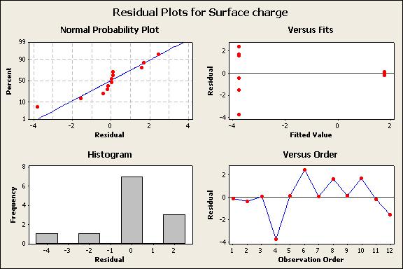
5 4

6 2 Uppgift 2: 7.14 The data shown here represent a single replicate of a 2 5 design that is used in an experiment to study the compressive strength of concrete. The factors are mix (A), time (B), laboratory (C ), temperature (D), and drying time (E). (1) = 700 e = 800 a = 900 ae = 1200 b = 3400 be = 3500 ab = 5500 abe = 6200 c = 600 ce = 600 ac = 1000 ace = 1200 bc = 3000 bce = 3000 abc = 5300 abce = 5500 d = 1000 de = 1900 ad = 1100 ade = 1500 bd = 3000 bde = 4000 abd = 6100 abde = 6500 cd = 800 cde = 1500 acd = 1100 acde = 2000 bcd = 3300 bcde = 3400 abcd = 6000 abcde = 6800 (a) Estimate the factor effects. (b) Which effects appear important? Use a normal probability plot. (c) Determine an appropriate model and analyze the residuals from this experiment. Comment on the adequacy of the model. (d) If it is desirable to maximize the strength, in which direction would you adjust the process variables? 2.1 a By using Minitab we can estimate the factor effects, as seen below. Estimated Effects and Coefficients for Strength Term Effect Coef Constant A B C D E A*B A*C A*D A*E B*C B*D B*E C*D

C*E -62.50-31.25 D*E 225.00 112.50 A*B*C -62.50-31.25 A*B*D 200.00 100.00 A*B*E 50.00 25.00 A*C*D 75.00 37.50 A*C*E 100.00 50.00 A*D*E -87.50-43.75 B*C*D 100.00 50.00 B*C*E -75.00-37.50 B*D*E -62.

7 C*E D*E A*B*C A*B*D A*B*E A*C*D A*C*E A*D*E B*C*D B*C*E B*D*E C*D*E A*B*C*D A*B*C*E A*B*D*E A*C*D*E B*C*D*E A*B*C*D*E b To find out which effects are important a normal plot of the effects is made by using Minitab. From this plot we can conclude that A, B, D, E, AB, DE and ABD appear to be significant. 2.3 c By using the result in b the regression analysis and final model becomes The regression equation is Strength = A B D E AB DE ABD 6

8 Predictor Coef SE Coef T P Constant A B D E AB DE ABD S = R-Sq = 99.1% R-Sq(adj) = 98.9% Analysis of Variance Source DF SS MS F P Regression Residual Error Total Source DF Seq SS A B D E AB DE ABD Obs A Strength Fit SE Fit Residual St Resid

17-1.00 800.0 750.0 110.8 50.0 0.26 18 1.00 1200.0 1212.5 110.8-12.5-0.07 19-1.00 3500.0 3287.5 110.8 212.5 1.11 20 1.00 6200.0 5750.0 110.8 450.0 2.35R 21-1.00 600.0 750.0 110.8-150.0-0.78 22 1.

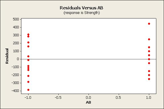
9 R R R denotes an observation with a large standardized residual. Based on the ANOVA, the P-value < α = 0.05 for the regression model, the model appears to be adequate. Looking at the residuals, there are two observation, 20 and 31, that have a residual which is larger than the rest. Though looking at the normal probability plot the residuals appear to be following a straight line. The residuals also look randomly scattered inn the versus fits plot. Looking at the residuals versus the different significant factors we see that they all look good. 8

10 9

11 10

12 11

13 2.4 d The regression equation is Strength = A B D E AB DE ABD. To maximize strength, the variables A, B, D, and E should be increased. Variable C is not significant, thus any level of C would be acceptable. 12

14 3 Uppgift 3: H8.7 An article by J.J. Pignatiello, Jr. and J.S. Ramberg in the Journal of Quality Technology (Vol. 17, 1985, pp ) describes the use of a replicated fractional factorial to investigate the effect of five factors on the free height of leaf springs used in automotive application. The factors are A = furnace temperature, B = heating time, C = transfer time, D = hold down time, and E = quench oil temperature. The data are shown below: A B C D E Free height (a) Write out the alias stucture of this design. What is the resolution of this design? (b) Analyze the data. What factors influence the mean free height? (c) Calculate the range and standard deviation of the free height for each run. Is there any indication that any of these factors affect variability in the free height? (d) Analyze the residuals from this experiment, and comment on your findings. (e) Is this the best possible design for five factors in 16 runs? Specifically, can you find a fractional design for five factors in 16 runs with a higher resolution than this one? 3.1 a Looking at the table above and using Minitab, one can see that the identity operator, I = ABCD. Thus, the resolution is IV. The alias structure of this design is: 13

15 3.2 b Alias Structure I + A*B*C*D A + B*C*D B + A*C*D C + A*B*D D + A*B*C E + A*B*C*D*E A*B + C*D A*C + B*D A*D + B*C A*E + B*C*D*E B*E + A*C*D*E C*E + A*B*D*E D*E + A*B*C*E A*B*E + C*D*E A*C*E + B*D*E A*D*E + B*C*E Doing a design of experiment analysis in Minitab leads to Factorial Fit: Mean free height versus A; B; C; D; E Estimated Effects and Coefficients for Mean free height (coded units) Term Effect Coef Constant A B C D

16 E A*B A*C A*D A*E B*E C*E D*E A*B*E A*C*E A*D*E S = * PRESS = * Analysis of Variance for Mean free height (coded units) Source DF Seq SS Adj SS Adj MS F P Main Effects * * A * * B * * C * * D * * E * * 2-Way Interactions * * A*B * * A*C * * A*D * * A*E * * B*E * * C*E * * D*E * * 3-Way Interactions * * A*B*E * * A*C*E * * A*D*E * * Residual Error 0 * * * Total The normal plot of the effects indicates that the significant factors are A, B, E and the interaction B*E. To study this in more detail all the higher order interactions are excluded except for two-factor interactions. This yields Factorial Fit: Mean free height versus A; B; C; D; E Estimated Effects and Coefficients for Mean free height (coded units) Term Effect Coef SE Coef T P Constant A

17 B C D E A*B A*C A*D A*E B*E C*E D*E S = PRESS = R-Sq = 97.91% R-Sq(pred) = 0.00% R-Sq(adj) = 89.56% Analysis of Variance for Mean free height (coded units) Source DF Seq SS Adj SS Adj MS F P Main Effects A B C D E Way Interactions A*B A*C A*D A*E B*E C*E D*E Residual Error Total Mean free Obs StdOrder height Fit SE Fit Residual St Resid

11 11 7.52000 7.48146 0.06532 0.03854 1.23 12 12 7.64667 7.62562 0.06532 0.02104 0.67 13 13 7.40000 7.37896 0.06532 0.02104 0.67 14 14 7.62333 7.58479 0.06532 0.03854 1.23 15 15 7.20333 7.24396 0.

18 Looking at the P-values, where α = 0.05, for the T-test (or F-test, since the P-values conclude the same for both tests), one can see that the P-values for A, B, E and B*E are below α, thus they are indeed significant and they do influence the mean free height. The free height is thus free height = *A *B *E *B*E, which equals free height = *furnace temperature *heating time *quench oil time *heating time*quench oil time. The versus fits plot for the residuals looks good and the normal probability plot is alright. The value of the residuals are small and nothing is out of the ordinary. 3.3 c The range and standard deviation were calculated by the use of Minitab, the result is in the table below. 17

19 Range Standard deviation Constructing a DOE for the range by using Minitab yields Term Effect Coef Constant A B C D E A*B A*C A*D A*E B*E

20 C*E D*E A*B*E A*C*E A*D*E S = * PRESS = * Analysis of Variance for Range (coded units) Source DF Seq SS Adj SS Adj MS F P Main Effects * * A * * B * * C * * D * * E * * 2-Way Interactions * * A*B * * A*C * * A*D * * A*E * * B*E * * C*E * * D*E * * 3-Way Interactions * * A*B*E * * A*C*E * * A*D*E * * Residual Error 0 * * * Total Looking at the normal plot of the effects it indicates that the interactions C*E and A*D*E are significant. Since A*D*E is aliased with B*C*E, B*C*E was included in the analysis, this leads to Factorial Fit: Range versus A; B; C; E Estimated Effects and Coefficients for Range (coded units) Term Effect Coef SE Coef T P Constant A B C E B*C B*E C*E

21 B*C*E S = PRESS = R-Sq = 86.68% R-Sq(pred) = 30.43% R-Sq(adj) = 71.46% Analysis of Variance for Range (coded units) Source DF Seq SS Adj SS Adj MS F P Main Effects A B C E Way Interactions B*C B*E C*E Way Interactions B*C*E Residual Error Total Obs StdOrder Range Fit SE Fit Residual St Resid

Looking at the P-values in the ANOVA table for the main effects and interactions one can see that the two- and three-way interactions are significant, thus all of the main effects will be significant

06812*C*E + 0.06937*B*C*E, which equals range = 0.21937 + 0.05688*furnace temperature - 0.06312*heating time + 0.01313*transfer time - 0.00687*quench oil temperature + 0.

22 Looking at the P-values in the ANOVA table for the main effects and interactions one can see that the two- and three-way interactions are significant, thus all of the main effects will be significant as well, even though the P- values for C and E are not in agreement. The range thus becomes range = *A *B *C *E *B*C *B*E *C*E *B*C*E, which equals range = *furnace temperature *heating time *transfer time *quench oil temperature *heating time*transfer time *heating time*quench oil temperature *transfer time*quench oil temperature *heating time*transfer time*quench oil temperature. The residuals in the table are small and both the normal probability plot and the versus fits for the residuals look good. Constructing a DOE for the standard deviation by using Minitab yields Factorial Fit: Standard deviation versus A; B; C; D; E 21

23 Estimated Effects and Coefficients for Standard deviation (coded units) Term Effect Coef Constant A B C D E A*B A*C A*D A*E B*E C*E D*E A*B*E A*C*E A*D*E S = * PRESS = * Analysis of Variance for Standard deviation (coded units) Source DF Seq SS Adj SS Adj MS F P Main Effects * * A * * B * * C * * D * * E * * 2-Way Interactions * * A*B * * A*C * * A*D * * A*E * * B*E * * C*E * * D*E * * 3-Way Interactions * * A*B*E * * A*C*E * * A*D*E * * Residual Error 0 * * * Total

24 Standard SE St Obs StdOrder deviation Fit Fit Residual Resid * * * * * * * * * * * * * * * * * * * * * * * * * * * * * * * * Looking at the normal plot of the effects it indicates that the factors A, B and the interactions C*E and A*D*E are significant. Since A*D*E is aliased with B*C*E, B*C*E was included in the analysis, this leads to Factorial Fit: Standard deviation versus A; B; C; E Estimated Effects and Coefficients for Standard deviation (coded units) Term Effect Coef SE Coef T P Constant A B C E B*C B*E C*E B*C*E S = PRESS = R-Sq = 88.63% R-Sq(pred) = 40.62% R-Sq(adj) = 75.65% Analysis of Variance for Standard deviation (coded units) Source DF Seq SS Adj SS Adj MS F P Main Effects A B C E

25 2-Way Interactions B*C B*E C*E Way Interactions B*C*E Residual Error Total Standard Obs StdOrder deviation Fit SE Fit Residual St Resid Looking at the P-values in the ANOVA table for the main effects and interactions one can see that the two- and three-way interactions are significant, thus all of the main effects will be significant as well, even though the P- 24

26 values for C and E are not in agreement. The standard deviation thus becomes standard deviation = *A *B *C *E *B*C *B*E *C*E *B*C*E, which equals standard deviation = *furnace temperature *heating time *transfer time *quench oil temperature *heating time*transfer time *heating time*quench oil temperature *transfer time*quench oil temperature *heating time*transfer time*quench oil temperature. The residuals in the table are small and the versus fits for the residuals look good. The normal probability plot does not appear to be satisfactory. 3.4 d Some of the residuals have already been discussed above, the rest, for the free height, follow here 25

27 26

28 27

The normal probability plot and the versus fits plot for the free height both look good. All the residuals in the plots for the different factors look good too. 3.

29 The normal probability plot and the versus fits plot for the free height both look good. All the residuals in the plots for the different factors look good too. 3.5 e This is not the best possible design for five factors in 16 runs. It is possible to construct a resolution V design by setting the generator equal to the highest order interaction, ABCDE, thus the design would have a higher resolution. 28

30 4 Uppgift 4: 7.40 In their book, Empirical Model Building and Response Surfaces (Hoboken, NJ: John Wiley Sons, 1987), G. E. P. Box and N. R. Draper describe an experiment with three factors. The data shown in the following table are a variation of the original experiment on page 247 of their book. Suppose that these data were collected in a semiconductor manufacturing process. x 1 x 2 x 3 y 1 y (a) The response y 1 is the average of three readings on resistivity for a single wafer. Fit a quadratic model to this response. (b) The response y 2 is the standard deviation of the three resistivity measurements. Fit a linear model to this response. (c) Where would you recommend we set x 1, x 2, and x 3 if the objective is to hold mean resistivity at 500 and minimize standard deviation? 4.1 a By using Minitab a quadratic model was fitted to y 1, as seen below. Estimated Regression Coefficients for y1 Term Coef SE Coef T P 29

31 Constant x x x x1*x x2*x x3*x x1*x x1*x x2*x S = PRESS = R-Sq = 92.69% R-Sq(pred) = 74.92% R-Sq(adj) = 88.81% Analysis of Variance for y1 Source DF Seq SS Adj SS Adj MS F P Regression Linear x x x Square x1*x x2*x x3*x Interaction x1*x x1*x x2*x Residual Error Total Obs StdOrder y1 Fit SE Fit Residual St Resid R

32 R R denotes an observation with a large standardized residual. Estimated Regression Coefficients for y1 using data in uncoded units Term Coef Constant x x x x1*x x2*x x3*x x1*x x1*x x2*x In both the estimated regression and ANOVA we find that the P-value < α = 0.05 for the linear terms and interaction terms, they appear to be significant. The P-value < α = 0.05 for x 1, x 2, x 3, x 1 x 2 and x 1 x 3, thus they are significant for the model. The P-value for x 2 x 3 is 0.064, which is really close to α, but I m still putting it as insignificant. The quadratic model for y 1 is y 1 = x x x x 1 x x 1 x 3. Looking at the normal probability plot and the versus fits plot of the residuals, they both look good, the residuals are all scattered in the versus fits plot and they re following a somewhat straight line in the normal proability plot. Observations 9 and 19 have larger residuals than the rest. 31

33 4.2 b By using Minitab a linear model was fitted to y 2, as seen below. Estimated Regression Coefficients for y2 Term Coef SE Coef T P Constant x x x S = PRESS = R-Sq = 36.71% R-Sq(pred) = 11.32% R-Sq(adj) = 28.45% Analysis of Variance for y2 Source DF Seq SS Adj SS Adj MS F P Regression Linear x x x Residual Error Total Obs StdOrder y2 Fit SE Fit Residual St Resid

34 R R denotes an observation with a large standardized residual. Estimated Regression Coefficients for y2 using data in uncoded units Term Coef Constant x x x In both the estimated regression and ANOVA we find that the P-value < α = 0.05 for the linear terms, they appear to be significant. The P-value < α = 0.05 for x 3, thus it is significant for the model. The linear model for y 2 is y 2 = x 3. Looking at the versus fits plot of the residuals, it looka good, the residuals are all scattered in the versus fits plot. Observations 19 has a larger residual than the rest. The residuals in the normal probability plot seem to follow a slight curvature instead of a straight line. 33

4.3 c The formula for the standard deviation is y 2 = 47.9952 + 29.1917 x 3, where 1 < x 3 < 1. To minimize the standard deviation we pick x 3 = 1.

Since x 3 = 1 I choose x 2 = 0, so x 2 and x 3 are in the smallest area, with a minimized standard deviation.

35 4.3 c The formula for the standard deviation is y 2 = x 3, where 1 < x 3 < 1. To minimize the standard deviation we pick x 3 = 1. A contour plot was made of y 2 vs x 2 and x 3. From this contour plot we see that y 2 has the smallest area to the bottom left. Since x 3 = 1 I choose x 2 = 0, so x 2 and x 3 are in the smallest area, with a minimized standard deviation. To attain the desired level of 500 for the mean, the quadratic equation found in part a will be solved with y = 500, x 2 = 0 and x 3 = 1 to find x 1. We have 500 = x x 1 which leads to an x 1 3 in this particular situation (x 2 = 0, x 3 = 1, y = 500). 34

36 5 Uppgift 5: H12.1 An article in Industrial Quality Control (1956, pp. 5-8) describes an experiment to investigate the effect of glass type and phosphor type on the brightness of a television tube. The response measured is the current necessary (in microamps) to obtain a specified brightness level. The data are shown here. Analyze the data and draw conclusions. 5.1 Analysis Phosphor Type Glass Type To check if the factors (glass type, phosphor type) influence the brightness level a Two-way ANOVA is made, where we look at the equality of row treatment effects (glass type) { H 0 : τ 1 = τ 2 = 0 H 1 : τ i 0 for at least one i and the equality of column treatment effects (phosphor type) { H 0 : β 1 = β 2 = β 3 = 0 H 1 : β i 0 for at least one i. We also want to know if the row and column treatments interact { H 0 : (τβ) ij = 0 H 1 : (τβ) ij 0 for at least one ij. The null hypothesis, H 0, is rejected if the P-value < α, here α = Inserting the data in Minitab and doing a Two-way ANOVA yields: 35

37 Two-way ANOVA: Brightness level versus Glass Type; Phosphor Type Source DF SS MS F P Glass Type Phosphor Type Interaction Error Total S = R-Sq = 96.08% R-Sq(adj) = 94.44% Individual 95% CIs For Mean Based on Glass Pooled StDev Type Mean (--*-) (--*-) Individual 95% CIs For Mean Based on Phosphor Pooled StDev Type Mean ( * ) ( * ) ( * ) Phosphor Type Glass Type Brightness level RESI

38 Residual Frequency Residual Percent Residual Residual Plots for Brightness level 99 Normal Probability Plot Versus Fits Residual Fitted Value Histogram Versus Order Residual Observation Order Residuals Versus Glass Type (response is Brightness level) Glass Type

39 Residual Residuals Versus Phosphor Type (response is Brightness level) Phosphor Type

40 We find that the P-value for glass type is 0, which is less than α = 0.05, the null hypothesis can be rejected, thus glass type is significant and affects the brightness level. The P-value for phosphor type is 0.004, which is less than α = 0.05, the null hypothesis can be rejected, thus phosphor type is significant and affects the brightness level. The P-value for the interaction between the glass- and phosphor type is 0.318, which is bigger than α = 0.05, thus the null hypothesis cannot be rejected and the interaction is insignificant and there is no effect from the interaction on the brightness level. The normal probability plot for the brightness level looks alright, except for one of the residuals of phosphor- and glass type 2, where the residual has the value of 15, which can be seen in the column RESI1. It stands out a bit compared to the others, but most of the residuals follow a straight line, which indicates that the model seems to fit the data well. The coefficient of determination, R 2 = , which is very high, meaning that the model is well fitted to the data material. The versus fits plot doesn t show any particular pattern for the residuals. There might be a slight tendency for the variance of the residuals to increase. Looking at the plots of the residuals versus glass- and phosphor type respectively, one can see that the two plots both have a slight inequality of variance. And the combination of glass type 2 and phosphor type 2 might have a larger variance than the other combinations. 39

a) Prepare a normal probability plot of the effects. Which effects seem active?

a) Prepare a normal probability plot of the effects. Which effects seem active? Problema 8.6: R.D. Snee ( Experimenting with a large number of variables, in experiments in Industry: Design, Analysis and Interpretation of Results, by R. D. Snee, L.B. Hare, and J. B. Trout, Editors,