Analytical and Numerical Modeling of Delamination Evolution in Fiber Reinforced Laminated Composites Subject to Flexural Loading

Transcription

1 Analytical and Numerical Modeling of Delamination Evolution in Fiber Reinforced Laminated Composites Subject to Flexural Loading by Jiawen Xie A dissertation submitted in partial fulfillment of the requirements for the degree of Doctor of Philosophy (Aerospace Engineering and Scientific Computing) in the University of Michigan 217 Doctoral Committee: Professor Anthony M. Waas, Co-Chair Associate Professor Veera Sundararaghavan, Co-Chair Professor Krishna Garikipati Associate Professor Nakhiah Goulbourne Mostafa Rassaian, Boeing Research & Technology

2 Jiawen Xie 217

3 To my family ii

4 ACKNOWLEDGMENTS My deepest gratitude is to my advisor, Professor Anthony Waas, who has guided me into this field. He encouraged me to advance my career into a higher level after I earned my Master s degree, and finally to become the author of this dissertation. I remember those days when he enlightened me on possible pathways in my quest to seek answers, and those nights when I trod through them with the same persistence passed on. I will be always inspired by his creativeness, incisiveness and enthusiasm. My thanks also go to Professor Veera Sundararaghavan as the co-chair, and Professor Krishna Garikipati and Professor Nakhiah Goulbourne as dissertation committee members, for their insightful comments and suggestions during my drafting of this dissertation. Dr. Mostafa Rassaian also provided me with numerous industry-based ideas and advice in my research, and I owe him my great gratitude. It was a great pleasure to work with my colleagues in the Composite Structures Laboratory. Experimental work done by Solver Thorsson, Ashith Joseph, Jaspar Marek are greatly helpful for developing and validating the analysis in this dissertation. Special thanks go to my officemates, Dr. Dianyun Zhang, Dr. Marianna Maiaru, and Dr. Paul Davidson. I will always reflect all the valuable discussions and joyful moments filled with scent of coffee. I have received generous help from Dr. Wu Xu on numerical simulations and brilliant suggestions on extending my analysis. I will never forget the days spent with Dr. Wooseok Ji, Dr. Pavana Prabhakar, Dr. Royan D Mello, Dr. Nhung Nguyen, Dr. Pascal Meyer, Dr. Akinori Yoshimura, Cyrus Kosztowny, Armanj Hasanyan, Deepak Patel, David Singer, Alastair Croxford, Kelsey Herrmann, Shiyao Lin, and Kuo Tian. I sincerely thank the staff of the Department of Aerospace Engineering at the University of Michigan and the Department of Aeronautics&Astronautics at the University of Washington for their tremendous support for the students. Special thanks go to Ms. Denise Phelps and Ms. Bonnie Bryant who provided me with countless help on academic program coordination. The research of this dissertation was supported in part through computational resources and services provided by Advanced Research Computing at the University of Michigan and the Hyak supercomputer system at the iii

5 University of Washington. Last but not least, I would like to thank my beloved grandparents, parents and husband, Haolu. This journey would not have been possible without your love, encouragement, and support. I am grateful for the financial support from The Boeing Company. Thanks to Dr. Mostafa Rassaian, Dr. Salvatore Liguore, Dr. Joseph Schaefer, and Dr. Brian Justusson for the helpful discussions in regular past meetings. iv

6 TABLE OF CONTENTS Dedication Acknowledgments ii iii List of Figures viii List of Tables List of Appendices Abstract xii xiii xiv Chapter 1 Introduction Motivation Research Objective and Thesis Outline D Elastodynamic Solutions for Impacted Laminated Composites Panels Introduction General Elasticity Solutions Governing Equations Frequencies and Mode Shapes Vibrational Response Impact Responses Other Theories and Modeling Equivalent Single-layer Theories Finite Element Modeling Results and Discussions Natural Frequencies and Mode Shapes Impact Responses Conclusions Predictions of Delamination Growth for Quasi-static Loading of Composite Laminates Introduction D Elasticity Approach v

7 3.2.1 Governing Equations Contact Models at Delaminated Interface Solution Technique Modeling Three-point Bend Tests Predictions of Delamination Growth Modified Classical Lamination Theory Governing Equations Contact Models and Solutions Other Theories and Modeling Simple Fracture Model Finite Element Modeling Results and Discussions Transverse Stress Analysis Delamination Threshold Loads Load-displacement Responses Conclusions Closed-form Solutions for Cohesive Zone Modeling of Delamination Toughness Tests Introduction General Cohesive Zone Modeling Solutions of DCB Test (Mode I Fracture) Solution Forms Solution Technique for Bi-linear Cohesive Law Solution Technique for Multi-linear Cohesive Law Solutions of ENF Test (Mode II Fracture) Solution Forms Solution Technique Solutions of MMB Test (Mixed-mode I/II Fracture) Method without Superposition Method of Superposition Results and Discussions Applications of a Bi-linear Traction-separation Law The MMB Configuration Influence of the Shape of the Cohesive Law Conclusions Estimating the Process Zone Length of Fracture Tests Used in Characterizing Composites Introduction General Problem Solutions of the DCB Configuration by Williams and Hadavinia Solutions of the ENF Configuration Solutions of the MMB Configuration Results and Discussions vi

8 5.6.1 The DCB and ENF Configuration The MMB Configuration Conclusions Analytical Predictions of Delamination Threshold Load of Laminated Composite Plates Subject to Flexural Loading Introduction Elastic Bending of a Laminated Plate Combined with Cohesive Zone Modeling Formulations Initiation of Delaminations on Pristine Interfaces Propagation of Existing Delaminations Results and Discussions Conclusions Concluding Remarks Conclusions Suggestions for Future Studies Appendices Bibliography vii

9 LIST OF FIGURES 1.1 Damage types in impacted fibre reinforced laminates A general cohesive constitutive law of mode I fracture Geometry of a laminated composite panel Parabolic impact loading FE model used for numerical simulations of impact events Fourier expansions of impact loading in space for aspect ratio of 6 and Half-time snapshots of impact response of stress σ z at the central line x = L/ Half-time snapshots of impact response of stress σ z off the central area Half-time snapshots of impact response of stress τ xz at the left end x = Half-time snapshots of impact response of stress τ xz off the central area Transverse stress history of 3-layer laminate (/9/) D illustration of the pre-delaminated composite panel The piecewise linear spring model Configuration of three-point bend tests on a pre-delaminated panel Four-section partition of a pre-delaminated composite panel in modified CLT Free body diagrams of modified CLT Simple fracture models Transverse stress distributions at delaminated interface of specimens with mid-plane delamination length.3l Transverse shear stress distributions near the crack tip at delaminated interface of specimens with mid-plane delamination length of.3l The convergence study on average transverse stresses of 32-ply specimen with mid-plane delamination length Variations of delamination threshold load with existing centre delamination length of 12-ply orthotropic laminated panel Variations of delamination threshold load with existing centre delamination length of 32-ply cross-ply laminated panel Errors between simple fracture models and 2D elasticity theory using general contact model and fracture mechanics based failure criterion Load-displacement responses for 12-ply specimen with delamination length of.5l Variations of load-displacement responses with delamination length for 12-ply and 32-ply specimen with mid-plane delamination viii

10 4.1 Geometry of a pre-cracked laminated composite panel Free-body diagrams of two sub-laminates connected by the cohesive zone A piecewise linear cohesive constitutive law of mode I fracture Diagram and variables of the DCB test Three stages of the flexural response when applying a bi-linear cohesive law The algorithm to find equilibrium (EQM) state in the DCB configuration by using the triangular (bi-linear) cohesive law The algorithm to find equilibrium state in the DCB configuration by using the multi-linear cohesive law Diagram and variables of the ENF test Linearized traction-separation law of mode II fracture Diagram and variables of the MMB test Possible combinations of different sections in the MMB configuration by using bi-linear traction-separation laws for both mode I and II Algorithm to find equilibrium state in the MMB configuration by using triangular (bi-linear) cohesive laws for both mode I and II The superposition method of the MMB configuration General algorithm to find equilibrium state in the MMB configuration by the superposition method with arbitrary multi-linear cohesive laws of mode I and mode II Load-displacement response with crack length markers as well as the maximum load of linear response P and the failure load P c Parametric study of strength on the load-displacement response Parametric study of strength and crack length on the failure load Parametric study of fracture energy on the load-displacement response Process zone length as the crack advances Parametric study of strength and fracture energy on the process zone length Load-displacement responses of the MMB test with three different loading positions Mode mixity of the MMB configuration with three different loading positions Process zone length of mode I and II failure during the MMB test with three different loading positions Load-displacement responses and mode mixity of the MMB configuration by using the method of superposition Mode mixity and process zone length corresponding to the initial crack length of the MMB configuration by using the method of superposition with three failure criteria Variations of the shapes of bi-linear cohesive laws Load-displacement responses of the DCB and ENF configuration by varying the shape of bi-linear traction-separation law Process zone length of the DCB and ENF configuration by varying the shape of bi-linear traction-separation law ix

11 4.29 Multi-linear cohesive laws for mode I used in the numerical evaluations Load-displacement responses of the DCB configuration by using different cohesive laws Load-displacement responses of the ENF configuration by using different cohesive laws Process zone length by using different cohesive laws Configuration and partition of a pre-crack laminated composite panel Traction-separation laws used for modeling pure mode fracture Diagram and variables of the DCB test Diagram of the reduced DCB problem by the assumption of mid-plane symmetry Diagram and variables of the ENF configuration Superposition method of the MMB configuration Load-displacement responses of pure-mode fracture toughness tests Parametric study on the process zone length of the DCB configuration Parametric study on the process zone length of the ENF configuration Load-displacement responses of the MMB test with three different loading positions Mixed-mode cohesive laws corresponding to the crack length a = 3 mm Cohesive traction distribution in the fully developed cohesive zone with the crack length a = 3 mm Variations of mode mixity and mixed-mode strength values with lever length Relations between the process zone length and the mode mixity A simply supported laminated plate under transverse loading condition Modeling of a laminated plate with a potential crack interface A linear elastic-brittle traction-separation law of mode II/III fracture Configuration of quasi-static face-on impact tests FE model of the quasi-static face-on impact test of a laminated composite plate Convergence studies of the stiffness on number of series considered in the Rayleigh-Ritz method FE model with a cohesive layer Convergence studies of the stiffness and the delamination threshold load on number of series considered in the Rayleigh-Ritz method Normalized interfacial shear traction distribution over the interface of laminate with stacking sequence () 2 by the Rayleigh-Ritz method (left) and FE simulations (right) Normalized interfacial shear traction distribution over all interfaces of laminate with stacking sequence (/9/+45/-45//-45/+45/9/) by the Rayleigh-Ritz method (left) and FE simulations (right) x

12 A.1 The crack band model with non-linear strain measures and linear tractionseparation law A.2 Intra-lamina failure modes of fiber-reinforced laminated composites that are modeled as homogenous anisotropic material with the crack band model A.3 Failure progression observed in experiments of the type-a laminate specimens (-45 8 /+45 8 /9 8 / 8 ) s A.4 Failure progression observed in experiments of the type-b laminate specimens (+45 8 /-45 8 / 8 /9 8 ) s A.5 FE simulations of failure progression the type-a laminate specimens ( /+45 8 /9 8 / 8 ) s A.6 FE simulations of failure progression the type-b laminate specimens (+45 8 /-45 8 / 8 /9 8 ) s B.1 Load-displacement responses of laminates (+45 4 /-45 4 / 4 /9 4 ) s with two different width, 12.7 mm and 5.8 mm, by using different theories and elements B.2 Parametric studies of the fiber orientation θ on the flexural stiffness of laminates (+θ 4 /-θ 4 / 4 /9 4 ) s by using different theories and numerical models xi

13 LIST OF TABLES 2.1 Homogenized lamina properties used Fundamental natural frequencies aspect ratio of Fundamental natural frequencies for aspect ratio of Converging tolerance [%] of transient solution by exponential and cubic steady-state solution function Homogenized lamina properties and interface fracture properties of the material used published three-point bend test Homogenized lamina properties and interface fracture properties Normalized stiffness parameters for the contact springs Homogenized lamina properties and interface fracture properties of IM7/8552 graphite/epoxy Key dimensions used in numerical evaluations Process zone length calculated by various methods Results of the MMB configuration with three different loading positions and crack length a = 3 mm Stiffness predicted by the Rayleigh-Ritz method (8 8 series) and FE simulations Stiffness and critical loads predicted by the Rayleigh-Ritz method (8 8 series) and FE simulations of laminate with stacking sequence () Stiffness and critical loads predicted by the Rayleigh-Ritz method (8 8 series) and FE simulations of laminate with stacking sequence (/9/+45/- 45//-45/+45/9/) A.1 Stacking sequences and dimensions of laminate specimens A.2 Homogenized lamina properties and fracture properties of IM7/8552 graphite/epoxy B.1 Dimensions of laminate xii

14 LIST OF APPENDICES A Numerical Simulations of Three-point Bend Tests of Laminated Beams B 3D Effects of Laminated Beam Containing Off-axis Angle Plies. 19 C Simple Beam Theory (SBT) Solutions D Derivation of Additional Continuity in Estimated CZM Solutions 199 E Coefficients of Estimated Solutions of CZM F Transverse Shear Stiffness for Laminated Plates G Closed-form Solutions for Cross-ply Laminates H The Rayleigh-Ritz Method with the Classical Lamination Theory (CLT) xiii

15 ABSTRACT Analytical and Numerical Modeling of Delamination Evolution in Fiber Reinforced Laminated Composites Subject to Flexural Loading by Jiawen Xie Co-Chairs: Anthony M. Waas and Veera Sundararaghavan Delamination or interfacial debonding is a common failure mode in composite (fiber reinforced and layered) structures and other general multi-layered structures subject to a variety of loading conditions, such as bending or low-velocity impact by foreign objects. A better understanding of delamination evolution and its relation to geometry of the structure, lamina stacking sequences, size of existing crack, and interfacial properties is very helpful in design and repair processes. In recent years, finite element (FE) simulations that use cohesive elements have found wide appeal in modeling onset and growth of the delamination. Despite its popularity, some common numerical issues in cohesive zone modeling (CZM) have not been fully addressed, such as instability, convergence difficulties, and length-scale issues due to discretization. Therefore, analytical solutions of CZM are important to obtain a comprehensive understanding of modeling artifacts and a platform for acquiring computationally efficient results, as well as to provide benchmark cases and suggest element sizes and mesh densities when FE simulations are to be used. The focus of this research is to analyze flexural responses and delamination evolution in laminated composites under transverse loading conditions. Analytical solutions were formulated and computed for various flexural test configurations of laminated beam and plate structures. The results, including load-displacement responses and delamination threshold loads, were cross-checked with experiments and FE simulations. xiv

16 Two-dimensional (2D) elasticity theory for laminated panels was extended to analyze elastodynamic responses of pristine panels and quasi-static responses of predelaminated panels. Stress distributions, load-displacement responses, and delamination threshold loads calculated per the 2D elasticity theory for cross-ply laminates were found in good agreement with FE simulations with plane-strain elements and existing experimental data. Further investigations showed that the 2D elasticity theory is not amenable to a closed-form solution for laminates containing off-axis angle plies due to three-dimensional (3D) states of stress. Closed-form solutions for CZM within a framework of classical lamination theory (CLT) were developed, for three popular delamination toughness characterization tests, including mode I double cantilever beam (DCB) test, mode II end notched flexure (ENF) test, and mixed-mode I/II bending (MMB) test of laminated beams. Following the concept of CZM, a laminated panel was considered as an assembly of two sub-laminates connected by a virtual deformable layer with infinitesimal thickness. Comprehensive parametric studies were performed on crack growth responses and process zone lengths, revealing their relations to delamination lengths, cohesive parameters, shapes of the traction-separation laws, and mode mixity, controlled by external loading conditions. The studies with laminated beams were simplified by considering linear damage (quasi-brittle) traction-separation laws that consist of only one quasi-brittle softening segment, so that closed-form expressions can be obtained, serving as a quick estimation of the flexural responses and the process zone lengths for the three delamination toughness characterization tests. Known for its dependence on the mode mixity, material properties, and interfacial fracture properties, the process zone lengths were found as a system parameter that is also influenced by specimen geometry, such as thickness and crack lengths. Based on parametric studies and comparisons against FE simulations, suggestions for estimating the process zone lengths were provided. Analytical solutions for CZM were further extended to analyze laminated plates subject to flexural loading. Due to extension-shear couplings, the Rayleigh-Ritz method was used to determine approximate solutions for an elastic response and delamination evolution of laminates with arbitrary stacking sequences, within a framework of either CLT or first-order shear deformation theory (FSDT). Configurations of quasi-static face-on impact tests were analyzed as an example. The results, including elastic stiffness of flexural responses, traction distributions over potential crack interfaces, threshold loads of the delamination, and initiating locations of the delamination, were found in good agreement with FE simulations. xv

17 The analytical solutions formulated herein can be used with confidence to study general multilayered structures, and be extended to consider other loading conditions as well as other boundary conditions. xvi

18 CHAPTER 1 Introduction 1.1 Motivation During manufacturing processes and services, unexpected impacts on fiber reinforced laminated composite structures by foreign objects, such as dropped tools, runway debris, and service vehicles, can occur. Damage induced by those impact events is a major concern in designing laminated composite structures because it can be barely visible while largely altering the functionality of a designed structure in terms of stiffness and strength [1]. Common failure modes of impact damage are matrix cracking, delamination and fiber breakage, [2], as shown in Figure 1.1. Delamination is particular serious because it has a major influence on flexural stiffness and buckling failure. To maximize the design capacity, it is important to have reliable tools to predict delamination evolution in laminated composites subject to flexural loading and low-velocity impacts. The predictive tools for delaminated structural response are also one step towards virtual engineering in design, manufacturing and testing that is fully based upon computer aided modeling and simulations. Though real physical experiments are valuable and necessary for characterizing and validating purposes, virtual engineering provides an efficient way to explore more design possibilities with lower costs of prototyping, testing and optimization. From a viewpoint of fracture analysis, delamination is driven by interlaminar normal (peel) stress, characterized as mode I, and interlaminar shear stresses, denoted as mode II and III for in-plane and out-of-plane cases, respectively [3]. To predict initiation and propagation of delaminations, a stress- or strain-based continuum damage mechanics approach is intuitive. The approach can provide time and locations of delamination evolution by comparing the interlaminar stresses or strains to relevant strength parameters that are measured from experiments. In this sense, predictions of the stress- or strain-based approach heavily rely on the accuracy of stresses cal- 1

19 Figure 1.1: Damage types in impacted fibre reinforced laminates [2]. culated, especially transverse stresses. Analytical approaches using elasticity theory [4, 5, 6] can accurately predict transverse stress distributions of multilayered composites subject to flexural loading. The elasticity approaches directly solve layer-wise displacement fields from force and moment equilibrium, strain-displacement relations, and constitutive laws in continuum mechanics with appropriate boundary conditions and continuity conditions between layers. However, analytical solutions using the elasticity approaches are only available for a limited class of problems. Simplified analytical theories for multilayered composites reduce the elasticity approaches to beam and plate theories based formulations by making appropriate assumptions on the width and the thickness directions of composite structures. They provide good approximations for the displacement fields and stiffness of structures. Representive simplified theories are classical lamination theory (CLT) and first-order shear deformation theory (FSDT), distinguished by whether transverse shear deformation is prohibited or allowed [7]. Unfortunately, most simplified theories cannot provide satisfactory stress distributions in the through-the-thickness direction, making them useless in the continuum damage mechanics approach for predicting delaminations. Additionally, by analyzing a problem of an infinite sheet with semi-infinite cracks subjected to far-field loading conditions, solutions based on linear elastic fracture mechanics (LEFM) have shown that the stress field near the crack tip has a characteristic r 1/2 singularity where r is the distance from the crack tip [3]. In spite of its simplicitiy, the LEFM-based solutions suggest a stress concentration with very high gradients near the crack tip, where stresses can be difficult to be accurately captured by both analytical solutions and finite element (FE) based simulations. 2

20 σ σ c G Ic w w c w Figure 1.2: A general cohesive constitutive law of mode I fracture. The law for mode II is similar (σ τ, w u) but antisymmetric with respect to the origin. Instead of directly calculating stresses, LEFM-based solutions [8, 9] and FE methods such as virtual crack closure technique (VCCT) [1, 11] consider that the crack can have self-similar growth when the change of potential energy per increment of crack advance, referred to as energy release rate, satisfies energy-based criteria. The energy methods work well in studying propagation of an existing delamination while they have limited capability in predicting delamination initiation if the crack initiating location is unknown. In recent years, FE methods with cohesive elements have been advanced to predict both initiation and propagation of cracks at potential crack interfaces by applying traction-separation laws that combine strength and energy based criteria, without previous knowledge of the crack location and growth path. The original cohesive fracture concept was proposed by Barenblatt [12, 13] who considered additional molecular cohesive forces holding the upper and the lower surfaces of a narrow zone ahead of the crack tip. As a result, the stress singularity near the crack tip is removed. If the cohesive forces distributed in the narrow zone equals a constant value of yield stress, the concept can be considered identical to Dugdale s strip yield model [14]. The Dugdale-Barenblatt model was first adopted and implemented in the finite element framework to study crack growth in concrete in Ref. [15], where finite geometry was fully considered and the cohesive constitutive law independent of the continuum material properties was defined more generally as a nonlinear traction-separation relation. As shown in Figure 1.2, the relation indicates that as the separation increases, the traction across the potential crack interface reaches a maximum, then decreases, and eventually vanishes signifying the onset of crack propagation. The modeling technique of cohesive elements has received continuous improvements dur- 3

21 ing the last four decades in different aspects, such as characterizations of cohesive constitutive laws [16, 17, 18, 19, 2, 21], the implementation of mixed-mode failure modeling [18, 21, 22, 23, 24, 25, 26] and the development of discrete cohesive elements [18, 27, 28]. Since the cohesive zone modeling (CZM) is a generalized method that allows using different shapes of cohesive laws to simulate various interfacial behavior, it has been widely accepted as a tool to predict the onset and growth of delamination or interfacial debonding for fiber reinforced laminated composites [29, 3, 31, 32, 33, 34] and sandwich structures [35], as well as other applications of general multi-layer composites, such as hot mix asphalt pavement [36] and multi-layer coatings [37]. The method has also been extended to model non-interfacial crack propagation along preassigned potential crack paths [38] and used in analyzing impact damage [39]. Despite its popularity, some numerical issues of CZM have not been fully solved. First, numerical instability and convergence difficulties at the onset of crack propagation are still common, especially when extreme values of the parameters such as initial elastic stiffness, strength and fracture energy are assigned to simulations, preventing a comprehensive understanding of modeling artifacts. Second, the relationship between process zone lengths and cohesive parameters remains to be studied, so that a universal solution to determine the process zone length can be obtained. The process zone length, defined by the length over which the cohesive zone enters the post-peak degradation process, is a key meshing parameter for finite element simulations that use cohesive elements. Past literature has demonstrated that it is necessary to use three or more cohesive elements to correctly capture crack propagation and maintain mesh objectivity [4, 41]. Therefore, analytical solutions of CZM are gaining attention since they provide insight into the mechanics of delamination growth, and a platform for accessing computationally efficient results free from length-scale issues due to discretization. Following Kanninen s original idea [42], analytical solutions derived from beam theories introduce springs in normal and tangential directions connecting the upper and lower surfaces of potential crack interfaces where the cohesive zone is placed in numerical simulation. Since delamination evolution at the potential crack interfaces is essentially governed by separation displacements between those two surfaces, the drawback in predicting stress distributions of beam or plate theories is avoided. The solutions are available for many delamination characterizing tests, such as mode I double cantilever beam (DCB) tests [43, 44, 45, 46, 47], mode II end notched flexure (ENF) tests [48, 46], mixed-mode I/II bending (MMB) tests [46, 49], asymmetric DCB (ADCB) tests [5] and moment loaded DCB (MLDCB) tests [51, 47, 52, 53]. However, 4

22 most of the solutions only discuss a simple application of linear elastic-brittle springs, namely no softening behavior, and focus on pre-failure responses. More general analytical CZM solutions are difficult to develop because of the nonlinearity introduced by traction-separation laws. It is also worth pointing out that, helpful as analytical CZM solutions and FE simulations using cohesive elements in modeling delamination evolution, it is still and will be under debate for a long time whether CZM correctly reflects the actual physics of crack propagation. Attempts have been made to develop new cohesive laws based on failure mechanisms at the atomic level [19, 21, 54] and to numerically study influences of different existing laws [55, 56]. Therefore, it is necessary to develop an evaluation tool based on general analytical CZM solutions that can provide accurate results with arbitrary application of nonlinear cohesive laws. In addition, analytical CZM solutions found in past literature are restricted to beam configuration under some simplifications on stacking sequences and delamination locations. To analyze delamination evolution in general laminated plates, which is a more practical concern in design processes, it is also necessary to extend the solutions to higher dimensions with less restrictions. Besides crack growth responses, process zone length is another important outcome of analytical CZM solutions. Analytical studies of process zone lengths found in the literature fall into two categories: strip yield model and large-scale crack bridging model [57, 29, 4, 41]. The strip yield model analyzes infinite geometries while the large-scale crack bridging model is limited to cohesive laws with infinite initial stiffness. Therefore, it is of interest to develop analytical solutions that consider the same setting adopted in FE simulations of finite geometry and use nonlinear cohesive laws consisting of elastic and softening segments to provide benchmark solutions of flexural responses and process zone lengths under mode I, mode II and mixed-mode loading conditions. 1.2 Research Objective and Thesis Outline In this dissertation, various analytical solutions of flexural responses and delamination evolution of fiber reinforced laminated composites subject to flexural loading are presented. Numerical FE simulations are subsequently used for cross-checking and validating analytical solutions and computations. The dissertation can be broadly divided into two parts. The first part focuses on analytical approaches using elasticity theory. Chapter 2 extends two-dimensional (2D) elasticity theory to analyze elastodynamic responses 5

23 of laminated wide panels subject to dynamic loading. Natural frequencies and mode shapes of free vibration are first extracted. Inspired by a transformation technique for solving a special class of partial differential equations, forced vibration problems of impacted laminated panels are solved using an eigenfunction expansion technique. Chapter 3 presents an exact, quasi-static analysis of pre-delaminated composite panels under transverse loading conditions. A piecewise linear spring model and a shear bridging model are, respectively, used to simulate normal contact and shear frictional behavior between the interfaces of the existing delamination. Both analysis provide closed-form solutions of displacement fields and stress distributions. To predict delamination propagation, strength- and energy-based criteria are considered in Chapter 3. Calculated load-displacement responses and delamination threshold loads of pre-delaminated beams are compared against results of published experiments, FE simulations and other simplified models. The second part studies delamination initiation and propagation by developing analytical CZM solutions using laminated beam and plate theories. The solutions consider a laminate as a stack of two sub-laminates connected by a virtual deformable spring layer with infinitesimal thickness at a potential crack interface. Chapter 4 discusses comprehensive, closed-form solutions of CZM that analyze laminated composite beams and solve arbitrary multi-linear traction-separation laws of the cohesive interface. Chapter 5, as a simplified version of the solutions presented in Chapter 4, provides closed-form expressions for quick estimation of CZM by only considering quasi-brittle cohesive laws. The solutions and the expressions are available for prepeak and post-peak load-displacement responses, interfacial traction distributions and process zone lengths of the DCB, the ENF and the MMB tests. Comprehensive parametric studies are performed on the crack growth response and the process zone length, revealing their relations to the delamination length, specimen thickness, cohesive parameters, the shape of the traction-separation laws and the mode mixity. In Chapter 6, analytical CZM solutions are further extended to plate configuration. Considering possible extension-shear couplings in laminated composite plates with arbitrary stacking sequences, the Rayleigh-Ritz method is used to find approximate solutions of pre-peak flexural responses and delamination threshold loads of quasistatic impact tests on the plates. Results are further compared with FE simulations. In the presented analytical solutions, delamination is the only failure mode considered. Note that failure progression in composites is very complicated as a consequence of competitions and interactions among all possible failure mechanisms. To find out a leading failure mode, a strategy to respectively determine failure evolution of each 6

24 mode is necessary. It is of interest to study other impact induced failure modes. Appendix A presents a preliminary study on FE simulations of three-point bend tests of quasi-isotropic laminated beams by implementing a 3D crack band model to simulate intra-lamina failure modes, including fiber breakage and matrix cracking, as well as using CZM for delamination evolution. Though many analytical solutions developed in this dissertation analyze beam type configuration of laminated panels by assuming a plane-strain or plane-stress state in the width direction, it should be noticed that these assumptions are proven valid for cross-ply laminates. Capabilities of theories with the 2D assumptions in modeling laminates containing off-axes angle plies are evaluated in Appendix B. Chapter 7 provides a summary and recommendations for future work, based on the findings reported in this thesis. 7

25 CHAPTER 2 2D Elastodynamic Solutions for Impacted Laminated Composites Panels 2.1 Introduction 1 Several analytical studies have been conducted to examine static and vibrational behavior of laminated composite panels. Studies in the response of simply supported laminated composite panels under static transverse pressure loading [4, 6], which can deal with arbitrary pressure loading and laminate lay-ups, have been considered as the cornerstone of 2D elasticity approaches. The free vibrational frequencies have been fully studied as well, [58]. However, closed-form solutions using elasticity theory are limited and available only for a limited class of problems. Several analytical models have successfully simplified the elasticity approach, when one dimension of the structure is at least one order of magnitude lower than the other dimensions, leading to structural mechanics models referred to as beams, plates and shells. These theories fall into two categories, equivalent single layer theories (ESLs) and zig-zag theories, distinguished by whether the variables describing the displacement and transverse stress fields are introduced for the whole plate/shell or independently for each layer. Comprehensive reviews of ESLs and zig-zag theories, as applicable to laminated structures, are presented in, [59, 6]. In the continuum damage mechanics approach, a need exists to accurately evaluate laminae and interface stresses during an impact event since such an evaluation will serve as a starting point for subsequent developments of damage and failure initiation criteria. Correctly understanding the time dependent stress distributions as a function of thickness, especially in the vicinity of the impact, is significant for predicting 1 Parts of this chapter are published in Xie, J. and Waas, A. M., 2D Elastodynamic Solution for the Impact Response of Laminated Composites, Journal of Applied Mechanics, Vol. 81, No. 4, 214, pp

26 material failure through delamination. Due to the potential inadequacy of approximate models in describing the complexity of the stresses, it is necessary to establish a benchmark solution based on traditional elasticity theory for the case of impact. The objective of this chapter, therefore, is to provide an accurate 2D elastodynamic model and solution for the impact problem of a laminated structure. With this objective in mind, the 2D quasi-static elastic solutions are extended to a forced vibration problem for a generally layered laminate. For convenience, the analysis of simply supported laminated composite panels under assumptions of cylindrical bending is considered. The presented approach is readily extended to plates by adding another pair of simply supported edges, similar to that in, [5]. First, a free vibration problem is solved to extract natural frequencies, mode shapes and orthogonality properties. The forced vibration problem can be divided into two parts, which consider a quasi-static solution and a solution that uses the eigen-function expansion technique, respectively. The analysis provides closed-form solutions for displacement field, as a function of time, in an N-layer laminate, from which lamina strains and stresses are obtained as functions of positions and time. With the expectation that an impact event on a boundary controlled laminated panel subject to low velocity impact results in a small, but finite contact area between the impactor and panel surface, the impact loading is simulated as a sinusoidal function in time [61] with a narrow footprint and parabolic loading in space, centered at the impact location. Several examples are shown by varying stacking sequences and aspect ratio of laminates. Each lamina of the laminate is assumed to be transversely isotropic with five independent elastic constants. Experimental results reported in [62, 63] have indicated that strain-rate sensitivity of material properties can be ignored for the low-velocity impact events. Thus, the material constants are assumed to be strain-rate independent here. The 2D elastodynamic results are further compared with that of two well known ESLs, Classical Lamination Theory (CLT) and First order Shear Deformation Theory (FSDT) solutions, and fully 3D Finite Element (FE) simulations. In this chapter, the laminate is assumed to be perfectly bonded at layer interfaces. Neither material failure nor geometric imperfection is considered. 9

27 Figure 2.1: Geometry of a laminated composite panel. A state of plane-strain is assumed in the x z plane. The panel is simply supported at its left and right ends. 2.2 General Elasticity Solutions Governing Equations Consider an N-layer laminated composite panel as shown in Figure 2.1, which is reduced to 2D by an assumption of cylindrical bending in the x-z plane. The panel has length, L and thickness, h. An arbitrary transverse pressure loading is applied on the top surface z = h/2. Each lamina is made of a fiber-reinforced material, which is assumed to be transversely isotropic with a fiber volume fraction in excess of 55%. The material can be described by five independent elastic constants: E 11, E 22 = E 33, ν 12 = ν 13, ν 23, G 12 = G 13, where 1 is the fiber direction, and 2,3 transverse axes that are in a plane perpendicular to the fiber direction. The 2-3 plane is isotropic. The 3D compliance relation in the material frame is 1 ɛ 11 E 11 ν 12 E 11 ν 12 E 11 ɛ 22 ν 12 1 E 11 E 22 ν 23 E 22 ɛ 33 ν 12 E = 11 ν 23 1 E 22 E 33 γ 23 1 G 23 γ 1 13 G 13 γ 1 12 G 12 where G 23 = E 22 2(1 + ν 23 ) σ 11 σ 22 σ 33 τ 23 τ 13 τ 12 (2.1) (2.2) The local material frame for each layer, denoted as 1-2-3, does not necessarily coincide with the x y z structural reference frame. The fibers are restricted to be in the x-y 1

28 plane but allowed rotated at an angle of θ measuring from the x-direction about z-axis. Therefore, tensor transformation is performed to achieve the layer-wise constitutive relations in the reference frame. In addition, a plane-strain state is assumed, implying ɛ y = γ xy = γ yz =. The strain-stress relation for a layer is thus reduced to, σ x σ z τ xz (k) (k) C 11 C 13 = C 13 C 33 C 55 ɛ x ɛ z γ xz (k) (2.3) where C (k) ij are the elasticity matrix component for the k th layer, C (k) 11 = 1 ( E 2 11 ( ν ) cos 4 θ + E 22 ( E11 + E 22 ν 2 12) sin 4 θ + ( G 12 1 ) ) 2 E 11E 22 ν 12 (ν ) sin 2 2θ C (k) 13 = 1 E ( 22 E11 ν 12 (ν ) cos 2 θ + ( ) E 22 ν E 11 ν 23 sin 2 θ ) C (k) 33 = 1 E ( ) 22 E11 + E 22 ν12 2 C (k) 55 =G 12 cos 2 θ + G 23 sin 2 θ = ( 2E 22 ν E 11 (ν 23 1) ) (ν ) (2.4) All material constants above are layer-wise. The superscript k is omitted. Consider linear strain-displacement relations, ɛ x = u x, ɛ z = w z, γ xz = u z + w x (2.5) A condition of cylindrical bending assumes that the displacement v in the y-direction and all the derivatives with respect to y are zero. The governing equations of motion in x and z directions are, σ x (k) τ + xz (k) x z τ xz (k) x + σ(k) z z = ρ (k) 2 u (k) t 2 = ρ (k) 2 w (k) t 2 (2.6) where ρ is the area density of material in the x-z plane. 11

29 Natural boundary conditions at the top and bottom face (z = ±h/2) are, σ (N) z (x, h/2, t) = q(x, t), τ (N) xz (x, h/2, t) = σ (1) z (x, h/2, t) =, τ (1) xz (x, h/2, t) = (2.7) The left and right end (x =, L) are simply supported, w (k) (, z, t) =, w (k) (L, z, t) =, σ (k) x (, z, t) = σ (k) x (L, z, t) = (2.8) Additionally, since each layer (ply) is analyzed as a homogenized single layer, four conditions at the layer interfaces representing traction and displacement continuity are, u (k) (x, z k, t) = u (k+1) (x, z k, t) w (k) (x, z k, t) = w (k+1) (x, z k, t), k = 1, 2,..., N 1 (2.9) σ z (k) (x, z k, t) = σ z (k+1) (x, z k, t) τ (k) xz (x, z k, t) = τ (k+1) xz (x, z k, t) where z k is the z coordinate of the interface between k th and (k + 1) th layers. Further, rewriting the general problem in terms of displacements, u and w, one will have [C 11 2 x 2 + C 55 2 z 2 ρ 2 t 2 (C 13 + C 55 ) 2 x z (C 13 + C 55 ) 2 x z C 55 2 x 2 + C 33 2 z 2 ρ 2 t 2 subject to the boundary conditions, w (k) (, z, t) =, ( ) u C 13 x + C w 33 z ( u C 13 x + C w 33 z w (k) (L, z, t) =, ( C 11 u x + C 13 ( C 11 u x + C 13 ( (1) u z= h/2 =, C 55 ) (N) z=h/2 = q(x, t), C 55 ] (k) { ) w z w z z + w x ( u z + w x u (k) w (k) (k) x= = } { } = (2.1) ) (k) x=l = (2.11) ) (1) z= h/2 = ) (2.12) (N) z=h/2 = 12

30 and continuities at z = z k (k = 1, 2,..., N 1) ( C 13 u C (k) 55 u (k) u (k+1) = w (k) w (k+1) = ) (k) ( ) (k+1) x + C w u 33 C 13 z x + C w 33 = z ( u z + w ) (k) ( C (k+1) u 55 x z + w ) (k+1) = x (2.13) Furthermore, initial conditions are, u(x, z, ) = u (x, z), u(x, z, ) = u (x, z) w(x, z, ) = w (x, z), ẇ(x, z, ) = ẇ (x, z) (2.14) Frequencies and Mode Shapes Natural vibration frequencies and mode shapes can be calculated for free vibration responses without transverse pressure loading, namely, q(x, t) =. Assuming the oscillations are time harmonic, the displacement field for the k th layer is characterized by a single angular frequency Ω mn, { } u (k) (x, z, t) = w (k) (x, z, t) { U (k) mn(x, z) W (k) mn(x, z) } exp(iω mn t) (2.15) Substituting the displacement field into the governing equations, Eqn. (2.1), it leads to partial differential equations that only contain spatial variables, ([C C 2 x 2 55 z 2 (C 13 + C 55 ) 2 x z C 55 2 ] [ ]) (k) { } { } (C 13 + C 55 ) 2 x z + Ω 2 ρ U mn (k) + C 2 mn x 2 33 ρ W (k) = z 2 mn ( L (k) + Ω 2mnM ) (k) d (k) mn(x, z) = (2.16) One can guess a solution form for the spatial part to satisfy the simply supported boundary conditions in the x-direction, as, { } U mn(x, (k) z, t) W mn(x, (k) z, t) = { } cos(p m x)ψ mn(z) (k) sin(p m x)φ (k) mn(z) (2.17) 13

31 where p m = mπ/l. Equation (2.16) become ordinary differential equations with the independent variable z for every plies, ([ ] [ ]) (k) { } { } C 11 p 2 m + C 55 F 2 (C 13 + C 55 )p m F + Ω 2 ρ ψ mn (k) (C 13 + C 55 )p m F C 55 p 2 m + C 33 F 2 mn ρ φ (k) = mn ( ) L (k) z + Ω 2 mnm (k) υ (k) mn(z) = (2.18) F = is an operator and z L(k), L (k) z and M (k) are the operator matrices. For non-trivial solutions of υ (k) mn(z), the determinant of the operator matrix should be zero [58], where det ( L (k) + Ω 2mnM ) (k) = F 4 + P 2 F 2 + P = (2.19) P 2 = (C2 13 C 11 C C 13 C 55 ) p 2 m + (C 33 + C 55 ) ρω 2 mn C 33 C 55 P = (C 11p 2 m ρω 2 mn) (C 55 p 2 m ρω 2 mn) C 33 C 55 (2.2) The four roots of the characteristic equation, Eqn. (2.19), define four eigenvalues of F = s i and corresponding four eigenvectors {A i, B i }. The general solution is { } ψ mn(z) (k) φ (k) mn(z) = 4 i=1 H (k) i { A i B i } exp(s i z) (2.21) Note that the roots of the characteristic equation are not necessarily real. The general solution form may involve complex numbers. It is necessary to separate the solution form into real functions by considering the value of coefficients P 2 and P. From Eqn. (2.18), ψ n (k) (z) can be represented in terms of φ n (k) (z), where ψ mn (z) = J (k) mnφ mn(z) + Q (k) mnφ mn(z) (2.22) J mn (k) = (C C 13 C 55 ) p 2 m + C 55 ρω 2 mn p m (C 13 + C 55 ) (C 11 p 2 m ρω 2 mn) Q (k) mn = C 33 C 55 p m (C 13 + C 55 ) (C 11 p 2 m ρω 2 mn) The superscripts of layer-wise constants are omitted. (2.23) Inspired by the solution for beam buckling on an elastic foundation, [64], the solution form can be divided into 14

32 eight cases depending on the values of P 2 and P in the present case. Let, s 2 i = 1 2 ( ) P 2 ± P 22 4P (2.24) CASE 1. < 4P < P 2 2 and P 2 <. Four real roots: s 2 i = a 2 1, a 2 2 >. φ (k) mn = H (k) 1 exp(a 1 z) + H (k) 2 exp( a 1 z) + H (k) 3 exp(a 2 z) + H (k) 4 exp( a 2 z) (2.25) CASE 2. < 4P < P 2 2 and P 2 >. Four imaginary roots: s 2 i = b 2 1, b 2 2 <. φ (k) mn = H (k) 1 cos(b 1 z) + H (k) 2 sin(b 1 z) + H (k) 3 cos(b 2 z) + H (k) 4 sin(b 2 z) (2.26) CASE 3. P <. Two real roots and two imaginary roots: s 2 i = a 2 >, b 2 <. φ (k) mn = H (k) 1 exp(az) + H (k) 2 exp( az) + H (k) 3 cos(bz) + H (k) 4 sin(bz) (2.27) CASE 4. 4P > P 2 2. Four complex roots: s i = ±(a ± ib). φ (k) mn =H (k) 1 exp(az) cos(bz) + H (k) 2 exp(az) sin(bz) + H (k) 3 exp( az) cos(bz) + H (k) 4 exp( az) sin(bz) (2.28) CASE 5. 4P = P 2 2 and P 2 <. Two sets of duplicated real roots: s 2 i = a 2 >, where a 2 = P 2 /2 φ (k) mn = H (k) 1 exp(az) + H (k) 2 exp( az) + H (k) 3 z exp(az) + H (k) 4 z exp( az) (2.29) CASE 6. 4P = P 2 2 and P 2 >. Two sets of duplicated imaginary roots: s 2 i = b 2 <, where b 2 = P 2 /2. φ (k) mn = H (k) 1 cos(bz) + H (k) 2 sin(bz) + H (k) 3 z cos(bz) + H (k) 4 z sin(bz) (2.3) CASE 7. 4P = and P 2 <. Two real roots and two zero roots: s 2 i = a 2,, where a 2 = P 2 >. φ (k) mn = H (k) 1 + H (k) 2 z + H (k) 3 z exp(az) + H (k) 4 z exp( az) (2.31) CASE 8. 4P = and P 2 >. Two imaginary roots and two zero roots: s 2 i = b 2,, 15

33 where b 2 = P 2 <. φ (k) mn = H (k) 1 + H (k) 2 z + H (k) 3 z cos(bz) + H (k) 4 z sin(bz) (2.32) Finally, substituting the displacement solution into the boundary conditions in the z-direction and the continuities at every interface, as shown Eqn. (2.12) and (2.13) respectively, one can rewrite all conditions into a matrix form DH = (2.33) where D is 4N 4N coefficient matrix of H (k) i, H = {H (1) 1, H (1) 2,..., H (N) 4 } and are 4N vectors. Solve for the non-trivial vibration frequency Ω mn of the N-ply laminated composite panel by letting, det(d) = (2.34) Theoretically, one can get a doubly infinite spectrum of Ω mn, corresponding to each m and n. However, note that Eqn. (2.19) contains Ω mn, which means that the unknown frequencies are involved in the solutions for the displacements. Thus, the equation for finding frequencies becomes very complicated. It is rarely possible to obtain closed-form solutions. In numerical evaluation, an iterative method is recommended to search frequencies which satisfy det(d). When the natural frequency Ω mn for specific m and n is found, the corresponding mode shape is given by eigenvectors H. Based on the continuities of displacement at the layer interface, the vibration mode shape can be concluded as a piecewise function through the thickness direction combined with a sinusoidal function in the x-direction, d mn (x, z) = A { } U mn(x, (k) z) W mn(x, (k) z) { } cos(p m x)ψ mn(z) (k) = A sin(p m x)φ (k), z k 1 < z < z k (2.35) mn(z) where A means assembly through the thickness direction. The general orthogonality relations of the mode shapes are, h/2 L h/2 h/2 L h/2 d T rlmd mn dxdz = M rl δ mr δ nl d T rlld mn dxdz = K rl δ mr δ nl = Ω 2 rlm rl δ mr δ nl (2.36) 16

34 where the operator matrices are also assembled, ) M = A (M (k) ), L = A (L (k) (2.37) Vibrational Response An eigenfunction expansion technique is applied to solve the forced vibration problem. To implement the solution technique, the time-dependent boundary condition on the top surface ( ) u C 13 x + C w 33 (N) z=h/2 = q(x, t) (2.38) z need to be transformed to a homogenous boundary condition. The solution for vibration response has been assumed as the superposition of two parts, a steady-state part and a transient part [65], { } { } { } u(x, z, t) S u (x, z, t) ũ(x, z, t) = + w(x, z, t) S w (x, z, t) w(x, z, t) (2.39) such that the steady-state solutions, S u (x, z, t) and S w (x, z, t), can satisfy non-homogeneous boundary conditions as well as continuities. The steady-state solutions do not need to satisfy the governing equations. Accordingly, the transient solutions, ũ(x, z, t) and w(x, z, t), are solutions of a transformed problem consisting of non-homogeneous governing equations and homogeneous boundary conditions with new but known initial conditions. The transient solutions can be obtained using eigenfunction expansions, automatically satisfying all homogeneous conditions that are same as those assigned for the free vibration problem Steady-state Solutions The only requirement on the steady-state solutions is to satisfy boundary conditions and continuities of the forced vibrational problem. The steady-state solutions can be determined to be the solutions of the following quasi-static problem. Governing equations are [C 11 2 x 2 + C 55 2 z 2 (C 13 + C 55 ) 2 x z (C 13 + C 55 ) 2 x z C 55 2 x 2 + C 33 2 z 2 ] (k) { } S u (k) S w (k) { } = (2.4) 17

35 Boundary conditions are S (k) w (, z, t) =, S (k) w (L, z, t) =, ( C 11 S u x + C 13 ( C 11 S u x + C 13 ) S w z S w z (k) x= = ) (k) x=l = (2.41) ( ) S u C 13 x + C S w 33 z ( S u C 13 x + C S w 33 z ( (1) z= h/2 =, C Su 55 ) (N) z=h/2 = q(x, t), C 55 z + S w x ( Su z + S w x ) (1) z= h/2 = ) (2.42) (N) z=h/2 = Continuities are similar as Eqn. (2.13) by replacing symbols from steady-state solution. The quasi-static problem is so called because the loading process is assumed static with respect to time. In other words, at each time t, the panel reaches a steady state before moving to the next time t+ t ( t is an infinitesimal time-step. The governing equations are independent of time and no initial condition is needed. Therefore, this problem is actually a static loading problem at each time t. The solutions for arbitrary static loading have been already provided by a method using Airy stress function [4]. Here we briefly introduce the displacement-based approach. Foremost, the essential idea to solve an arbitrary quasi-static pressure loading is to make a spatial Fourier series expansion of the loading, p j = jπ/l, q(x, t) = q j (t) sin(p j x) (2.43) j=1 q j (t) = 2 L L q(x, t) sin(p j x) dx (2.44) The solution scheme is very similar as that of free vibration. The x-part functions are guessed as sinusoidal functions that satisfy the simply supported boundary conditions. { } S u (k) (x, z, t) S w (k) (x, z, t) = { j=1 cos(p j x)ŝ(k) u,j sin(p j x)ŝ(k) w,j } (z, t) (z, t) (2.45) Based on the orthogonality of sine and cosine functions, the governing equations can 18

36 be separated for each j term [ C 11 p 2 j + C 55 F 2 (C 13 + C 55 )p j F (C 13 + C 55 )p j F C 55 p 2 j + C 33 F 2 ] (k) {Ŝ(k) u Ŝ w (k) } { } = (2.46) where F = is an operator. To achieve non-trivial solutions, the determinant of z the operator matrix should be zeros, resulting in the characteristic equation, F 4 + p 2 j ˆP 2 F 2 + p 4 j ˆP = (2.47) ˆP 2 = C2 13 C 11 C C 13 C 55 C 33 C 55, ˆP = C 11 C 33 (2.48) The general solution of Eqn. (2.46) is a combination of four exponential functions {Ŝ(k) u,j Ŝ (k) w,j where four eigenvalues are ŝ 2 ij = 1 2 p2 j } (z, t) = (z, t) 4 i=1 T (k) ij (t) ( ) ˆP 2 ± ˆP 22 4 ˆP {Âij ˆB ij } exp(ŝ ij z) (2.49), i = 1, 2,..., 4 (2.5) and {Âij, ˆBij } are the corresponding four eigenvectors. To avoid error brought in by the complex numbers, the solution can be separated into eight cases that only real numbers are involved in, the same as that demonstrated in Section Thus, the solution form can be denoted as { Ŝ(k) u,j (z, t) (z, t) Ŝ (k) w,j } = 4 i=1 { ˆΨ(k) T (k) ij ij (t) (z) ˆΦ (k) ij (z) } (2.51) The time-dependent constants T (k) ij (t) can be decided by the z-directional boundary conditions and the interfacial continuities. One can get 4N linear equations with 4N unknown constants T (k) ij (t) (i = 1, 2,..., 4, k = 1, 2,..., N) for each j (j = 1, 2, 3,...). Clearly, the time variant constants are proportional to the loading series q j (t) for each j, T (k) ij (t) = ˆT (k) ij q j (t) no sum on j (2.52) It should be emphasized that the steady-state solutions can be chosen as any functions as long as they satisfy the boundary conditions and the continuities. Satisfaction of the governing equations, Eqn. (2.4), is not a requirement on the steady-state solu- 19

37 tions. The steady-state solutions may be chosen as some simpler forms. For instance, the solution can be assumed as linear layer-wise zig-zag time-variant function, or cubic, or higher-order polynomial. These simpler forms also contain 4N unknown constants of T (k) ij (t) that can be found by using the z-directional boundary conditions and the interfacial continuities. The choice of steady-state solutions will not theoretically affect the final result since it influences the transient solutions. However, an improper selection of steady-state solution form will lead to a fairly low converging rate of the transient solutions. Slower convergence means more computational cost in numerical evaluation. The decision in seeking the steady-state solutions of the quasi-static problem is made based on its good estimation of displacement and stress distribution through the thickness direction. The convergence of the exponential functions has been proved to be much faster than that of polynomial forms in our calculation Transient Solutions The transient part is the solution of the transformed problem. The non-homogenous governing equations are written in a matrix form, [C 11 2 x 2 + C 55 2 z 2 ρ 2 t 2 (C 13 + C 55 ) 2 x z (C 13 + C 55 ) 2 x z C 55 2 x 2 + C 33 2 z 2 ρ 2 t 2 ] (k) { ũ (k) w (k) } { } Q (k) 1 = Q (k) 2 (2.53) where, Q (k) 1 (x, z, t) = ρ (k) 2 S u t 2, Q (k) 2 (x, z, t) = ρ (k) 2 S w t 2 (2.54) Homogenous boundary conditions are, ( ) ũ C 13 x + C w 33 z ( ũ C 13 x + C w 33 z w (k) (, z, t) =, w (k) (L, z, t) =, ( C 11 ũ x + C 13 ( C 11 ũ x + C 13 ( (1) ũ z= h/2 =, C 55 ) (N) z=h/2 = q(x, t), C 55 ) w z w z z + w x ( ũ z + w x (k) x= = ) (k) x=l = (2.55) ) (1) z= h/2 = ) (2.56) (N) z=h/2 = Continuities are similar as Eqn. (2.13) by replacing symbols from the transient solu- 2

38 tion. Initial conditions are new but known, { } u (x, z) S u (x, z, ) d (x, z) = w (x, z) S w (x, z, ) { } u (x, z) ḋ (x, z) = Ṡu(x, (2.57) z, ) ẇ (x, z) Ṡw(x, z, ) Applying the technique of eigenfunction expansion, the displacement field of the transient solutions can be expressed by frequencies and corresponding mode shapes as, { } ũ(x, z, t) = w(x, z, t) m,n=1 d mn (x, z)ξ mn (t) (2.58) where d mn (x, z) are the mode shapes shown in Eqn. (2.35), ξ mn (t) is an unknown time-function that needs to be determined. Notice that the governing equations are still layer-wise, and in matrix form given as, m,n=1 ( M (k) d (k) mn ξ mn L (k) d (k) mnξ mn ) = Q (k) (2.59) Assembling the layer-wise governing equations and applying orthogonal properties shown in Eqn. (2.36), one will get ξ rl + Ω 2 rlξ rl = 1 h/2 M rl h/2 L The solution can be obtained by the Green s function method, ξ rl (t) = b 1,rl sin(ω rl t) + b 2,rl cos(ω rl t) + 1 Ω rl b 1 and b 2 are determined by initial conditions, d T rlq dxdz ˆQ rl (t) (2.6) t sin(ω rl (t τ)) ˆQ rl (τ)dτ (2.61) b 1,rl = 1 Ω rl ξrl () = b 2,rl = ξ rl () = 1 M rl 1 Ω rl M rl h/2 L h/2 h/2 L h/2 d T rlmḋ dxdz d T rlmd dxdz (2.62) 21

39 Sin Αt (a) Spatial part of impact loading (b) Time part of impact loading Α Π t 2.3 Impact Responses Figure 2.2: Parabolic impact loading. A low-velocity impact event on a laminated panel will result in a small, but finite contact area between the impactor and the impact surface. As shown in Figure 2.2, the impact loading is simulated as a sinusoidal function in time with a narrow footprint and parabolic distribution in space, centered at the impact location. Mathematically, q(x, t) = q x (x) sin(αt) (2.63) where the parabolic loading is centered at the impact location ( (x ) 2 L/2 q 1) x L/2 R q x (x) = R x L/2 > R (2.64) R is the radius of contact area. In a 2D case, the impact can be imagined as a cylinder running along the y-axis and impacting the panel at the center of the top surface of the panel with a low velocity. Consider Fourier series expansions of the impact loading, q j (t) = 2 L L q(x, t) sin(p j x)dx = ˆq j sin(αt) (2.65) ˆq j = 8q p 3 j R2 L sin (p jl/2) (sin (p j R) p j R cos (p j R)) 22

40 The initial conditions are, u(x, z, ) = w(x, z, ) = u(x, z, ) = ẇ(x, z, ) = (2.66) The angular frequency α of the time-part can be measured from experiments. It depends on the material properties, laminar stacking sequences and the amplitude of loading q. The duration of impact loading is simply represented as T = π/α, which reveals that for the same laminated composite, smaller α will result in the lower velocity impact. The impact response within the impact duration will be considered. After the time t = π/α, the impact force ceases. The plate will then perform free vibration which will not be discussed. The steady-state solutions are, { } S u (k) S w (k) = ˆq j sin(αt) j=1 4 i=1 ˆT (k) ij { cos(p j x) ˆΨ (k) ij sin(p j x)ˆφ (k) ij } (2.67) In the transformed problem, the non-homogeneous part of the governing equations are, Q (k) = ρ (k) α 2ˆq j sin(αt) j=1 4 i=1 and the initial condition has non-zero velocities, d (k) (x, z) = ḋ (k) (x, z) = { } α ˆq j j=1 4 i=1 ˆT (k) ij ˆT (k) ij The time-part function ξ rl (t) can then be determined { cos(p j x) ˆΨ (k) ij sin(p j x)ˆφ (k) ij { cos(p j x) ˆΨ (k) ij sin(p j x)ˆφ (k) ij } (2.68) } (2.69) ξ rl (t) = b 1,rl sin(ω rl t) + b 2,rl cos(ω rl t) + b 3,rl α sin(ω rl t) Ω rl sin(αt) α 2 Ω 2 rl (2.7) where b 3,rl = 1 M rl Ω rl N k=1 zk+1 L z k d (k) T rl Q (k) dxdz (2.71) The solutions for the displacement components due to the impact loading in gen- 23

41 eral elasticity theory are, { u (k) w (k) } { } S u (k) = S w (k) + { } cos(p m x)ψ mn(z) (k) sin(p m x)φ (k) ξ mn (t) (2.72) mn(z) m,n=1 Since the impact loading is symmetric with respect to the longitudinal (x) direction, all asymmetric terms (m is even) in the final solution will vanish. The stresses can be obtained from the stress-strain-displacement relations, Eqn. (2.3) and (2.5). 2.4 Other Theories and Modeling Equivalent Single-layer Theories ESLs treat a heterogeneous laminated plate as a statically equivalent, single layer having a complex constitutive behavior by making suitable assumptions for the displacements and (or) stresses through the thickness of the laminate [7]. These assumptions allow the reduction of analysis from 3D to 2D. By the additional assumption of plane strain, the problem will be further reduced to 1D. Closed-from solution for impact responses by using CLT and FSDT are presented. in-plane inertia have already been ignored compared to the out-of-plane motion, namely ρ 2 u x t 2 is the linear density along the x-direction. Free vibrational frequencies are ω m(clt) = βm 2 D, ρ x ρ x 2 w t 2, where ρ x ω m(fsdt) = βm 2 KÂ55D ) (2.73) ρ x (β md 2 + KÂ55 where β m = mπ L, D = A 11D 11 B 2 11 A 11, A 11 B 11 D 11 Â 55 = h/2 h/2 Q (k) 11 Q (k) 11 z Q (k) 11 z 2 Q (k) 55 dz (2.74) Q (k) ij is the reduced constitutive matrix for the k th layer by plane-stress assumption in x-y plane. The transverse shear correction factor used is K = 5/6. 24

42 Z Y Z Y X Parabolic loading (Radius = R) Periodic constrains width h Simply supported Y X 4R L Simply supported Figure 2.3: FE model used for numerical simulations of impact events. Displacement solutions for impact response are u (CLT) = (β m (A m B m z) cos(β m x) A m cos(β m L/2)) ξ m (t) w (CLT) = m=1 B m sin(β m x)ξ m (t) m=1 (2.75) where u (FSDT) = w (FSDT) = ((A m B m z) cos(β m x) A m cos(β m L/2)) ξ m (t) m=1 C m sin(β m x)ξ m (t) m=1 A m B m = KÂ55β m β m D + KÂ55 The time-part function is determined by zero initial conditions (2.76) A m C m = B 11 A 11 (2.77) ξ r (t) = ˆq r α sin(ω r t) ω r sin(αt) ρ x ω r α 2 ωr 2 (2.78) In-plane stress component σ x (k) can be calculated by the constitutive relation. Transverse stress components, σ z (k) and τ xz (k), are obtained by the stress equilibrium equations, Eqn. (2.6), and interfacial continuities of σ z and τ xz (k), Eqn. (2.9). 25

43 1.5 1 Parabolic Loading Curve (L=12mm,R=5mm,L/h=6) Exact Fourier Parabolic Loading Curve (L=42mm,R=5mm,L/h=21) Exact Fourier q x (x)/q.5 q x (x)/q x/l x/l Figure 2.4: Fourier expansions of impact loading in space for aspect ratio of 6 and Finite Element Modeling 3D FE simulations using Abaqus/Standard have also been performed to study the impact responses. The FE model is build with periodic constraints along the width direction (y-direction), shown in Figure 2.3. The periodic constraints on all three degrees of freedom make specimens strictly following the assumption of cylindrical bending. Homogenized lamina properties were assigned in local material orientation following the fiber direction of each sub-layer. Parabolic loading with a time-variant amplitude was applied on the top surface. The left and right face were set as simply supported. Besides, an assumption u = v = was applied at the line of centroid. Eight-node solid elements (C3D8) was used in the analysis. The mesh of of the central portion under and near the impact loading, which has the dimension of 4R width h, is refined for accuracy, and reported results correspond to a converged solution. 2.5 Results and Discussions In this section, results that compare CLT and FSDT with the 2D elastodynamic solution are presented. The transversely isotropic material constants in the principal material coordinate frame, are shown in Table 2.1. The area density of x-z plane is 16 kg/m 2. The fiber orientation is assumed to be variable with layers. Three geometrical stacking sequences are studied: (/9), (9/) and (/9/). The angles indicated correspond to fibers running parallel to x () and y (9) axis, respectively. A layer-wise effect of length-to-thickness ratio (aspect ratio) has been studied. The thickness of all specimens is fixed at h = 2 mm. Two aspect ratios are con- 26

44 Table 2.1: Homogenized lamina properties used. E GPa E 22 = E 33 1 GPa ν 12 = ν ν G 12 = G GPa G GPa sidered, L/h = 6 and 21. Correspondingly, the length of the composite panels are L = 12 and 42 mm. The radius of the parabolic loading is fixed at R = 5 mm. FEM models for each stacking sequence with a width of 2 mm were built. The element size is 2 mm (L) 2 mm (W).5 mm (H). For the central (refined) mesh area, the element size is.5 mm (L) 2 mm (W).5 mm(h). The Fourier series expansions of impact loading in space is performed up to 175 terms for both aspect ratios. Figure 2.4 shows the comparison between the approximate and exact curves. The number of terms decided ensures the error of integration to be less than.1%, though the Gibbs phenomenon is still visible for aspect ratio of 21. The angular frequency of the time-part in the impact loading is set at α = 1π Hz. This value implies a low velocity impact, of which the duration is T = 1 ms Natural Frequencies and Mode Shapes 2D elastodynamics provides a doubly infinite spectrum of natural frequencies and mode shapes while CLT and FSDT only provide a one-dimensional spectrum. In other words, ESLs only produce the fundamental vibration modes while ignoring the secondary modes in additional branches. Table 2.2 and 2.3 list the first 3 frequencies provided by 2D elastodynamic solution compared to the first three frequencies given by ESLs for the two aspect ratios, respectively. Stacking sequences of (/9) and (9/) are identical in the free vibration problem. As shown in Table 2.2 and 2.3, the frequencies are larger when the layerwise feature of the composite panel becomes more significant, which can result from the smaller aspect ratio or more sub-layers. A higher frequency implies a stiffer specimen. The data also suggests an advantage of the 2D elastodynamic approach compared with ESLs. ESLs always overestimate the frequencies. Table 2.2 clearly shows that CLT fails to predict frequencies for the shorter panel. The results of FSDT are acceptable for two-layer composites while errors become moderate when adding 27

45 Table 2.2: Fundamental natural frequencies aspect ratio of 6. Angular frequencies [rad Hz] and Errors [%] Layup m 2D Elastodynamics n=1 n=2 n=3 FSDT (Err.) CLT (Err.) (/9) or (9/) (/9/) Table 2.3: Fundamental natural frequencies for aspect ratio of 21. Angular frequencies [rad Hz] and Errors [%] Layup m 2D Elastodynamics n=1 n=2 n=3 FSDT (Err.) CLT (Err.) (/9) or (9/) (/9/) Table 2.4: Converging tolerance [%] of transient solution by exponential and cubic steady-state solution function. Function exponential cubic Value (/9) (9/) (/9/) L/h = 6 21 L/h = 6 21 L/h = 6 21 σ x (L/2, z, t 1/2 ) σ z (L/2, z, t 1/2 ) τ xz (, z, t 1/2 ) σ x (L/2, z, t 1/2 ) σ z (L/2, z, t 1/2 ) τ xz (, z, t 1/2 ) means the converging tolerance is less than.1% one more layer. The orthogonality of mode shapes has already been examined Impact Responses The solutions of all theories mentioned involve infinite sequences. Numerically, the accuracy of the results depends on the numbers of terms used. Therefore, the convergence of the solutions is discussed first. In 2D elastodynamics, the steady-state solutions greatly rely on the boundary conditions and continuities in the thickness direction, where the impact loading gets 28

46 .1.5 laminate[/9] L/h=6 α=1π, α t/π=.5 CLT FSDT Abaqus Elastic..1.5 laminate[9/] L/h=6 α=1π, α t/π=.5 CLT FSDT Abaqus Elastic..1.5 laminate[/9/] L/h=6 α=1π, α t/π=.5 CLT FSDT Abaqus Elastic. z [m] z [m] z [m] σ z 1.5 σ z 1.5 σ z laminate[/9] L/h=21 α=1π, α t/π=.5 CLT FSDT Abaqus Elastic..1.5 laminate[9/] L/h=21 α=1π, α t/π=.5 CLT FSDT Abaqus Elastic..1.5 laminate[/9/] L/h=21 α=1π, α t/π=.5 CLT FSDT Abaqus Elastic. z [m] z [m] z [m] σ z 1.5 σ z 1.5 σ z Figure 2.5: Half-time snapshots of impact response of stress σ z at the central line x = L/2. z [m].1.5 laminate[/9] L/h=6 α=1π, α t/π=.5 CLT FSDT Abaqus Elastic. z [m].1.5 laminate[9/] L/h=6 α=1π, α t/π=.5 CLT FSDT Abaqus Elastic. z [m].1.5 laminate[/9/] L/h=6 α=1π, α t/π=.5 CLT FSDT Abaqus Elastic σ z 1.2R σ z 1.2R σ z 1.2R.1.5 laminate[/9] L/h=21 α=1π, α t/π=.5 CLT FSDT Abaqus Elastic..1.5 laminate[9/] L/h=21 α=1π, α t/π=.5 CLT FSDT Abaqus Elastic..1.5 laminate[/9/] L/h=21 α=1π, α t/π=.5 CLT FSDT Abaqus Elastic. z [m] z [m] z [m] σ z 2.R σ z 2.R σ z 2.R Figure 2.6: Half-time snapshots of impact response of stress σ z off the central area. involved. The number of terms for the steady-state part is 175, as same as that of the Fourier spatial expansion of the impact loading profile, for the most accurate state. The transient solutions are expanded at most as 1 2 terms (up to m max = 2, 29

47 .1.5 laminate[/9] L/h=6 α=1π, α t/π=.5 CLT FSDT Abaqus Elastic..1.5 laminate[9/] L/h=6 α=1π, α t/π=.5 CLT FSDT Abaqus Elastic..1.5 laminate[/9/] L/h=6 α=1π, α t/π=.5 CLT FSDT Abaqus Elastic. z [m] z [m] z [m] τ xz τ xz τ xz laminate[/9] L/h=21 α=1π, α t/π=.5 CLT FSDT Abaqus Elastic..1.5 laminate[9/] L/h=21 α=1π, α t/π=.5 CLT FSDT Abaqus Elastic..1.5 laminate[/9/] L/h=21 α=1π, α t/π=.5 CLT FSDT Abaqus Elastic. z [m] z [m] z [m] τ xz τ xz τ xz Figure 2.7: Half-time snapshots of impact response of stress τ xz at the left end x =. z [m].1.5 laminate[/9] L/h=6 α=1π, α t/π=.5 CLT FSDT Abaqus Elastic. z [m].1.5 laminate[9/] L/h=6 α=1π, α t/π=.5 CLT FSDT Abaqus Elastic. z [m].1.5 laminate[/9/] L/h=6 α=1π, α t/π=.5 CLT FSDT Abaqus Elastic τ xz 1.2R τ xz 1.2R τ xz 1.2R.1.5 laminate[/9] L/h=21 α=1π, α t/π=.5 CLT FSDT Abaqus Elastic..1.5 laminate[9/] L/h=21 α=1π, α t/π=.5 CLT FSDT Abaqus Elastic..1.5 laminate[/9/] L/h=21 α=1π, α t/π=.5 CLT FSDT Abaqus Elastic. z [m] z [m] z [m] τ xz 2.R τ xz 2.R τ xz 2.R Figure 2.8: Half-time snapshots of impact response of stress τ xz off the central area. n max = 2). The relative norm to examine convergence (at x and t ) is defined as, norm mn = h/2 h/2 h/2 (( m 1,nmax (f h/2 mn(x, z, t )) 2 dz + ) ) 2 (2.79) m,n i=m,j=1 f ij (x, z, t ) dz i=1,j=1 All converging transient solutions u(, z, t 1/2 ), w(l/2, z, t 1/2 ) are within.1 % which 3

48 σ z laminate[/9/] L/h=6 α=1π CLT FSDT Abaqus Elastic. σ z laminate[/9/] L/h=21 α=1π CLT FSDT Abaqus Elastic. τ xz 1 α t/π laminate[/9/] L/h=6 α=1π α t/π CLT FSDT Abaqus Elastic. τ xz 1 α t/π laminate[/9/] L/h=21 α=1π α t/π CLT FSDT Abaqus Elastic. Figure 2.9: Transverse stress history of 3-layer laminate (/9/). means they converge very fast. The converging tolerance data for stresses are shown in Table 2.4. The transverse normal stress component, σ z, is found to converge at a slower rate than in-plane normal stress component σ x (L/2, z, t 1/2 ) and transverse shear stress component τ xz (, z, t 1/2 ), since it is more closely related to the impact loading and vertical motions. Above all, the convergence of the transient part from the exponential steady-state solution is pleasing. When using a cubic function, the stress components, σ z and τ xz, still need more terms to reach a satisfactory converged state. Similarly, in ESLs, solutions of u, w, σ x converge much faster than those of σ z and τ xz. m max = 175 was finally chosen in calculation. All the converging tolerances are guaranteed to be less than.1%. To clearly show the layer-wise effect, snapshots of the impact response are taken at half-time t 1/2, corresponding to the maximum value of the applied loading on the top surface. The distribution of stresses σ z, τ xz through the thickness direction at half time are shown in Figure 2.5, 2.6, 2.7 and 2.8. For each stacking sequence, the 31

49 distributions at two different spatial locations are displayed. One is at the central line x = L/2 for σ z and at the left end x = for τ xz. Another one is outside the area of pressure loading. The locations for both variables were chosen as x = L/2 1.2R and x = L/2 2R, corresponding to aspect ratio, R, of 6 and 21, respectively. The results from 2D elastodynamics are highly consistent against the FE results even at the layer interface. The exceptions are found in Figure 2.6. The error is believed to be caused by Gibbs phenomenon of Fourier series expansions. By 175 terms of Fourier expansion, the error has been controlled within.1%. Besides, the FE solution contains some error in evaluating the stresses at the surface because of its smoothing method for stress evaluation. The comparison made between the 2D elastodynamics and ESL solutions shows an inadequacy of the approximate theories. First and foremost, ESLs fail to predict the trend of the distribution of σ z and τ xz even for the longer panel. Previous studies of static loading demonstrated a convergence of displacements and stresses from 2D elastic solution and ESLs as the aspect ratio increases [4, 6]. The same convergence is discovered for displacement components u, w and stress σ x in the impact event, namely that the prediction by ESLs is valid for thin or longer plate. However, the convergence no longer exists for the transverse stresses σ z and τ xz in the dynamic case. Second, ESLs give a similar shape of the distribution at different locations while the exact solution shows that the distribution can be very different. The vibrational responses of σ z (L/2,, t) and τ xz (,, t) for laminated lay-up (/9/) are shown in Figure 2.9. The 2D elastodynamic solution still has good agreement with the FE result. It is shown that the steady-state solutions is dominant for the case of a thick plate since the angular frequency α of loading is much smaller than the fundamental frequency. With the aspect ratio increasing, α becomes considerable compared to the natural frequencies. The transient solutions gradually take part in the formulation of impact response. It also should be noticed that σ z has sinusoidal response regardless of the aspect ratio. 2.6 Conclusions A general 2D elastodynamic solution, that can be used as a benchmark, has been established for the response of simply supported laminated composite panels subject to transverse loading under a cylindrical bending assumption. Highly consistency are found between the 2D elastodynamic solutions and results 3D FE simulations. This lends confidence and validation to the transformation and eigen-function expan- 32

50 sion techniques developed in this chapter. Since the assumptions made are within traditional linear elasticity, the 2D elastodynamic solution can be used to analyze a specimen with any length-to-thickness ratio. The analysis provides closed-form solutions of the 2D displacement field, as a function of time, in an N-layer laminate, from which lamina strains and stresses are obtained as functions of positions and time. Rather than ESLs, and more refined layer-wise and zig-zag theories, the 2D elastodynamic analysis clarifies that transverse stress distributions in the thickness direction at different longitudinal locations or for different panel aspect ratios can be quite different. The lower-polynomial formulation of transverse stress fields of ESLs cannot well approximate the distributions of these stress components. All presented results suggest a great advantage of the 2D elastodynamic solutions in analyzing impact responses of laminated composites as well as the importance of considering thickness effects. Correctly understanding stress distributions as a function of thickness is significant for subsequent research on predicting failure through delamination. The 2D elastodynamic solutions formulated can also be used to study dynamic responses of cross-ply laminated beams or sandwich panels subject to other dynamic loading profile. 33

51 CHAPTER 3 Predictions of Delamination Growth for Quasi-static Loading of Composite Laminates 3.1 Introduction 1 A better understanding of delamination threshold loads and their relations to geometry of structures, laminate stacking sequences, sizes of existing crack and interfacial properties can be helpful in design and repair of composite structures. Modeling impact dynamic response in composite structures is computationally expensive since the simulation includes multiple time steps, structural oscillations and the onset of various damage modes. Previous studies have found that load-displacement response measured in low-velocity impact tests agree well with the quasi-static loading responses within a narrow margin [66]. Furthermore, comparable critical force and displacement, and similar damage distributions between two types of tests have been observed in experiments and simulations [67, 68]. With considerably lower computational effort, analysis of a quasi-static loading test provides an alternative way to study the response of composite beams and plates subject to low-velocity impact. In this chapter, the main objective is to predict delamination growth in three-point bend tests of laminated composite panels with existing delaminations. An accurate 2D elasticity approach is developed to model quasi-static flexural responses of the pre-delaminated panels. The analysis extends from 2D elasticity solutions for pristine panels under the assumption of cylindrical bending [4] within the framework of linear elasticity theory. Inspired by Refs. [69], a piecewise linear spring model and a shear 1 Parts of this chapter are published in Xie, J. and Waas, A. M., Predictions of delamination growth for quasi-static loading of composite laminates, Journal of Applied Mechanics, Vol. 82, No. 8, 215, pp

52 bridging model are respectively applied to simulate normal contact and shear frictional behavior between interfaces of delaminations, integrating into the continuities between adjacent laminae of delamination. The analysis provides closed-form solutions of displacement and stress fields. Two criteria, quadratic stress criterion [7] and fracture mechanics based criterion on energy release rate are used to predict delamination propagation. Examples are shown for uni-directional and cross-ply laminates, as well as for different lengths and locations of the delamination. Load-displacement responses and delamination threshold loads are first validated by published threepoint bend experiment data. Results of predicted delamination threshold loads by varying delamination lengths are further compared with simple fracture models [71], a model that uses a modified CLT for pre-delaminated composites, FE simulations using discrete cohesive elements. In the chapter, shear driven propagation (mode II failure) of an existing delamination under cylindrical bending is the only failure mode considered. Other occurrences of delamination, pure mode I open-crack failure or mixed-mode I/II fracture such as the buckling-delamination damage that happening when a laminated panel is subject to in-plane compression loading, will not be included D Elasticity Approach Consider an N-ply composite panel with length, L, thickness, T and width, B as shown in Figure 3.1. A delamination with a length, d, from x = x 1 to x = x 2, is located at the interface between the k th and the ( k + 1) th layer, z = z k. The delamination is assumed to be through-width. The panel is simply supported at its left and right ends. An arbitrary transverse pressure loading, q(x) is applied on the top surface of the panel. Under an assumption of cylindrical bending in the x-z plane, the problem is reduced to 2D Governing Equations Similar as the analysis in Section 2.2.1, each fiber reinforced lamina in the composite panel is treated as a homogenized material that is transversely isotropic. With a plane-strain state assumed in x-z plane, namely, ɛ y = γ xy = γ yz =, the stress-strain 35

53 z q(x) width=b T x d x = x 1 x = x 2 L z k Figure 3.1: 2D illustration of the pre-delaminated composite panel. The panel is assumed in a state of plane strain in the xz plane and simply supported at its left and right ends. relation of the k th lamina is, σ x σ z τ xz (k) (k) C 11 C 13 = C 13 C 33 C 55 ɛ x ɛ z γ xz (k) (3.1) where C k ij are the layer-wise elasticity matrix components, which are expressed by five material constants and the fiber angle θ (k), shown in Eqn. (2.4). Consider linear strain, ɛ x = u x, ɛ z = w z, γ xz = u z + w x (3.2) A condition of cylindrical bending assumes that the displacement v in the y-direction and all the derivatives with respect to y are zero. Therefore, the governing equations of stress equilibriums are, σ x (k) τ + xz (k) = x z τ xz (k) x + σ(k) z = z (3.3) The boundary conditions are simply supported at the left and right end (x =, L), w (k) (, z) =, w (k) (L, z) =, σ (k) x (, z) = σ (k) x (L, z) = (3.4) External forces are involved in natural boundary conditions at the top and bottom 36

54 surfaces (z = ±T/2). Only the pressure loading applied at the top surface is considered in this analysis. σ (N) z (x, T/2) = q(x), τ (N) xz (x, T/2) = σ (1) z (x, T/2) =, τ (1) xz (x, T/2) = (3.5) The mathematical representation of structural responses is the solution of a boundary value problem satisfying the governing equations within each layer, Eqn. (3.3), the boundary conditions given by Eqn. (3.4) and (3.5), and the continuities between adjacent layers. At the intact interfaces, the continuities representing the displacement and traction continuity are, u (k) (x, z k ) = u (k+1) (x, z k ) w (k) (x, z k ) = w (k+1) (x, z k ) (3.6a) (3.6b) σ z (k) (x, z k ) = σ z (k+1) (x, z k ) (3.6c) τ (k) xz (x, z k ) = τ (k+1) xz (x, z k ) (3.6d) where k = 1, 2,..., k 1, k + 1,..., N 1 and z k is the z coordinate of the interface between the k th and the (k + 1) th layers Contact Models at Delaminated Interface The delaminated interface, z = z k, can be divided into two sections: the intact section and the delaminated section. In the intact section ( x < x 1 and x 2 < x L), the surfaces are assumed perfectly bonded, behaving similarly as the intact interfaces. The continuities are the same as Eqn. (3.6). Under this assumption, the plastic deformation in the intact section near the crack tip is not considered in this chapter. However, since the delamination crack is contained within the matrix rich layers and the process zone is very small compared to plastic zone size estimates, the assumptions are valid, at least for relatively brittle matrix material. In the delaminated section (x 1 x x 2 ), two springs are introduced to model surface contact interactions. In the normal direction, the contact force is zero when the delamination is open. If the delamination is closed, the upper surface of the delamination is allowed to moderately penetrate into the lower surface. A nonlinear relationship between the penetration and the contact force is expected, shown as the dashed line in Figure 3.2. As a simplification, a piecewise linear spring model is proposed to approximate the contact behavior [72]. As the solid line shown in Figure 3.2, the spring stiffness 37

55 Nonlinear spring σ z Linearization d O A w B C Figure 3.2: The piecewise linear spring model, slightly modified from [72]. is zero when the relative displacement between the upper and the lower surface is positive (Line OA), while the negative relative displacement is related to a constant spring coefficient (Line OB) until it reaches the tolerance of penetration, d, where the delamination is completely closed with an infinite spring stiffness (Line BC). Therefore, the normal contact stress at the delaminated interface can be generally written as, ( ) k n w ( k+1) w ( k) = σ z ( k) = σ z ( k+1) (3.7) This model can be reduced to a constrained model that assumes perfect bonding between the two delaminated surfaces by assigning the stiffness k n. In this sense, the third spring with infinite stiffness (Line BC) is equivalent to the constrained model. In addition, a shear bridging model is employed to simulate the frictional contact behavior [69]. The model considers a linear spring acting opposite to the trend of the delaminated surface sliding, expressed as, ( ) k s u ( k+1) u ( k) = τ xz ( k) = τ xz ( k+1) (3.8) If only normal contact is considered, the model becomes a friction free model by letting k s. The stiffness parameters for the contact springs can be estimated from the effective 38

56 Young s modulus Êz and transverse shear modulus Ĝxz at the delaminated interface, k n = ξ n Ê z B, k s = ξ s Ĝ xz B (3.9) where ξ n and ξ s are normalized spring stiffness. When the delamination is located between the k th and the ( k + 1) th layers, Ê z = ( ) 1/2 ( ) 1/2 R ( k) 33 R ( k+1) 33, Ĝxz = R ( k) 55 R ( k+1) 55 (3.1) where R (k) ij is the inverse of the 2D elasticity matrix C (k) ij shown in Eqn. (3.1). As a requirement of the solution technique presented in Section 3.2.3, the continuities in the intact section, Eqn. (3.6a) and (3.6b), and the continuities in the delaminated section, Eqn. (3.7) and (3.8), are assembled by introducing a piecewise function S(x). where k = k and S s (x)τ (k) xz (x, z k ) + u (k) (x, z k ) u (k+1) (x, z k ) = (3.11a) S n (x)σ (k) z (x, z k ) + w (k) (x, z k ) w (k+1) (x, z k ) = (3.11b) S s,n (x) = { k 1 s,n, x 1 x x 2, x < x 1 or x 2 < x L (3.12) In the constrained model (k n ), S n (x) = everywhere at the delaminated interface. Eqn. (3.11b) will be reduced to Eqn. (3.6b) Solution Technique Flexural responses of pristine laminated composite panels subject to arbitrary quasistatic loading have been already solved by a method using Airy stress function [4]. A displacement-based approach has been briefly introduced in Section 2.2. Performing Fourier series expansions on the pressure loading q(x), q(x) = q m sin(p m x) (3.13) m=1 39

57 the displacement can be expressed as a form that automatically satisfies the simply supported boundary conditions, { } u (k) (x, z) = w (k) (x, z) m=1 { } cos(p m x)ψ m (k) (z) sin(p m x)φ (k) m (z) (3.14) Substituting Eqn. (3.14) into the governing equations, Eqn. (3.3), the equations for each m term are found to be de-coupled because of the orthogonality of sinusoidal functions. The z-part solution can be written as a combination of four exponential functions, { } ψ m (k) (z) φ (k) m (z) = 4 i=1 H (k) mi { A (k) mi B (k) mi where the eigenvalues s (k) mi and eigenvectors { A (k) mi, } exp(s (k) miz) (3.15) B(k) mi } can be solved. The values of s (k) mi can be complex numbers that may introduce errors in numerical evaluations. A detailed discussion of cases that only allow real numbers is provided in Section The corresponding solution forms for stress fields are calculated using Eqn. (3.1) and (3.2), and generally expressed as, x (x, z) z (x, z) = m=1 xz (x, z) σ (k) σ (k) τ (k) 4 i=1 H (k) mi mi sin(p mx) mi sin(p mx) mi cos(p exp(s(k) miz) (3.16) mx) where C (k) mi, D(k) mi, E(k) mi are known constants. The unknown coefficients, H (k) mi, can be computed by enforcing the z-directional boundary and continuity conditions. The Fourier series terms are de-coupled when applying the boundary conditions in Eqn. (3.5), as well as applying the continuities on the intact interface in Eqn. (3.6). However, the couplings are expected when dealing with the continuities on the delaminated interface. Substituting the solution forms into Eqn. (3.11a) and (3.11b), and performing one more Fourier series expansion of the equations, one will have, 4 m=1 i=1 + 2 L a mn H (k) mi E(k) mi exp(s(k) mi z k) 4 i=1 ( H (k) ni A(k) ni exp(s(k) C (k) D (k) E (k) ni z k) H (k+1) ni ) A (k+1) ni exp(s (k+1) ni z k ) = (3.17a) 4

58 4 m=1 i=1 + 2 L b mn H (k) mi D(k) mi exp(s(k) mi z k) 4 i=1 where k = k and terms. ( H (k) ni B(k) ni a mn = 2 k s L b mn = 2 k n L exp(s (k) ni z k) H (k+1) ni L L ) B (k+1) ni exp(s (k+1) ni z k ) = (3.17b) S s (x) cos(p m x) cos(p n x)dx S n (x) sin(p m x) sin(p n x)dx (3.18) The first terms in Eqn. (3.17a) and (3.17b) show the couplings of Fourier series Therefore, if a maximum of M Fourier terms are considered in numerical evaluations of quasi-static responses of an N-layer delaminated composite panel, one can get 4 M N linear equations with 4 M N unknown constants H (k) mi (m = 1, 2,..., M, i = 1, 2,..., 4, k = 1, 2,..., N). Since the problem discussed in this chapter is responses of pre-cracked laminated panels subject to transverse pressure loading, it is reasonable to assume that the crack is closed everywhere. Based on this assumption, only the negative (penalty) part of the piecewise linear spring model is considered. Iterations are required in numerical evaluations if the penetration of a segment of the cracked interface, denoted as x 3 < x < x 4, exceeds the tolerance d. It is necessary to repeat the evaluations by decreasing S n (x) = Sn(x) 1+δS n(x) penetration within the given tolerance. in that segment until everywhere in the crack has a 3.3 Modeling Three-point Bend Tests Configuration of quasi-static three-point bend tests, shown in Figure 3.3, is analyzed to understand the effect of specimen geometry and stacking sequences on critical loads since it has comparable results to low-velocity face-on impact tests. The loading roller will have a small, but finite contact area on the top surface of the specimen. The pressure loading is simulated as a parabolic distribution under the roller, ( ) ) 2 q (1 x L/2 x L/2 R/2 R/2 q(x) = x L/2 R/2 (3.19) 41

59 width=b z F R T x q(x) d L Figure 3.3: Configuration of three-point bend tests on a pre-delaminated panel. where the radius of the contact area is assumed to be half of the radius of the roller R. Measured total contact force in experiments, F, can be computed by integrating the pressure loading over the contact area, F = B L q(x)dx = 2 3 q BR (3.2) 3.4 Predictions of Delamination Growth Delamination growth can be predicted either by stress-based criteria or following fracture mechanics concepts. The stress-based criteria leads to information of time and locations that the delamination occurs by comparing interlaminar stresses to the relevant strength parameters measured from experiments. One popular stress-based criterion is the quadratic stress criterion [7], ( ) 2 σz + ( τxz ) 2 + ( τyz ) 2 1 when σ z σ c τ c ( τxz ) 2 + τ c ( τyz ) 2 1 when σ z (3.21) τ c τ c where σ z, τ xz and τ yz are the average stresses over a fixed distance from the crack tip. When dealing with a perfect pristine beam, there is no stress singularity presented so that the average stresses can be substituted by point stresses σ z, τ xz, τ yz in Eqn. (3.21). The average interlaminar stresses are preferred for the pre-delaminated problem since a weak stress singularity may exist at the delamination front. Nevertheless, the challenge of stress-based predictions is the accuracy of the stress fields calculated. The 2D elasticity approach provides exact solutions of displacement and stress fields 42

60 that can be used with the quadratic stress criterion. As an alternative to characterize the evolution of delamination, LEFM-based methods can often bypass the difficulties in directly performing accurate stress calculations since it considers crack growth energetics. A balance between the energy release and the energy absorbed to advance the crack front is enforced. The aim of the LEFM-based approach is to compute the energy release rate G as the change of potential energy per unit extension of a crack, and then compare the obtained rate against a critical value. The virtual crack closure technique (VCCT) [1] is useful in computing energy release rates of the delamination problem. The delamination is assumed to be through-width so that G = 1 B Π d Π(d + d) Π(d) B d (3.22) where Π(d) is the potential energy of a composite panel with a delamination length of d, and d is the infinitesimal crack growth. The potential energy, Π(d) = U + U sp W ex (3.23) has three components: the strain energy U of the panel, U = 1 2 B L T/2 T/2 (σ x ɛ x + σ z ɛ z + τ xz γ xz ) dxdz (3.24) the strain energy U sp of the two virtual springs at the delaminated interface, U sp = 1 2 B x2 x 1 ( ) 2 (k n w ( k+1) (x, z k) w ( k) (x, z k) ) ) 2 + k s (u ( k+1) (x, z k) u ( k) (x, z k) dx (3.25) and the external work, W ex, W ex = B L q(x)w(x, T/2)dx (3.26) Previous studies have confirmed that mode II is the dominant in the delamination propagation in quasi-static three-point bend tests and low-velocity face-on impact tests [67, 73, 74]. The crack is assumed to be closed. Thus, the energy release rate 43

61 computed by Eqn. (3.22) is considered as G II. The energy-based criterion is simple, G II G IIc (3.27) 3.5 Modified Classical Lamination Theory Governing Equations As shown in Figure 3.4, a pre-delaminated composite panel can be viewed as a combination of four sections [75] at the delamination boundaries, x = x 1 and x = x 2 : two intact sections I and IV with thickness of T, two delaminated sections II and III with thickness of T II and T III, respectively. Downward pressure loading is applied on the top surface of the sections I, II, IV. Each section is considered as an independent laminated panel under an plane-strain assumption, ɛ y = γ xy = γ yz = and v =. The displacement field is defined as, u i (x, z) = u i (x) ( ) z zmid i dw i dx w i (x, z) = w i (x) (3.28) where the zmid i is the z-coordinate of the mid-plane of section i (i = I, II, III, IV). CLT treats a laminated panel as a statically equivalent single layer and introduces the external stiffness A i ij, bending-extensional coupling stiffness Bij i and bending stiffness Dij, i which are defined in terms of layer-wise lamina stiffness Q (k) ij as, { } A i ij Bij i Dij i = z i mid +T i /2 z i mid T i /2 } Q (k) ij {1 z z 2 dz (3.29) The free body diagrams of the four sections are shown in Figure 3.5. The resultant constitutive relations are, { N i M i } [ ] { A i 11 B11 i = B11 i D11 i For the beams I, IV, the governing equations are, u i,x w i,xx } (3.3) dn I(IV) dx =, dq I(IV) dx = q(x), dm I(IV) dx = Q I(IV) (x) (3.31) Two pairs of contact stresses, σ(x) and τ(x), are applied on the delaminated interfaces, 44

62 T z x I II III IV q(x) width=b T II T III d x = x 1 x = x 2 L Figure 3.4: Four-section partition of a pre-delaminated composite panel in modified CLT. q(x) Q I q(x) Q I N II M II Q II τ(x) II σ(x) Q II M II N II Q IV q(x) Q IV N I M I I M I N I Q III σ(x) τ(x) Q III N IV M IV IV M IV N IV N III III N III M III M III Figure 3.5: Free body diagrams of modified CLT. namely, the lower surface of beam II and the upper surface of beam III. dn II dx = τ(x), dq II dx = q(x) + σ(x), dm II dx = QII (x) 1 2 T II τ(x) (3.32a) dx = τ(x), dq III dx = σ(x), dm III dx = QIII (x) 1 2 T III τ(x) (3.32b) dn III The boundary conditions are, u I () =, w I () =, M I () =, N I () = w IV (L) =, M IV (L) = (3.33) The displacements u, w, rotation dw and resultant loads N, M, Q are required to be dx continuous at the delamination edge (x = x 1, x 2 ), resulting in a total of 18 continuity 45

63 conditions Contact Models and Solutions The piecewise linear spring model and the shear bridging model are used as the general contact model, ( σ(x) = k n w II w III) (3.34) (( τ(x) = k s u II + 1 ) ( II dwii T u III 1 )) III dwiii T (3.35) 2 dx 2 dx By letting k s =, the contact model is reduced to the friction free model. The governing equations in terms of displacements are, where the effective bending stiffness of each beam is, 2 u i x = Bi 11 d 3 w i 2 A i 11 dx 3 (3.36) D I(IV) d4 w I = q(x) dx4 (3.37) D II d4 w II = q(x) σ(x) dx 4 (3.38) D III d4 w III = σ(x) dx 4 (3.39) D i = Ai 11D11 i ( ) B11 i 2 A i 11 (3.4) The Fourier series expansions of the external pressure loading q(x) is shown in Eqn. (3.13). The solution form of the beams, I and IV, can be obtained by integrating Eqn. (3.36) and (3.37). From Eqn. (3.34) and (3.39), w II can be represented as, w II (x) = DIII k n d 4 w III dx 4 + w III (x) (3.41) Substituting Eqn. (3.41) into Eqn. (3.38), one can obtain an ordinary differential equation of w III, ( ) d 8 w III D II + D III d dx 8 4D II D k w III III n = q(x) (3.42) dx 4 The solution forms can be achieved, expressed by 24 unknown constants: 6 for beams I and IV, respectively, and 12 for beams II and III, in total. The unknown constants 46

64 can be solved by the 6 boundary conditions and 18 continuities. When k n, the analysis can be further simplified to the constrained model, namely w II (x) = w III (x) (3.43) In this case, the value of the pair of reaction stresses, σ(x), at the delaminated interface, is unknown. Combining Eqn. (3.38) and (3.39), one will get, ( D II + D III) d 4 w II(III) = q(x) (3.44) dx 4 so that the solution form can be obtained by integration. Based on the assumption of the constrained model, the number of continuities is reduced to 14. Together with 6 boundary conditions, one can solve for the 2 unknown constants: 6 for beams I and IV, respectively, and 8 for beams II and III, in total. The potential energy can be written as, Π(d) = U I + U II + U III + U IV + U sp W ex (3.45) where U i is the strain energy of each section, U sp is the strain energy of the virtual spring and W ex is external work done by the loading. Delamination evolution in three-point bend tests can be predicted based on LEFM by comparing the mode II energy release rate G II, which is calculated using Eqn. (3.22), with the critical value G IIc. 3.6 Other Theories and Modeling Simple Fracture Model A simple analytical model [71] was proposed to quickly estimate threshold loads of centre delamination propagation within a beam subject to three-point bending. As shown Figure 3.6, a delamination with length d splits the centre region of a panel into two halves with the thickness T 1 and T 2 respectively. A rotation of the outer intact sections creates a bending moment in the delaminated halves. The model also assumes that the rotation of the outer sections is same regardless of the existence of a delamination. Therefore, the analysis can be reduced to only consider the centre delaminated region, calculating its change in potential energy from pristine to totally split configuration with both ends clamped and subject to load by the centre roller, 47

65 width=b T 1 2 P T 1 T P 1 P 2 D 1 D 2 P D, E d L d delaminated halves d pristine configuration Figure 3.6: Simple fracture models. The models only consider the potential energy change of the centre delaminated region form pristine to delaminated configuration. which is approximated as a central point load P, shown in Figure 3.6. The original formulation was only for mid-plane delaminations, which means the two halves had identical thickness. In this section, the model is extended to consider unequal thicknesses, T 1 T 2. The energy release rate is, G = 3P ( 2 d EB 2 T1 3 + T2 3 1 ) T 3 (3.46) If the fracture mechanics based criterion is used, the critical load for delamination propagation is, P c = 4B d ( 3 2G IIcE 1 T 3 1 +T T 3 ) (3.47) Formulations above assume that the equivalent flexural modulus, E, for the pristine laminated beam can be also applied to split halves. However, the bending stiffness for the delaminated halves, D 1 and D 2, will certainly be different from that of the pristine one even for quasi-isotropic laminated panels. Therefore, a modification in terms of the effective bending stiffness is suggested. The delamination threshold load is, P c = 8B d Finite Element Modeling 2GIIc 1 D 1 +D 2 1 D (3.48) 2D configuration of a laminated beam is built using Abaqus/Standard. The beam is modeled by four-node plane strain elements (CPE4). Only the portion between supports is considered. Local material properties considering fiber orientations are pre-calculated and assigned to each sub-layer. Adjacent sub-layers share nodes at their interface so that the displacement continuities are preserved. To simulate frac- 48

66 ture initiation and subsequent growth at the interface containing the delamination, a discrete cohesive zone model (DCZM) [28] is implemented via a user subroutine UEL. The size of cohesive elements is 1/5 of that of the surrounding continuum elements to ensure numerical convergence. Crack propagation occurs when the mixed-mode energy-based criterion is satisfied, G I G Ic + G II G IIc 1 (3.49) Default frictionless contact interactions are assigned to the interfaces of existing delamination. For convenience, displacement controlled three-point bend tests are simulated by assigning a velocity boundary condition of.1 mm/s at the top center node of the panel. Transverse displacement and reaction forces of that node are output as load-displacement responses. Delamination threshold loads can be observed from a sudden load drop of the load-displacement responses. 3.7 Results and Discussions A published three-point bend test [76] was modeled. Test specimens of mm in size were prepared from Seal Texipreg REM unidirectional carbon/epoxy prepreg with orthotropic stacking sequence ( 6 ) s resulting in 2.28 mm thickness. Teflon layers with length of 5 mm and thickness of.4 mm were inserted at the center of mid-plane (z =.T ), lower-quarter-plane (z =.25T ) or upper-quarter-plane (z =.25T ) during lab manufacturing processes to create delaminations at the corresponding plane. The specimens were simply supported with support span length, 1 mm. Material and interface fracture properties were measured or taken from published test data on a similar carbon-epoxy material [77], shown in Table 3.1. The length of delamination d is varied from 1 to 5 mm to understand the relation between threshold loads and crack sizes. The diameter of center roller is set as 12.7 mm. To evaluate predictions of delamination growth provided by the simplified theories, the analysis was also performed for a cross-ply laminated composite panel with support distance, 12 mm, width, 5 mm and thickness, 4.5 mm with stacking sequence ( 4 /9 4 / 4 /9 4 ) s. Material and interface fracture properties used are from experiment results reported in Ref. [78], shown in Table 3.2. An existing delamination was assumed at the center of the mid-plane. The length of delamination d is varied from 12 to 6 mm. 49

67 Table 3.1: Homogenized lamina properties and interface fracture properties of the material used published three-point bend test, taken from Ref. [76, 77]. ν 23 and G 23 were assumed from literature. E GPa E 22 = E GPa ν 12 = ν ν 23.4 G 12 = G GPa G GPa G Ic.192 N/mm G IIc.776 N/mm σ c 4 MPa τ c 4 MPa Table 3.2: Homogenized lamina properties and interface fracture properties from [78]. E GPa E 22 = E GPa ν 12 = ν ν G 12 = G GPa G GPa G Ic.67 N/mm G IIc 1.67 N/mm σ c 15 MPa τ c 28 MPa Table 3.3: Normalized stiffness parameters for the contact springs. Model M1 M2 M3 ξ n.1.1 ξ s The Fourier Series expansions were performed with up to 4 terms for all examples. Three contact models were implemented in the 2D elastic analysis to simulate the contact and frictional behavior between the upper and the lower surface of delamination: the general model combined piecewise linear spring model and shear bridging model (Model 1), the friction-free model (Model 2) and the constrained model (Model 3). The normalized stiffness of the normal and shear contact spring used for each model is listed in Table 3.3. Model 2 and Model 3 were also applied to the modified CLT. Simple fracture models assumed that the surfaces are perfectly bonded (Model 3) in developing the theories. Default frictionless contact interactions was assigned in FE simulations. The tolerance of penetration was set as d =.1 mm. The iterative parameter of S(x) is chosen as δ = 1. 5

68 Only left half of the specimen was modelled in FE simulations by considering the symmetry of geometry, delamination and loading. The span between supports was modeled. The bottom left node and the right edge are assigned simply supported boundary conditions and symmetric conditions in x-direction, respectively. The element size used for the published 12-ply test specimens is.5.95 mm while that for the 32-ply specimens is.6.7 mm. The cohesive elements were only inserted at the interface with pre-delamination. The cohesive element has 1/5 length of that of continuum elements and zero thickness. The cohesive properties (penalty stiffness) were taken from the literature [68]: K N = 12 GPa/mm, K S = 43 GPa/mm Transverse Stress Analysis First, transverse stress distributions at the delamination interface obtained in the 2D elasticity analysis is shown in Figure 3.7. σ z and τ xz, representing mode I and mode II failure, respectively, are the most relevant stresses in studying delamination. The plots clearly demonstrate that mode II is the dominant failure mode for delamination propagation in three-point bend tests since τ xz is at least one-order of magnitude larger than σ z near the crack tip while the strength of mode I and mode II is of the same order. Because of the observation of stress singularity in analytical calculation, the stresses near crack tip are averaged before substituting in the quadratic stress criterion. However, the averaging dimension was not clear in past literature. In this analysis, the stress under the peak near the crack tip (stress concentration area) is averaged. A detailed shear stress distribution near crack tip is shown in Figure 3.8. An averaging length from the crack tip of.2l is used for all examples. A convergence study was conducted to understand the effect of Gibbs phenomenon on stress distributions at crack tip. The terms of Fourier series expansions ranges from 5 to 5. The study used average transverse stress as a criterion for convergence. As shown in Figure 3.9, the value of average stress starts to converge from 25 terms in the expansions. 4 terms used in calculation was found to be acceptable to get converged results Delamination Threshold Loads Both the quadratic stress criterion and the energy-based criterion were implemented in 2D elasticity solutions. Since CLT cannot provide accurate stress distributions in the through-the-thickness direction, only the energy-based criterion was used. For 51

69 .2 orthotropic [ 6 ] s (12 ply) L/T=44 symm. delaminate d/l=.3 at z=.t 2 orthotropic [ 6 ] s (12 ply) L/T=44 symm. delaminate d/l=.3 at z=.t σ z M1 M2 M x/l cross ply [ /9 / /9 ] (32 ply) L/T= s.5 symm. delaminate d/l=.3 at z=.t τ xz 1 1 M1 M2 M x/l cross ply [ /9 / /9 ] (32 ply) L/T= s 5 symm. delaminate d/l=.3 at z=.t σ z M1 M2 M x/l τ xz M1 M2 M x/l Figure 3.7: Transverse stress distributions at delaminated interface of specimens with mid-plane delamination length.3l. The dashed line represents the location of crack tip. τ xz orthotropic [ 6 ] s (12 ply) L/T=44 symm. delaminate d/l=.3 at z=.t M1 M2 M3 τ xz cross ply [ 4 /9 4 / 4 /9 4 ] s (32 ply) L/T=27 symm. delaminate d/l=.3 at z=.t M1 M2 M x/l x/l Figure 3.8: Transverse shear stress distributions near the crack tip at delaminated interface of specimens with mid-plane delamination length of.3l. The dashed line represents the location of crack tip. analysis using the energy-based criterion, the small crack perturbation d was set as.1l. The results are further compared against the simple fracture model, and the 52

70 averaged σ z /q at crack tip cross ply [ 4 /9 4 / 4 /9 4 ] s (32 ply) L/T=27 symm. delaminate at z=.t (Model#1) d/l=.1 d/l=.2 d/l=.3 d/l=.4 d/l=.5 averaged τ xz /q at crack tip cross ply [ 4 /9 4 / 4 /9 4 ] s (32 ply) L/T=27 symm. delaminate at z=.t (Model#1) d/l=.1 d/l=.2 d/l=.3 d/l=.4 d/l= Number of Fourier Terms Number of Fourier Terms Figure 3.9: The convergence study on average transverse stresses of 32-ply specimen with mid-plane delamination length. d/l is the relative delamination length. modified version that replaces effective flexural modulus E by bending stiffness D. The variation of delamination threshold load with length of existing centre delaminations of 12-ply and 32-ply specimens are shown in Figure 3.1 and 3.11, respectively. The following observations can be made. First, the energy-based criterion provides a better prediction than stress based criterion when compared to published three-point bend experiment data of 12-ply specimens. Note that, since the interlaminar fracture properties were taken from a similar material, the predictions made for 12-ply specimens has slight deviations. The predictions of two criteria are closer for the 32-ply specimens with well characterized properties. FE simulations with DCZM elements provide predictions between the two analytical criteria because traction-separation laws used combines the two criteria. DCZM element will enter the post-peak strain softening zone and have its secant modulus degraded when it reaches the criteria of failure initiation. The time that the exact solution meets the quadratic stress-based criterion is earlier but comparable to the stage that one DCZM element reaches the peak of the triangular traction separation law, resulting in a lower failure load from analytical stress-based prediction. The energy-based method is a one-parameter theory that implicitly assumes infinite interlaminar strength without any stiffness degradation. Therefore, the elasticity solutions with the energy-based criterion predict a higher failure load. Second, the delamination threshold load is lower with a longer delamination except for the example of upper-quarter-plane delamination in 12-ply specimen. As shown in Figure 3.1(a), the delaminations need a higher load to grow when the relative delamination length ranges from.1 to.2, as predicted by the fracture mechanics methods. This could be a sign of stable propagation of delami- 53

71 nations. Additionally, the simplified theories, including simple fracture models, the revised version and the modified CLT, are found to give overestimations on delamination threshold loads. The difference between simplified theories and the 2D elasticity solutions is significant when delamination lengths are small while all theories converge as the length of delamination increases. The errors of simple fracture models with respect to 2D elasticity solutions using general contact model and energy-based criterion are shown in Figure For the orthotropic 12-ply specimens, the predictions provided by the simple fracture model is acceptable within a 1% error when delamination length is greater than.3l. However, the 5% error remains even for a relative delamination length of.5 of the cross-ply specimens. Though in-plane elastic properties can be quasi-isotropic, the bending behavior of laminates with quasi-isotropic stacking sequence before and after delamination are different, and this is difficult to be interpreted by only one effective flexural modulus when using the model developed by Ref. [71]. When completely delaminated, the stacking sequences of the halves are less likely to be identical, resulting in different bending properties. In this sense, the results of the revised version using bending stiffness calculated for each half after delamination is a better simplified approximation Load-displacement Responses Comparison of experiment measurements of the 12-ply specimens with the predicted load-displacement responses are shown in Figure The predictions by 2D elasticity solutions well agree with the experiments for upper-quarter-plane and lowerquarter-plane delaminations. Results of FE simulations coincide with experiments within a narrow margin as well. However, the predictions using the elasticity solutions and the experiment is different for specimens with mid-plane delamination, as shown in Figure 3.13(c). To investigate this discrepancy, a 3D FE model was built without considering any fracture. The resulting load-displacement response from the 3D model coincides with the 2D analytical solutions and simulation. This suggests that the 2D model deviation from experiments are likely caused by uncertainty in the input material properties. The variations of load-displacement response with the delamination lengths are shown in Figure The stiffness of the panels decreases with an increase in delamination length. It is noticed that this degradation is faster in the 32-ply specimens than for the 12-ply specimens. A possible reason can be the difference in length-tothickness ratios and stacking sequences. Moreover, the observation of lower threshold 54

72 Delamination Threshold Load [N] orthotropic [ 6 ] s (12 ply) L/T=44 Symm. Delamination at z=.25t Delamination Length/L (a) upper-quarter-plane delamination Stress(M1) Stress(M2) Stress(M3) Energy(M1) Energy(M2) Energy(M3) CLT Energy(M2) CLT Energy(M3) Smp. Fracture(Z&D) Mdf. Smp. Fracture Exp. Data(Amaro) Abaqus(DCZM) Delamination Threshold Load [N] orthotropic [ 6 ] s (12 ply) L/T=44 Symm. Delamination at z=.t Delamination Length/L (b) mid-plane delamination Stress(M1) Stress(M2) Stress(M3) Energy(M1) Energy(M2) Energy(M3) CLT Energy(M2) CLT Energy(M3) Smp. Fracture(Z&D) Mdf. Smp. Fracture Exp. Data(Amaro) Abaqus(DCZM) Delamination Threshold Load [N] orthotropic [ 6 ] s (12 ply) L/T=44 Symm. Delamination at z=.25t Delamination Length/L (c) lower-quarter-plane delamination Stress(M1) Stress(M2) Stress(M3) Energy(M1) Energy(M2) Energy(M3) CLT Energy(M2) CLT Energy(M3) Smp. Fracture(Z&D) Mdf. Smp. Fracture Exp. Data(Amaro) Abaqus(DCZM) Figure 3.1: Variations of delamination threshold load with existing centre delamination length of 12-ply orthotropic laminated panel. 2D elastic solutions use the combination of three contact models (M1: general model, M2: friction free model, M3:contrained model) and two delamination criteria (stress: quadratic stress criterion, fracture: fracture mechanics based criterion). 55

73 Delamination Threshold Load [N] 3.5 x Symm. Delamination at z=.t cross ply [ 4 /9 4 / 4 /9 4 ] s (32 ply) L/T= Delamination Length/L Stress(M1) Stress(M2) Stress(M3) Energy(M1) Energy(M2) Energy(M3) CLT Energy(M2) CLT Energy(M3) Smp. Fracture(Z&D) Mdf. Smp. Fracture Abaqus(DCZM) Figure 3.11: Variations of delamination threshold load with existing centre delamination length of 32-ply cross-ply laminated panel Errors of Simple Fracture Model 12 ply upper quarter plane 12 ply mid plane 12 ply lower quarter plane 32 ply mid plane Error [%] Delamination Length/L Errors of Modified Simple Fracture Model 12 ply upper quarter plane 12 ply mid plane 12 ply lower quarter plane 32 ply mid plane Error [%] Delamination Length/L Figure 3.12: Errors between simple fracture models and 2D elasticity theory using general contact model and fracture mechanics based failure criterion. loads and smaller flexural displacement with longer delamination, shown Figure 3.14, indicates that the propagation of delaminations in these examples is unstable. 56

74 15 orthotropic [ 6 ] s (12 ply) L/T=44 symm. delamination at z=.25t, d/l =.5 15 orthotropic [ 6 ] s (12 ply) L/T=44 symm. delamination at z=.25t, d/l =.5 Force [N] 1 5 FEM 2D DCZM Exp. Data (Amaro 211) 2D Elastic (M1, Energy) Displacement w(l/2,t/2) [mm] (a) upper-quarter-plane delamination Force [N] 1 5 FEM 2D DCZM Exp. Data (Amaro 211) 2D Elastic (M1, Energy) Displacement w(l/2,t/2) [mm] (b) lower-quarter-plane delamination 15 orthotropic [ 6 ] s (12 ply) L/T=44 symm. delamination at z=.t, d/l =.5 Force [N] 1 5 FEM 3D (no fracture) FEM 2D DCZM Exp. Data (Amaro 211) 2D Elastic (M1, Energy) Displacement w(l/2,t/2) [mm] (c) mid-plane delamination Figure 3.13: Load-displacement responses for 12-ply specimen with delamination length of.5l. Load [kn] D Elastic (M1, Energy): orthotropic [ 6 ] s (12 ply) L/T=44 critical d/l=.1 d/l=.2 d/l=.3 d/l=.4 d/l=.5 Symm. Delamination at z=.t Load [kn] 2D Elastic (M1, Energy): cross ply [ 4 /9 4 / 4 /9 4 ] s (32 ply) L/T= critical d/l=.1 d/l=.2 d/l=.3 d/l=.4 d/l=.5 Symm. Delamination at z=.t Displacement [mm] Displacement [mm] Figure 3.14: Variations of load-displacement responses with delamination length for 12-ply and 32-ply specimen with mid-plane delamination. 57

75 3.8 Conclusions A general 2D elasticity solutions has been developed for modeling quasi-static responses of simply supported pre-delaminated composite panels. A piecewise linear spring model and a shear bridging model are combined as a general contact model to simulate normal contact and frictional behavior between delaminated interfaces, respectively, by integrating into continuities of the adjacent laminae. In addition, a modified CLT that can address a panel with existing delaminations subject to arbitrary transverse pressure loading has been developed. Detailed study on delamination propagation in three-point bend tests has been performed. A modified simple fracture model using bending stiffness instead of effective flexural modulus has been introduced, improving the accuracy in quick estimations of delamination threshold loads. Based on numerical evaluations of 12-ply ( 6 ) s laminates and 32-ply ( 4 /9 4 / 4 /9 4 ) s laminates, the following conclusions are made. 1. Delamination propagation is dominated by mode II failure because transverse shear stress near the crack tip is at least one-order of magnitude larger than the normal peel stress while their critical values remain of the same order. 2. Flexural responses predicted by the elasticity solutions is highly consistent with experiments. Delamination threshold loads predicted by the elasticity solutions using energy-based criterion are found in good agreement with the experiment measurements. The agreement suggest that the assumption of neglecting the small yielded zone ahead of the crack tip is acceptable. The analysis with the quadratic stress criterion is best used by incorporating volume averaged stresses near the sharp gradients. 3. According to the results using the energy-based criterion, delaminations in upper-quarter-plane of 12-ply specimen can propagate stably when the length of delaminatiosn is in the range of.1 to.2 of specimen length, since the delamination threshold load is higher when delamination length increases in this region. 4. Simplified theories provide an overestimation of critical loads. However, their predictions become more accurate when the delamination is longer. The simple fracture model is acceptable with an error of 1% for uni-directional laminate with a long delamination, while its predictions can be 5% higher for laminates with multi-directional stacking sequences even when the length of delamination 58

76 is half of that of the specimen. The modified version introduced in this chapter, can significantly reduce the prediction errors. The highlight of the 2D elasticity approach is the exact solutions of displacement and stress fields it provides. The convergence and the accuracy of the results have been discussed. This benchmark solution offers the opportunity to examine simplified theories and numerical models, evaluate delamination growth predictability among proposed criteria based on strain, stress or energy, and develop new criteria. The study on quasi-static responses builds a foundation for future research on extending this approach to dynamic responses and predicting delamination growth induced by low-velocity impacts. The 2D elasticity approach can be used with confidence to study other multilayered structures with multi-delaminations subject to arbitrary transverse loading profile. 59

77 CHAPTER 4 Closed-form Solutions for Cohesive Zone Modeling of Delamination Toughness Tests 4.1 Introduction 1 Closed-form solutions of CZM within a framework of CLT is studied in this chapter. The cohesive interactions between potential crack surfaces are modeled as zerothickness virtual deformable layers, following multi-linear traction-separation laws. The formulation and solution technique are available for mode I DCB tests, mode II ENF tests and mixed-mode I/II MMB tests. Especially for the MMB tests, two methods are presented. Considering that the MMB configuration can be thought of as the superposition of DCB and ENF configuration in setting of the simple beam theory (SBT) [79], the method without superposition is provided as a reference to determine the applicability of the method with superposition. Results, including load-displacement responses and load-crack length relations as well as mode mixity in the MMB test, are further compared against one-parameter SBT solutions, which are the analytical benchmark solutions of VCCT simulations. Process zone length for each test is provided as a function of loading. Comprehensive parametric studies have been performed to investigate the influences of crack length, strength, fracture energy, and the shape of cohesive laws. 1 Parts of this chapter are published in Xie, J.,Waas, A. M., and Rassaian, M., Closed-form solutions for cohesive zone modeling of delamination toughness tests, International Journal of Solids and Structures, Vol. 88, 216, pp

78 4.2 General Cohesive Zone Modeling Consider a laminated composite panel with supported span length, 2L, thickness, h u + h l, and width, b, as shown in Figure 4.1. A through-width crack with length a, parallel to the laminate plane, lies at the right end of the panel. The potential crack interface is the extension of the crack surface into the pristine section of the panel. The potential crack, together with the existing one, virtually divides the panel into an upper and a lower sub-laminates, with thickness of h u and h l, respectively. Following the concept of CZM, the two sub-laminates in the pristine section are assumed to be connected by a virtual deformable layer with infinitesimal thickness, referred to as the cohesive zone, at the potential crack interface. Therefore, the bottom surface of the upper panel and the top surface of the lower panel are subject to equal and opposite cohesive traction distributions, which are further determined by cohesive constitutive laws that relate the traction to separation displacements of those two surfaces. Each sub-laminate is considered as an independent laminated panel with a planestrain assumption in the width direction (into the paper). The displacement fields are defined in a local coordinate system located at the mid-plane of each sub-laminate shown in Figure 4.1, dw u U u (x, z u ) = u u (x) z u dx W u (x, z u ) = w u (x), dw l U l (x, z l ) = u l (x) z l dx W l (x, z l ) = w l (x) (4.1) where u α (x) and w α (x) are the axial and transverse displacements of the mid-plane, respectively. The subscript α = u denotes the upper sub-laminate, while α = l denotes the lower one. The free body diagrams of the sub-laminates are shown in Figure 4.2. The constitutive relations for the internal generalized resultant forces are, { N u M u } = [ A 11u B 11u B 11u D 11u ] { duu dx d2 w u dx 2 }, { N l M l } = [ A 11l B 11l B 11l D 11l ] { } dul dx d2 w l dx 2 (4.2) where the A ijα, B ijα and D ijα (with α = u, l) are the axial, bending-axial coupling, and bending stiffness of upper and lower beams, respectively [7]. The governing equations of equilibriums consisting of force and moment balances 61

79 f z (x) z u z l x x upper lower b h u h l pristine section 2L cracked section a Figure 4.1: Geometry of a pre-cracked laminated composite panel. f z (x) h u upper N u Q u M u upper bτ(x) bσ(x) Q u + dq u N u + dn u M u + dm u h l lower dx Q l bτ(x) bσ(x) Q l + dq l N l lower N l + dn l M l M l + dm l Figure 4.2: Free-body diagrams of two sub-laminates connected by the cohesive zone. are, dn u dx = bτ(x) dq u dx = f z(x) + bσ(x) dm u dx = Q u(x) 1 2 h ubτ(x) dn l dx = bτ(x) dq l dx = bσ(x) dm l dx = Q l(x) 1 2 h lbτ(x) (4.3a) (4.3b) In this analysis, small deflections of the beam are assumed so that higher-order terms 62

80 have been removed from the governing equations. An additional assumption is A 11u = A 11l A 11s, B 11u = B 11l, D 11u = D 11l D 11s, h u = h l h (4.4) where the subscript s stands for sub-laminate. This assumption generally implies that specimens analyzed can be made of orthotropic material or laminates with antisymmetric (identical) or symmetric stacking sequences about the mid-plane (crack-plane). The external loading condition is limited to transverse point loads. Therefore, the external pressure loading at the top surface f z (x) =. The cohesive traction in the normal and shear direction, σ(x) and τ(x), are determined by the separation displacements of cohesive surfaces, w(x) = w u (x) w l (x) ( u(x) = u u (x) + h ) dw u 2 dx ( u l (x) h 2 ) dw l dx (4.5a) (4.5b) A general traction-separation law is shown in Figure 1.2. The initial elastic (hardening) response, starts from zero traction and zero separation, and is required to remove the analytical stress singularity at the crack tip, while keeping the stress concentration. A large value of initial stiffness is assumed. The cohesive secant modulus is degraded when the traction reaches a critical value expressed through a criterion that includes relevant strength parameters, and enters the post-peak softening zone, where the tangent stiffness is negative. The area under the cohesive law is the critical energy release rate. The initial crack will propagate when the crack tip has zero secant modulus. The cracked surface is traction free and assumed frictionless, σ(x) = τ(x) =. In this chapter, discussions of closed-form CZM solutions are limited to applications of piecewise linearized traction-separation laws, which consists of several hardening and softening linear responses, as shown in Figure 4.3. Quasi-static loading conditions are also assumed. No unloading is considered, i.e., that the separation displacements will increase monotonically everywhere in the potential crack interface. 4.3 Solutions of DCB Test (Mode I Fracture) In the DCB tests, an existing crack will be opened, and further extended, by the pair of equal and opposite forces applied at the split end of upper and lower beams. The diagram of the DCB test is shown in Figure 4.4. Aiming to study the pure mode I fracture, the axial separation u(x) and shear cohesive traction τ(x) are 63

81 σ σ c σi σ c i 1 K N(i) G Ic w w c w w c i 1 wc i Figure 4.3: A piecewise linear cohesive constitutive law of mode I fracture. P b h h 2L a P Figure 4.4: Diagram and variables of the DCB test. required to be zero everywhere in the cohesive zone. To fulfill this requirement, the problem should be exactly crack-plane symmetric, meaning B 11u = B 11l B 11s. The symmetry allows only the upper beam to be analyzed, w u (x) = w l (x). The governing equation in Eqn. (4.3) is reduced to and M u (x) = D s d 2 w u dx 2 d 4 w u D s + bσ(x) = (4.6) dx4 d, Q u (x) = D 3 w u s, where the effective bending stiffness is dx 3 For isotropic material, D s = D s = A 11sD 11s B 2 11s A 11s (4.7) E bh 3 1 ν The normal cohesive traction σ(x) has a multilinear relationship with the opening w = 2w u. 64

82 4.3.1 Solution Forms Consider a piecewise linear traction-separation law (made of M segments) of normal direction as shown in Figure 4.3, where the i th segment can be generally expressed as σ i (x) = σ c i 1 + K N(i) ( w(x) w c i 1 ) i 1 ( ) = K N(i) w(x) K N(i) ( w ) 1 c + w c k wk 1 c + σi 1 c k=1 k=2 i 1 ( σ c 1 σk c = K N(i) w(x) K N(i) + σc k 1 K N(1) K N(k) k=2 i 1 ( 1 1 = K N(i) w(x) K N(i) K N(k) K N(k+1) σc i 1 K N(i) ) ) σ c k (4.8) where ( w c i, σ c i ) is the turning point between the i th and (i + 1) th segments. The tangent stiffness K N(i) of the i th segment can be either positive or negative. By substituting Eqn. (4.8) to Eqn. (4.6), we obtain a non-homogeneous ordinary differential equation D s d 4 w u dx 4 + 2bK N(i)w u (x) bk N(i) When K N(i) >, the solution form is i 1 ( 1 K N(k) k=1 1 K N(k+1) ) σ c k = (4.9) w u1(i) (x) =a 1(i) sinh(α 1(i) x) sin(α 1(i) x) + a 2(i) sinh(α 1(i) x) cos(α 1(i) x) + a 3(i) cosh(α 1(i) x) sin(α 1(i) x) + a 4(i) cosh(α 1(i) x) cos(α 1(i) x) + 1 i 1 ( ) 1 1 σk c (4.1) 2 K N(k) k=1 while K N(i) <, the solution form is K N(k+1) w u2(i) (x) =b 1(i) sinh(α 2(i) x) + b 2(i) cosh(α 2(i) x) + b 3(i) sin(α 2(i) x) + b 4(i) cos(α 2(i) x) + 1 i 1 ( ) 1 1 σk c (4.11) 2 K N(k) k=1 K N(k+1) where bk α 1(i) = 4 N(i), α 2(i) = 4 2bK N(i) (4.12) 2D s D s 65

83 The cracked region is free of support, σ(x) =. Hence, the solution form for the cracked region is w u(c) (x) = 1 6 c 1x c 2x 2 + c 3 x + c 4 (4.13) a k(i), b k(i) and c k (k = 1 4) are unknown coefficients that will be determined by the boundary conditions and continuities Solution Technique for Bi-linear Cohesive Law First, consider the application of an triangular (bi-linear) traction-separation law that contains only one elastic and one softening segment, namely, K N1 > and K N2 <. Based on the cohesive behavior of the crack tip, flexural responses of the specimen can be divided into three stages: initial bending, crack initiation, and crack propagation, respectively, as shown in Figure 4.5. In Stage 1, the crack tip B follows the initial elastic traction-separation relation. As shown in Figure 4.5(a), the upper beam is partly free and partly supported by an elastic foundation with positive stiffness. The boundary conditions are, M u1(1) (x O ) =, Q u1(1) (x O ) =, M u(c) (2L) =, Q u(c) (2L) = P (4.14) where point O denotes the left end of the cohesive zone. If the cohesive zone is assumed to span the entire potential crack interface, point O is the left end of the DCB specimen, x O =. Here, x α (α = A, B, O) denotes the axial coordinate of point α. The continuities at x = x B are w u1(1) = w u(c), dw u1(1) dx = dw u(c) dx, M u1(1) = M u(c), Q u1(1) = Q u(c) (4.15) Since the solution form of w u1(1) (x) and w u3 (x) does not contain a particular solution, as shown in Eqn. (4.1) and (4.13), all 8 coefficients, a k(1) and c k (k = 1 4), will be linear in external load P, resulting in a linear load-displacement response in this stage. By letting w u (x B ) = w /2, we can get the maximum load P of the linear response. Stage 2 is defined when the crack tip B is in the softening segment but its secant stiffness has not been degraded to zero, < σ(x B ) < σ c, shown in Figure 4.5(b). Point A is the softening zone tip. The continuities are, at x = x A : w u1(1) = w u2(2), dw u1(1) dx = dw u2(2) dx, 66

84 P σ c σ B N1 h O B 2bK a /2 K N1 O w G Ic K N2 w c w (a) Stage 1: initial bending P σ c σ A B h O A B /2 K N1 G Ic K N2 2bK N1 2bK N2 a O w w c w (b) Stage 2: crack initiation P σ c σ A h 2bK N1 O A B B 2bK N2 L p a /2 K N1 O w G Ic K N2 B B w c w (c) Stage 3: crack propagation Figure 4.5: Three stages of the flexural response when applying a bi-linear cohesive law. M u1(1) = M u2(2), Q u1(1) = Q u2(2) (4.16) dw u2(2) at x = x B : w u2(2) = w u(c), = dw u(c), dx dx M u2(2) = M u(c), Q u2(2) = Q u(c) (4.17) ( ) Note that w u2(2) has a particular solution, K N1 1 K N2 σ c, which results in a nonlinear response to load P. Substituting the constraint, σ c = σ(x A ) = D s b d 4 w u1(1) dx 4 (4.18) x=xa to the expression of w u2(2), the problem can be solved by assembling the boundary 67

85 conditions and continuities, Eqn. (4.14), (4.16) and (4.17). As a result, all 12 coefficients, a k(1), b k(2) and c k (k = 1 4), will be proportional to the load variable P. The solution is only valid at the instant that the constraint is fulfilled. By substituting the solutions back to the constraint above, we can get the value of load P. When the old crack tip B has zero secant stiffness, the crack will be opened at point B. A new crack tip B will form, illustrated as Stage 3 as shown in Figure 4.5(c). The softening zone between points A and B is the process zone [22], of which the length is an important meshing parameter in FE simulations using cohesive elements. Besides the 12 unknown coefficients, there will be 3 more unknowns at this stage, x A, x B and P. Two constraints in addition to the boundary conditions and continuities can be used, Eqn. (4.18) and σ(x B ) =, to solve for those unknowns. In numerical evaluations, one can specify one of x A, x B and P, solve for the unknown coefficients by using boundary conditions and continuities, and finally find the other two by using the constraints. The easiest way is to specify x A. The algorithm to solve the DCB configuration by using the bi-linear cohesive law is provided in Figure 4.6. Note that since the expression of w u1(i) contains hyperbolic functions, the matrix that assembles boundary conditions and continuities to calculate the unknown coefficients may run into numerical singularities when the laminate is long or the value of α 1(i) is large. To avoid this difficulty, it is reasonable to assume that the cohesive zone does not span the entire potential crack interface since the deformation in the far field is negligible compared to that at the near-tip region. A shorter cohesive zone can be placed from the crack tip while the rest of the potential crack interface can be considered as perfectly bonded (this is equivalent to a tie constraint in FE simulations). Considering the continuities between the perfectly bonded section and the section containing the cohesive zone, the boundary condition at x = x O is changed to w u1(1) (x O ) =, dw u1(1) dx = (4.19) x=xo The length of the cohesive zone should be carefully selected to avoid introducing any bias to the results. An adaptive length of cohesive zone is suggested by keeping the distance between point O and softening zone tip A as a fixed length if a numerical singularity occurs. 68

86 x B x O solve 8 coefficients by BCs & MCs initiate softening zone σ(x B ) = σ c P tip: x A = x B δ A Stage 1 find next EQM: x A = x A δ A x A x O solve 12 coefficients by BCs & MCs x B σ(x A ) = σ c P c EQM found: store the calculated results YES σ(x B ) NO crack propagates: x B = x B δ B Stage 2 Stage 3 Figure 4.6: The algorithm to find equilibrium (EQM) state in the DCB configuration by using the triangular (bi-linear) cohesive law Solution Technique for Multi-linear Cohesive Law The application of the multi-linear cohesive constitutive law is similar to that of the bi-linear law. Flexural responses can also be divided into three stages, except the initial bending response becomes nonlinear after the crack tip reaches the first turning point, namely, σ(x B ) = σ c 1. In every stage, the boundary conditions are identical to Eqn. (4.14). The conditions for matching between segments require the continuities of w, w, M and Q. Furthermore, by replacing all σk c in the particular solution of w u1(i) and w u2(i) using the constraints, σ c k = σ(x Ak ) = D s b d 4 w u dx 4 (4.2) x=xak one can get rid of all non-homogenous terms. Using the boundary conditions and continuities, unknown coefficients can be expressed in terms of load variable P. The value of load P can be finally obtained by substituting the solution back to one of the constraints, e.g., σ c 1 = σ(x A1 ). The algorithm to solve the DCB configuration by using the multi-linear cohesive law is provided in Figure

87 x B x O i = 1 solve 8 coefficients by BCs & MCs σ(x B ) = σ c init. 1st turning pt.: 1 P x A1 = x B δ A1 Stage 1 (linear) i = i + 1 x A1 x O i = i + 1 x Ai,x Aj solve 4(i + 1) coeff. by BCs & MCs x B crack propagates: x B = x B δ B renew jth turning pt.: x Aj = x Aj δ Aj σ(x A1 ) = σ c 1 P c NO j = 2 NO σa j σ c j (K N(j)>) YES NO YES σa j σj c(k j < i i = M σ(x N(j)<) B ) YES, j = j + 1 init. ith turning pt.: NO σb σ x Ai = x B δ Ai c i (K N(i)>) σb σi c(k N(i)<) Init.& renew the turning pts. YES find next EQM: EQM found: store x A1 = x A1 δ A1 the calculated results NO YES Stage 1(nonlinear) & Stage 2 & Stage 3 Figure 4.7: The algorithm to find equilibrium (EQM) state in the DCB configuration by using the multi-linear cohesive law. The variable i corresponds to the segment where the crack tip B is located. 4.4 Solutions of ENF Test (Mode II Fracture) The ENF tests are three-point bend tests on a specimen containing an edge delamination. The diagram of the ENF test is shown in Figure 4.8. The crack is assumed to be closed everywhere in both the cohesive zone region and the initial traction free crack, which means the surfaces are assumed to be bonded in the normal direction everywhere, w(x) = w u (x) = w l (x) w(x) (4.21) Stacking sequences of the ENF specimens analyzed can be mid-plane symmetric (B 11u = B 11l ) or antisymmetric (B 11u = B 11l ). Especially, the specimens with antisymmetric stacking sequences should be centre loaded at a particular side so that B 11u < to ensure the vertical closure of the potential crack interfaces. For instance, the center load should be applied on the 9 -side of the specimen with stacking sequences (9/) 2 in the ENF test. Applying center load at -side can result in a mixed-mode fracture. Note that the value or expression of the normal contact force distribution σ(x) is unknown. Friction caused by normal contact is ignored. 7

88 h h b P L L a Figure 4.8: Diagram and variables of the ENF test. τ τ c τj τ c j 1 K S(j) G IIc u c u u u c u G IIc u c j 1 uc j τ c Figure 4.9: Linearized traction-separation law of mode II fracture. Therefore, the governing equations can be written as, dn u dx = dn l dx = bτ(x) dq u dx + dq l dx = dm u,l dx = Q u,l(x) 1 2 hbτ(x) (4.22) As shown in Figure 4.9, the shear cohesive law is antisymmetric with respect to the origin. In this analysis, the specimen is assumed to have a delamination at its right edge. Under this assumption, there is always positive shear near the crack tip. The left end of the cohesive zone is assumed to be within the the first elastic segment of the law, with negative separation displacement. Thus, the softening zone in the negative part of the shear cohesive law will never be activated in the presented analysis. Only the positive part of the shear cohesive law is considered. 71

89 4.4.1 Solution Forms Consider a piecewise linear traction-separation law (made of M segments) of mode II as shown Figure 4.9. The j th segment with positive separation displacement can be expressed similarly as that of mode I shown in Eqn. (4.8), ( ) τ j (x) = τj 1 c + K S(j) u(x) u c j 1 j 1 ( 1 = K S(j) u(x) K S(j) K S(k) k=1 1 K S(k+1) ) τ c k (4.23) where ( u c i, τ c i ) is the turning point between the i th and (i + 1) th segment. Manipulating the governing equations by substitution and simplification, one will get an ordinary differential equation for the transverse displacement, A 11s D s 6 w (j) bk S(j) x 6 (2D s + (B 11u B 11l + A 11s h) 2 2A 11s When K S(j) >, the solution form of the displacement fields is, ) 4 w (j) x 4 = (4.24) w 1(j) (x) =d 1(j) sinh(β (j) x) + d 2(j) cosh(β (j) x) d 3(j)x d 4(j)x 2 + d 5(j) x + d 6(j) (4.25a) ( 2D s u 1u(j) (x) = B 11u B 11l + A 11s h + B ) 11u [ β (j) d1(j) cosh(β (j) x) + d 2(j) sinh(β (j) x) ] A 11s + 1 ( ) B11u + B 11l h d 3(j) x 2 + d 7(j) x + d 8(j) (4.25b) 4 A ( 11s 2D s u 1l(j) (x) = B 11u B 11l + A 11s h + B ) 11l [ β (j) d1(j) cosh(β (j) x) + d 2(j) sinh(β (j) x) ] A ( ( ) 11s 1 B11u + B 11l + + h x 2 + B ) 11u B 11l + A 11s h d 3(j) + hd 4(j) x 4 A 11s j 1 + hd 5(j) + d 7(j) x + d 8(j) k=1 while when K S(j) <, the solution form is, ( 1 K S(k) 2bK S(j) 1 K S(k+1) ) τ c k (4.25c) w 2(j) (x) =e 1(j) sin(β (j) x) + e 2(j) cos(β (j) x) e 3(j)x e 4(j)x 2 + e 5(j) x + e 6(j) (4.26a) ( 2D s u 2u(j) (x) = B 11u B 11l + A 11s h + B ) 11u [ β (j) e1(j) cos(β (j) x) e 2(j) sin(β (j) x) ] A 11s 72

90 + 1 ( ) B11u + B 11l h e 3(j) x 2 + e 7(j) x + e 8(j) 4 A ( 11s 2D s u 2l(j) (x) = B 11u B 11l + A 11s h + B 11l A ( ( ) 11s 1 B11u + B 11l + + h x 2 + B 11u B 11l + A 11s h 4 A 11s j 1 + he 5(j) + e 7(j) x + e 8(j) k=1 (4.26b) ) ( β (j) e1(j) cos(β (j) x) e 2(j) sin(β (j) x) ) ( 1 K S(k) 2bK S(j) 1 K S(k+1) ) τ c k ) e 3(j) + he 4(j) x (4.26c) where β (j) = ( b K S(j) 2D s + (B ) 11u B 11l + A 11s h) 2 A 11s D s 2A 11s (4.27) The cracked region is free of shear traction, τ(x) =. The solution will be, w (c) (x) = 1 6 f 1x f 2x 2 + f 3 x + f 4 u u(c) (x) = B 11u 2A 11s f 1 x 2 + f 5 x + f 6 u l(c) (x) = B 11l 2A 11s f 1 x 2 + f 7 x + f 8 (4.28a) (4.28b) (4.28c) d k(j), e k(j) and f k (k = 1 8) are unknown coefficients that will be determined by the boundary conditions and continuities Solution Technique The boundary conditions are simply supported at the two ends of the specimen, at x = : u 1l(1) =, N 1u(1) =, w 1(1) =, M 1u(1) + M 1l(1) + h 2 (N 1u(1) N 1l(1) ) = (4.29) at x = 2L : N l(c) =, N u(c) =, w (c) =, M u(c) + M l(c) + h 2 (N u(c) N l(c) ) = (4.3) The conditions for matching between segments can be obtained from the continuities of u u, u l, N u, N l, w, w, Q u + Q l and M u + M l + h 2 (N u N l ). Especially at x = L, P + Q u (L ) + Q l (L ) = Q u (L + ) + Q l (L + ) (4.31) 73

91 The solution technique and algorithm for the ENF configuration share similarities with those of the DCB configuration. All the τ c k in the particular solution of u 1l(j) and u 2l(j) will be replaced by the constraints, τ c k = τ(x Ak ) = 1 b ( ) du u A 11s dx B d 2 w 11u (4.32) dx 2 x=x Ak After solving all the coefficients expressed linearly in the load variable P, the value of load P can be obtained by substituting the solution back to the first constraint where k = 1. Note that the expressions of w 1(j), u 1u(j) and u 1l(j) contain hyperbolic functions, thus the issue of numerical singularity may also appear in the ENF calculation when the laminate is long or the value of β (j) is large. As suggested in Section 4.3.2, to avoid this issue, only the near-tip portion of potential crack interface, x O x x B, will be modeled by a cohesive zone while the rest, x x O, will be considered as perfectly bonded in the axial direction as well, for which the solution form is, w (x) = 1 6 g 1x g 2x 2 + g 3 x + g 4 u (x) = B 11 2A 11 g 1 x 2 + g 5 x + g 6 (4.33a) (4.33b) where A 11 and B 11 are the stiffness for the whole specimen. Boundary conditions at x = and the continuities at x = x O will change correspondingly to, at x = : u =, w =, M = (4.34) at x = x O : u h dw 2 dx = u 1u(1), u + h 2 w = w 1, dw dx = u 1l(1), N = N 1u(1) + N 1l(1) dw dx = dw 1 dx, Q = Q 1u(1) + Q 1l(1), M = M 1u(1) + M 1l(1) + h 2 (N 1u(1) N 1l(1) ) (4.35) 4.5 Solutions of MMB Test (Mixed-mode I/II Fracture) The MMB test [79] is conducted in a system of a loading lever and a simply supported test specimen. Only one external loading P is applied to the lever at the location which is at a distance C from the mid-span of the specimen. Two proportional 74

92 P C loading lever b P 2 = P C+L L P 1 = P C L L L a h h C E Figure 4.1: Diagram and variables of the MMB test. forces resulting from this external load, P 1, as an opening force at the tip and P 2, as a bending force at the center, will be applied to the specimen by the lever. The diagram of the MMB test is shown in Figure 4.1. The weight of the lever is considered negligible compared to the external load. The loading position C controls the relative magnitude of P 1 and P 2 and therefore, determines the mode mixity, G II /G, which is the fraction of mode II to total strain energy release rate [8]. The value of mode mixity ranges from to 1, representing pure mode I and II, respectively. Pure mode II loading occurs when C L/3 because P 1 is not large enough to open the split end. More mode I loading can be obtained by increasing C. The cohesive constitutive relation for mixed-mode I/II fracture follows the uncoupled cohesive laws of pure mode I and mode II [28, 81, 82], shown in Figure 4.3 and 4.9, where the normal and shear cohesive traction only depend on the transverse and axial separation displacement, respectively. The cohesive secant modulus of normal and shear direction will be degraded respectively after reaching the corresponding critical strength, resulting in two process zone lengths. When the final failure criterion of crack growth is satisfied, both secant moduli will be set to zero whatever values they are. Thus, there is an abrupt jump in the traction at this point depending on the criterion that is used. This can be a source of numerical inaccuracy in FE solutions that use cohesive elements. Some widely used failure criteria are stated below, starting with the linear power law criterion [83], ( GI ) α + ( GII ) α = 1 (4.36) G Ic G IIc and the B-K criterion [84], ( ) η GII G I + G II = G T c G Ic + (G IIc G Ic ) (4.37) G I + G II 75

93 The coefficients α and η are usually measured experimentally. The fracture energy consumed by the crack tip B is defined as, G I = w(xb ) σ d w, G II = u(xb ) τ d u (4.38) which are the integrated area on the left of w = w(x B ) and u = u(x B ) under the corresponding cohesive law. It should be pointed out that coupled cohesive laws can be introduced to avoid jumps in traction and secant moduli. These laws can be either pre-defined by introducing two separate criteria for crack initiation and propagation [24, 25], or implicitly obtained by a given potential function [21, 54] or J integral analysis [85]. As a result, one process zone exists ahead of the crack tip and progressive damage occurs before final failure. In this sense, these cohesive models are more physically correct and numerically stable. However, the coupled cohesive laws are more suitable to be implemented in discretized numerical modeling such as FE analysis since every point in the cohesive zone may follow a different coupled mixed-mode law. The nonlinearity and variations of mixed-mode laws require much further study on developing closed-form solutions with coupled cohesive laws Method without Superposition Consider a point x in the cohesive zone as following the i th segment of the mode I cohesive law and the j th segment of the mode II law. Its cohesive traction is shown in Eqn. (4.8) and (4.23). After some efforts on solving the governing equations shown as Eqn. (4.3), two coupled ordinary differential equations are obtained D s (B 11u + B 11l ) 4 w ij B 11u B 11l + A 11s h x 4 = D s 4 ŵ ij x 4 + 2bK N(i) ŵ ij bk N(i) i 1 ( 1 K N(k) k=1 1 K N(k+1) (B 11u + B 11l )(B 11u B 11l + A 11s h) 4 ŵ ij 2A 11s x 4 = A 11sD s 6 w ij (2D bk S(j) x 6 s + (B ) 11u B 11l + A 11s h) 2 4 w ij x 4 2A 11s ) σ c k (4.39a) (4.39b) where w ij = 1 2 ( wu(ij) + w l(ij) ), ŵij = 1 2 ( wu(ij) w l(ij) ) (4.4) 76

94 When B 11u = B 11l B 11s, the left hand side of both equations vanish. Noticing that the two de-coupled ordinary differential equations have an identical form to Eqn. (4.9) and (4.24), respectively, the solution form of the MMB configuration can be easily expressed by those of the DCB and ENF configuration, w u(ij) = ŵ ij + w ij = w DCB u(i) w l(ij) = ŵ ij + w ij = w DCB u(i) u u(ij) = B 11s dwu(i) DCB A 11s dx u l(ij) = B 11s dwu(i) DCB A 11s dx + u ENF u(j) + u ENF l(j) + w ENF (j) + w ENF (j) (4.41a) (4.41b) (4.41c) (4.41d) which contains 12 unknown coefficients for each combination of ij that will be solved by the boundary conditions and continuities. The solution form of the cracked region with zero traction, denoted by the subscript (cc), also satisfies the expression above. When B 11u = B 11l, the coupled ordinary differential equations can be further simplified to a 6 th -order ordinary differential equation of ŵ ij which requires more efforts to solve. In this analysis, discussions of the solutions of the MMB test is limited within the assumption of mid-plane symmetry. Based on the cohesive behavior of the crack tip, the solution forms can be combined in several ways for solving. The possible combinations by using bi-linear cohesive laws for both mode I and II are shown in Figure The boundary conditions are simply supported at the two ends of the specimen, at x = : u l(11) =, N u(11) =, w (11) =, M l(11) = M u(11) =, Q u(11) = (4.42) at x = 2L : N l(cc) =, N u(cc) =, w l(cc) =, M l(cc) = M u(cc) =, Q u(cc) = P 1 (4.43) The conditions for matching between segments requires the continuities of u l, u u, N l, N u, w l, w u, w l, w u, M l, M u, Q l and Q u. The special case is that at x = L, where the continuity of Q u contains the center force P 2, P 2 + Q u (L ) = Q u (L + ) (4.44) Similar to the DCB and ENF tests, the flexural response can be divided into three stages. The linear response as Stage 1 corresponds to Figure 4.11(a). The other four 77

95 σ A N B O τ B O σ A N B O τ AS B O σ B O τ B O (ij): O A N B (11) (21) (cc) (b) (ij): O A N A S B (11) (21)(22) (cc) (d) (ij): O B (11) (cc) (a) (c) (e) (ij): O A S B (11) (12) (cc) σ τ A S B B O O (ij): O A S A N B (11) (12) (22) (cc) σ τ A N AS B B O O Figure 4.11: Possible combinations of different sections in the MMB configuration by using bi-linear traction-separation laws for both mode I and II. figures are non-linear responses as Stage 2. Crack propagation as Stage 3 can occur at either Stage 1 or 2 as long as the failure criterion for crack growth has been satisfied. The algorithm to solve the MMB configuration by using bi-linear traction-separation laws for both mode I and II is shown in Figure The algorithm for multi-linear traction-separation laws is more complicated but can be implemented by analogy with the bi-linear law that is used here for purposes of demonstration. If a numerical singularity occurs, the far-field portion of the potential crack interface < x < x O will be set as perfectly bonded in both axial and normal directions. The solution form and the corresponding boundary conditions at x = are shown in Eqn. (4.33) and (4.34). The continuities at x = x O are, u h dw 2 dx = u 1u(1), u + h 2 w = w u(11) = w l(11), dw dx = u 1l(1), N = N u(11) + N l(11), dw dx = dw u(11) dx = dw l(11) dx, Q = Q u(11) + Q l(11) M = M u(11) + M l(11) + h 2 (N u(11) N l(11) ) (4.45) As the delamination propagates beyond half of the span length a > L, the crack may be closed near the crack tip if the ratio of P 1 /P 2 is small, resulting in pure mode 78

96 Mode I dominant init. x AS = x B δ AS NO YES exceeding τ(x B) τ c failure criterion NO YES x B YES YES crack propagates: τ(x AS ) τ c existing x AS x B = x B δ B NO solve by BCs&MCs renew x AS = x AS δ AS σ(x B) = σ c P c NO EQM found: store results subject to load P c σ(x B) = σ c P N x AS solve by BCs&MCs x B τ(x B) = τ c P S P = min(p N, P S) x find next EQM: NO AN existing x x AN = x AN δ AS AN YES exceeding failure criterion YES NO YES YES G P N P S init. x AN = x B δ I AN GII NO G Ic G IIc NO failure criterion P c init. x AS = x B δ AS YES EQM found: store results subject to load P c x AS = x AS δ x find next EQM: NO AS existing x AN AS find next EQM by extending the crack: x AN solve by BCs&MCs x B x B = x B δ B renew x AN = x AN δ AN τ(x B) = τ c P c NO YES YES crack propagates: σ(x AN ) σ c existing x AN x B = x B δ B NO YES NO YES init. x AN = x B δ exceeding AN σ(x B) σ c failure criterion NO EQM found: store results subject to load P c Mode II dominant Figure 4.12: The algorithm to find equilibrium (EQM) state in the MMB configuration by using triangular (bi-linear) cohesive laws for both mode I and II. (The contact algorithm is not shown.) II failure. In this case, the contact between the upper and lower surface of the crack in a finite area near the crack tip need to be considered. The contact starts at the first occurrence of negative normal separation of the crack tip, w(x B ) <, of which the location of crack tip is recorded as x C. As the delamination propagates further, the crack surfaces between the current crack tip to the recorded one, x B < x < x C, will be considered in contact. A penalty spring with stiffness K N(1) is applied to model the contact in the normal direction, allowing a moderate penetration of the upper surface to the lower one, while it is frictionless in the shear direction. In this sense, a point in the contact area is following the 1 st segment of the mode I law, with 79

97 negative separation, and the cracked segment with zero shear traction of the mode II law. The solution form of the contact area can be denoted with subscript (1c), which also satisfies Eqn. (4.41) Method of Superposition In the SBT solutions, the MMB configuration can be considered as the superposition of the DCB and ENF configuration [79, 22] when the crack length is less than the halfspan length of the specimen (a < L). Since the crack will be opened at the half-span when the delamination extends beyond this point, a > L, the load decomposition shows that the MMB configuration is superposed by a DCB configuration with an additional pair of center forces and an ENF configuration [86]. However, it should be noticed that the boundary conditions of the DCB configuration is inconsistent with those of the ENF and MMB configuration. It is necessary to have an infinitesimal rigid-body rotation of the DCB configuration [49]. The presented analytical CZM solutions, shown in Eqn. (4.41), also confirm that the superposition is feasible kinematically if and only if the specimen is crack-plane (mid-plane) symmetric in terms of material properties, stacking sequences and geometry. It is believed that the superposition is allowable because: 1) this is the only case that can obtain pure mode I fracture (zero shear cohesive traction) in the DCB configuration; 2) this case allows zero normal contact (expect center-loaded point) between upper and lower sub-laminates in the ENF configuration; 3) the normal and shear cohesive traction are linear to the mode I and II separation displacement, respectively, so that the loading conditions and cohesive zone of the DCB and ENF configuration can be clearly separated from the MMB test. Since Q u(j) = Q l(j) is a natural inference of our formulation of the ENF configuration, Eqn. (4.31) is strictly equivalent to P/2 + Q u (L ) = Q u (L + ), P/2 + Q l (L ) = Q l (L + ) (4.46) regardless of the crack length. Therefore, in the CZM analysis, the MMB test can be superposed by a rotated cdcb (DCB with additional central loads P II /2) configuration subject to opening forces P I and the ENF configuration subject to center loading P II, illustrated in Figure The superposition can be mathematically written as, w MMB u (x) = w cdcb u (x) + x 2L wcdcb u (2L) + w ENF (x) (4.47a) 8

98 w MMB l (x) = w cdcb u u MMB u (x) = B 11s u MMB l (x) = B 11s dwu(i) cdcb A 11s dx dwu(i) cdcb A 11s dx (x) + x 2L wcdcb u (2L) + w ENF (x) (4.47b) + u ENF u (x) (4.47c) + u ENF l (x) (4.47d) where the rotation is assumed to be small. Note that this superposition happens after the cdcb and ENF test are individually solved, which is different from the method without superposition that combines unsolved solution forms of the DCB and ENF tests followed by obtaining the unknown coefficients by solving the conditions of the MMB configuration. Since the center load will be cancelled out by contact when the crack is shorter than the mid-span length, the center load will be added to the continuity of x = L in the DCB calculation only after the first turning point A N1 reaching the midspan of the specimen, namely x AN1 = L. The general algorithm for solving the MMB configuration by the superposition method is provided in Figure 4.14, where r I = P I /P = 3C L and r 4L II = P II /P = C+L. The idea is to solve the cdcb and ENF L configuration respectively with their own boundary conditions and continuities, while keeping the position of crack tip same and propagating the crack at the same time when the failure criterion is fulfilled. Any combination of multi-linear cohesive laws of mode I and mode II failure can be applied. The initiation and renewal of turning points, A N(k) and A S(k) (k > 1), are considered to be included in the calculation of the cdcb and ENF configuration, of which the detail algorithm can be referred to the dotted block of Figure 4.7. After the equilibrium state is found, the displacement fields of the MMB test can be obtained by using Eqn.(4.47). Similar to the method without superposition, the contact near the crack tip in the cdcb configuration should be considered when the crack length is longer than the half-span length. Therefore, after the first occurrence of negative normal separation at the crack tip, the growth of delamination will be purely shear driven. 4.6 Results and Discussions Numerical evaluations of the analytical CZM solutions have been performed for unidirectional laminates made of IM7/8552 graphite/epoxy. The material properties and interfacial fracture properties have been taken from Ref. [87], shown in Table 4.1. The dimensions are shown in Table

99 P 2 = P C+L L P 1 = P C L P II 2 P I = P 3C L 4L P II 2 = P C+L 2L P II 4 = + P II 2 P C+L 2L P L C 2L P II 2 P I P II 2 P II 4 MMB cdcb ENF (a) Load decomposition = /2 + MMB rotated cdcb (b) The displacement superposition ENF Figure 4.13: The superposition method of the MMB configuration. Table 4.1: Homogenized lamina properties and interface fracture properties of IM7/8552 graphite/epoxy [87]. The strength values were assumed from literature. E GPa E 22 = E GPa ν 12 = ν ν G 12 = G GPa G GPa G Ic.212 N/mm G IIc.774 N/mm σ c 5 MPa τ c 7 MPa If bi-linear traction-separation law is used: w mm w c mm u mm u c mm A specific category of traction-separation laws, consisting of only one hardening and several softening segments, is considered in the numerical evaluation. The simplest form is the bi-linear (triangular) law. The initial elastic stiffness is determined so that the magnitude of w is three-orders of magnitude smaller than w c, and a 82

100 Mode I dominant NO NO YES existing A exceeding S1 P Nc P Sc failure criterion YES x crack propagates: B rnw. x AS1 = x AS1 δ AS1 x B = x B δ B YES NO EQM found: store results subject to load P c = P Nc DCB calculation: P I P N = P I/r I x AS1 ENF calculation: P II P S = P II/r II DCB calculation: P Ic P Nc = P Ic/r I x B ENF calculation: P IIc P Sc = P IIc/r II P = min(p N, P S) init. x AS1 = x B δ AS1 x find next EQM: NO AN1 existing A x AN1 = x AN1 δ S1 AN1 YES exceeding failure criterion YES NO YES YES G P N P S init. x AN1 = x B δ I AN1 GII NO G Ic G IIc NO failure criterion P c init. x AS1 = x B δ AS1 YES EQM found: store init. x results subject to load P AN1 = x B δ AN1 x find next EQM: NO AS1 existing A c x AS1 = x AS1 δ N1 AS1 find next EQM by extending the crack: x B = x B δ B x AN1 DCB calculation: P Ic P Nc = P Ic/r I x B ENF calculation: P IIc P Sc = P IIc/r II crack propagates: rnw. x AN1 = x AN1 δ AN1 x B = x B δ B NO YES existing A N1 NO not existing PNc or PSc PNc YES YES exceeding failure criterion NO EQM found: store results subject to load P c = P Sc Mode II dominant Figure 4.14: General algorithm to find equilibrium (EQM) state in the MMB configuration by the superposition method with arbitrary multi-linear cohesive laws of mode I and mode II. (The contact algorithm is not shown.) Table 4.2: Key dimensions used in numerical evaluations. Supported span length 2L Beam width b Total thickness 2h Initial crack length a 1 mm 2 mm 3 mm 3 mm similar assumption holds true for mode II. Thus, K N1 = σ2 c 2G Ic w c w = σ2 c 2G Ic 1 3, K S1 = τ 2 c 2G IIc u c u = τ 2 c 2G IIc 1 3 (4.48) All other multi-linear traction separation laws considered in this chapter will use the same definition of the initial stiffness. For the critical energy release rate and the critical stress reported in Table 4.1, K N1 = GPa/mm and K S1 = GPa/mm. 83

101 Since the value of the initial elastic stiffness is very large, a numerical singularity did occur in our calculations. The adaptive length of cohesive zone is set by keeping the distance between point O and softening zone tip A 1, or the crack tip B if A 1 does not exist, as 1 mm for pure mode I or 5 mm for pure mode II, respectively. For mixed mode, 5 mm is set from point O to the first softening zone tip. The increments used in the calculations are δ AN = δ AS =.1 mm, δ B =.1 mm Applications of a Bi-linear Traction-separation Law Load-displacement responses of the DCB and ENF configuration by using a bi-linear traction-separation law are shown in Figure Compared against the flexural response from one-parameter SBT solutions that only consider critical energy release rate (see Appendix C), the nonlinear pre-peak responses of the cohesive zone analysis are clearly shown. The load corresponding to the actual start of nonlinearity, P, which is influenced by the value of initial elastic stiffness and critical stress, is much lower than visual estimation. The nonlinearity of the pre-peak response, as we discussed, can only be introduced by using more-than-one-piece linearized or a nonlinear traction-separation law. Because of the nonlinearity, the failure load (strength) of the cohesive zone analysis, P c, is lower than that of the SBT solutions. The post-peak load-displacement response of the two solutions agree well since it is considered to be mainly governed by the value of energy release rate, [88]. Both the CZM solutions and the SBT solutions have captured the snap-back in the post-peak response of the ENF configuration when the crack length is between 3 mm and 4 mm, which is difficult to obtain using an FE simulation. A parametric study has been conducted to investigate the influence of strength and fracture energy. As can be seen in Figure 4.16, the pre-peak responses are mainly affected by the material strength. As the strength increases, the peak load increases and the pre-peak response converges to the SBT solutions which assumes infinite strength. The post-peak response of the DCB configuration is insensitive to strength, as reported in Ref. [88]. For the ENF configuration, a small strength can significantly affect the post-peak response while the influence of larger strength values is limited. However, it should be noticed that though the post-peak responses for different strength values agree well, the crack lengths corresponding to the same point in the load-displacement response are different. The relation of peak load and the delamination length for both tests with different strength values are shown in Figure As expected, the critical failure load of the DCB test is more sensitive to the 84

102 DCB test: Uni-directional (IM7/8552) G Ic =.212 N/mm, σ c =5 MPa, K N1 =5896 GPa/mm, a =3 mm 8 SBT 3 mm, P c =61.61 N CZM Crack Length 6 Load P [N] mm 5 mm 6 mm 7 mm P =2.5 N End Opening [mm] (a) The DCB test ENF test: Uni-directional (IM7/8552) G IIc =.774 N/mm, τ c =7 MPa, k 1s =3165 GPa/mm, a =3 mm 6 Load P [N] mm, P c =523.5 N 4 mm 5 mm 6 mm SBT 1 CZM Crack Length P =18.24 N Center Deflection [mm] (b) The ENF test Figure 4.15: Load-displacement response with crack length markers as well as the maximum load of linear response P and the failure load P c. 8 DCB test: Uni-directional (IM7/8552) G Ic =.212 N/mm, a =3 mm 6 ENF test: Uni-directional (IM7/8552) G IIc =.774 N/mm, a =3 mm Load P [N] SBT σ c =4 MPa σ c =2 MPa σ c =1 MPa σ c = 5 MPa σ c = 1 MPa End Opening [mm] (a) The DCB test Load P [N] SBT τ c =2 MPa τ c =1 MPa τ c = 7 MPa τ c = 5 MPa τ c = 2 MPa Center Deflection [mm] (b) The ENF test Figure 4.16: Parametric study of strength on the load-displacement response. strength value when the crack is shorter. For the ENF test, the critical failure load initially decreases then increases after the crack length reaches a certain value that is influenced by the strength. The influence of strength on failure load is significant for both smaller and larger crack lengths. The fracture energy is the dominant factor of the post-peak flexural response, as shown in Figure As the critical energy release rate increases, the fracture load gets higher for the same deflection because more energy is gained and dissipated to advance the crack. The length of process zone is reported in Figure 4.19, where, for each response a value during one calculation with given strength and fracture energy is recorded. The length of process zone of the DCB test is almost constant as the crack advances, which is a good finding for FE simulations of pure mode I crack propagation in 85

103 Failure Load P c [N] DCB test: Uni-directional (IM7/8552) G Ic =.212 N/mm SBT σ c =1 MPa σ c =5 MPa σ c =1 MPa σ c =2 MPa σ c =4 MPa Failure Load P c [N] ENF test: Uni-directional (IM7/8552) G IIc =.774 N/mm SBT τ c =2 MPa τ c =5 MPa τ c =7 MPa τ c =1 MPa τ c =2 MPa Crack Length a [mm] (a) The DCB Test Crack Length a [mm] (b) The ENF Test Figure 4.17: Parametric study of strength and crack length on the failure load. Load P [N] DCB test: Uni-directional (IM7/8552) σ c =5 MPa, a =3 mm SBT G Ic =.4 N/mm G Ic =.3 N/mm G Ic =.212 N/mm G Ic =.1 N/mm End Opening [mm] (a) The DCB test Load P [N] ENF test: Uni-directional (IM7/8552) τ c =7 MPa, a =3 mm SBT G IIc = 1.1 N/mm G IIc =.9 N/mm G IIc =.774 N/mm G IIc =.6 N/mm Center Deflection [mm] (b) The ENF test Figure 4.18: Parametric study of fracture energy on the load-displacement response. that the meshing can be decided independently of the crack length. For the ENF test, the process zone initially has a relatively constant length until the process zone tip A S1 reaches the mid-span of the specimen. The process zone then assumes a different but constant length during its occupation at the mid-span. Therefore, in FE simulations, the element size should be chosen more carefully in modeling pure mode II crack propagation so that the influence of both initial and terminated crack length should be taken into account. The influence of crack length on process zone length is also affected by the strength value: smaller strength has a stronger influence. A parametric study has also been performed to reveal the influence of strength and fracture energy on the process zone length corresponding to the initial crack length, shown in Figure 4.2. As can be seen, the process zone length exponentially decreases with increasing strength. Higher fracture energy results in longer process zone sizes 86

104 Process Zone Length Lp [mm] DCB test: Uni-directional (IM7/8552) G Ic =.212 N/mm, a =3 mm σ c = 1 MPa σ c = 5 MPa σ c =1 MPa σ c =2 MPa σ c =4 MPa Process Zone Length Lp [mm] ENF test: Uni-directional (IM7/8552) G IIc =.774 N/mm, a =3 mm τ c = 2 MPa τ c = 5 MPa τ c = 7 MPa τ c =1 MPa τ c =2 MPa Crack Length a [mm] Crack Length a [mm] (a) The DCB test (b) The ENF test Figure 4.19: Process zone length as the crack advances. while the length of the process zone tends to converge for the larger strength values. The computed process zone length for the DCB configuration is further compared against the damage zone size that assumes an infinite value of K N1 [45] 2 l = χ (4.49) 2 where χ is the first root of the equation 1 + cosh χ cos χ sinh χ cos χ + cosh χ sin χ = 2a and = ( 1 3 ) 1/4 EG Ic h 3 (4.5) σc 2 Definition of the effective Young s modulus as E = 12Ds is used. When assuming bh 3 a, l/ = can provide a quick estimation. Using the parameters displayed in Figure 4.2(a), this ratio calculated from the above equation is between to for a = 3 mm. The formula also suggests a slight decrease of process zone length as the crack advances, and that is more significant with smaller strength, which matches our observation of Figure 4.19(a). Good agreement between the proposed method and the published formula is shown in Figure 4.2(a). Since finite values of K N1 is assigned and cohesive zone is considered everywhere along the potential crack surface, the published damage zone length will be the upper bound of the results of the current analysis. 2 Note that all formulations in Ref. [45] are for the the upper beam partly supported by the elastic foundation. The separation they formulated was not doubled to recover the DCB test. Therefore, their G Ic is actually G Ic /2 in this dissertation. The formulation of in Eqn.(4.5) has been corrected by using our notation. 87

105 Process Zone Length L p [mm] DCB test: Uni-directional (IM7/8552) a =3 mm Williams&Hadavinia (22) G Ic =.4 N/mm G Ic =.3 N/mm G Ic =.212 N/mm G Ic =.1 N/mm Strength σ c [MPa] (a) The DCB test Process Zone Length L p [mm] ENF test: Uni-directional (IM7/8552) a =3 mm G IIc =1.1 N/mm G IIc =.9 N/mm G IIc =.774 N/mm G IIc =.6 N/mm Strength τ c [MPa] (b) The ENF test Figure 4.2: Parametric study of strength and fracture energy on the process zone length The MMB Configuration Three different loading configuration are studied in the analysis of the MMB configuration: C = 3 mm, C = 43.7 mm and C = 6 mm, of which the failure mode respectively correspond to mode II dominant (G I < G II ), mode I/II equivalent (G I G II ) and mode I dominant (G I > G II ). According to the SBT solutions, the mode mixity G II /G for these three positions,.75,.5,.35, are independent of the crack length before the crack reaches the mid-span. The response of both end opening and center deflection to the external loading are shown in Figure The B-K criterion is chosen as the failure criterion to predict the crack growth. The coefficient η = 2.1 for IM7/8552 graphite/epoxy [87] is used. As shown in the figure, the methods with and without superposition are in perfect agreement, which mutually verify the closed-form solutions and algorithms introduced in this chapter. Compared to the SBT solutions, the nonlinearity of the pre-peak solution has been captured, and that results in a lower failure load, while the post-peak responses are consistent. The dominance of the failure mode can also be seen in the response of the center deflection, of which the positive direction is defined as downward. As the crack propagates after the initial bending, the center displacement bounces back more if C is larger, and that brings in more mode I loading. After the crack grows beyond the mid-span, downward bending is still dominant when C = 3 mm because the crack opening is small. As C increases, the crack opening gets larger and becomes the major contributing factor to the center deflection. The mode mixity G II /G during the MMB configuration, corresponding to the three 88

106 MMB test: Uni-directional (IM7/8552) C/L=.6 3 MMB test: Uni-directional (IM7/8552) C/L= mm, P c = N 6 mm 25 3 mm 6 mm Load P [N] mm 5 mm 1 SBT CZM Spp. (B-K) 5 CZM (B-K) P =1.25 N Crack Length End Opening E [mm] Load P [N] mm 5 mm 1 SBT CZM Spp. (B-K) 5 CZM (B-K) Crack Length Center Deflection C [mm] (a) C = 3 mm (mode II dominant) Load P [N] MMB test: Uni-directional (IM7/8552) C/L= mm, P c = N 1 4 mm 5 mm 6 mm 5 SBT CZM Spp. (B-K) CZM (B-K) P =5.5 N Crack Length End Opening E [mm] Load P [N] MMB test: Uni-directional (IM7/8552) C/L= mm 1 6 mm 5 mm 4 mm 5 SBT CZM Spp. (B-K) CZM (B-K) Crack Length Center Deflection C [mm] (b) C = 43.7 mm (modei/ii equivalent) Load P [N] MMB test: Uni-directional (IM7/8552) C/L= mm, P c =88.1 N 8 4 mm 6 6 mm 5 mm 4 Load P [N] MMB test: Uni-directional (IM7/8552) C/L= mm 8 7 mm 4 mm 6 6 mm 5 mm 4 SBT 2 CZM Spp. (B-K) CZM (B-K) P =3.15 N Crack Length End Opening E [mm] SBT 2 CZM Spp. (B-K) CZM (B-K) Crack Length Center Deflection C [mm] (c) C = 6 mm (mode I dominant) Figure 4.21: Load-displacement responses of the MMB test with three different loading positions. The failure criterion for crack propagation is B-K criterion. The crack length are marked. loading cases is plotted in Figure The results of the methods with and without superposition still agree well, except that small but acceptable numerical uncertainties 89

107 Mode Mixity G II /(G I +G II ) MMB test: Uni-directional (IM7/8552) SBT (B-K) CZM Spp. (B-K) CZM (B-K) C/L=.6 C/L=.88 C/L= Crack Length a [mm] Figure 4.22: Mode mixity of the MMB configuration with three different loading positions. The failure criterion for crack propagation is B-K criterion. are shown in the response for C = 6 mm of the latter method. The mode mixity calculated from the cohesive zone model before the crack grows to the mid-span is relatively constant with respect to the crack length but has a higher lower than the SBT solutions. Once the mode I process zone extends to the mid-span, the mode I fracture starts to be suppressed by the center loading, bringing in the additional pair of center force to the DCB configuration in the superposition method. After that, the mode I fracture will become either dominant or not, depending on the ratio of the mode I and mode II loading that is further determined by the loading position C. Especially for the case of C = 3 mm, the crack propagation will be purely mode II, once the crack extends to around 66 mm. Since the method with and without superposition for solving the MMB configuration provide identical results shown in Figure 4.21 and 4.22, the superposition method that is more computationally efficient will be chosen to conduct all of the following analysis. The process zone length for mode I and mode II during the calculation of the MMB configuration is shown in Figure In the MMB configuration, the process zone is still defined as the cohesive zone between the softening zone tip A 1 and the crack tip B, although the secant modulus of the crack tip may not be degraded to zero. It is obvious that the length of the process zone will be influenced by the loading position which determines the mode mixity and further, by the energy dissipated at the crack tip. As shown in the figure, the length of process zone is almost constant for two failure modes when the crack length is less than the half-span length. However, this aspect is also influenced by the values of strength and fracture energy, similar to the DCB and ENF configuration shown in Figure After the 9

108 Process Zone Length L p [mm] MMB test: Uni-directional (IM7/8552) Mode I C/L=.6 Mode II C/L=.6 Mode I C/L=.88 Mode II C/L=.88 Mode I C/L=1.2 Mode II C/L= Crack Length a [mm] Figure 4.23: Process zone length of mode I and II failure during the MMB test with three different loading positions. The failure criterion for crack propagation is B-K criterion. delamination extends beyond the mid-span, the process zone follows the change of the mode mixity: as the mode mixity increases, the process zone of mode II expands while that of mode I is shortened. For the case of C = 3 mm, the mode I process zone length gradually decreases and becomes zero around 66 mm, meaning that no mode I failure occurs beyond this point. Figure 4.24 shows the comparison of the flexural response of end opening and the mode mixity by using three different criteria for predicting crack propagation: powerlaw criteria with coefficient α = 1 and α = 2, and the B-K criterion. The flexural response computed by the linear power-law and the B-K criteria are close, while the quadratic power-law provides a higher prediction of the failure load. Though the post-peak response differs by the failure criteria, the mode mixity is quite consistent. The relation of the loading position and mode mixity of corresponding to the initial crack length is shown in Figure 4.25(a). The difference between the cohesive zone and the SBT solutions is more visible when increasing the loading distance. The process zone length corresponding to the initial crack length for the different criteria with the variation of the loading distance is summarized in Figure 4.25(b). As the loading distance increases, the process zone length of mode I gets longer while that of mode II is shortened due to the change of the mode mixity. A parametric study of the influence of strength and fracture energy on the loaddisplacement response has also been performed. The observations are similar to that of the DCB and ENF configuration, reported before. 91

109 Load P [N] Load P [N] MMB test: Uni-directional (IM7/8552) C/L= mm 3 mm mm 5 mm SBT 75 CZM Spp. (PL1) CZM Spp. (PL2) CZM Spp. (B-K) Crack Length End Opening E [mm] MMB test: Uni-directional (IM7/8552) C/L= mm mm 5 mm SBT 4 CZM Spp. (PL1) CZM Spp. (PL2) CZM Spp. (B-K) Crack Length End Opening E [mm] Mode Mixity G II /(G I +G II ) MMB test: Uni-directional (IM7/8552) C/L=.6 1 SBT CZM Spp. (PL1).95 CZM Spp. (PL2) CZM Spp. (B-K) (a) C = 3 mm (mode II dominant) 6 mm Mode Mixity G II /(G I +G II ) Crack Length a [mm] MMB test: Uni-directional (IM7/8552) C/L= SBT CZM Spp. (PL1) CZM Spp. (PL2).6 CZM Spp. (B-K).55.5 (b) C = 43.7 mm (modei/ii equivalent) Crack Length a [mm] MMB test: Uni-directional (IM7/8552) C/L= MMB test: Uni-directional (IM7/8552) C/L= Load P [N] mm 4 mm 5 mm 6 mm SBT 3 CZM Spp. (PL1) CZM Spp. (PL2) CZM Spp. (B-K) Crack Length End Opening E [mm] Mode Mixity G II /(G I +G II ) (c) C = 6 mm (mode I dominant) SBT.28 CZM Spp. (PL1) CZM Spp. (PL2) CZM Spp. (B-K) Crack Length a [mm] Figure 4.24: Load-displacement responses and mode mixity of the MMB configuration by using the method of superposition. Three failure criteria are computed and compared: power law with α = 1 (PL1), α = 2 (PL2) and B-K criterion with η = 2.1 (B-K). The crack lengths are marked. 92

110 Mode Mixity G II /(G I +G II ) MMB test: Uni-directional (IM7/8552) a =3 mm SBT CZM Spp. (PL1) CZM Spp. (PL2) CZM Spp. (B-K) Loading Position C [mm] (a) Mode mixity Process Zone Length L p [mm] 6 pure mode II pure mode I 2 1 MMB test: Uni-directional (IM7/8552) a =3 mm Mode I (PL1) Mode II (PL1) Mode I (PL2) Mode II (PL2) Mode I (B-K) Mode II (B-K) Loading Position C [mm] (b) Process zone length Figure 4.25: Mode mixity and process zone length corresponding to the initial crack length of the MMB configuration by using the method of superposition with three failure criteria: power law with α = 1 (PL1), α = 2 (PL2) and B-K criterion with η = 2.1 (B-K) Influence of the Shape of the Cohesive Law First, consider the variation of the shape of bi-linear cohesive law, shown in Figure Fixing the value of strength and fracture energy, the ratio of initial and critical separation, w / w c and u / u c, controls the shape of bi-linear cohesive law as well as the initial stiffness, K N1 and K S1. In our previous examples, the ratio is chosen as 1/1. Five ratios shown in Figure 4.26 have been investigated to study the influence on flexural response, presented in Figure For the special case that the ratio equals to 1, the cohesive law is reduced to an elastic-brittle law of which the closedform solutions of the DCB, ENF and MMB tests have been studied [44, 48, 46, 49]. Consisting of only one elastic response without any softening segment, this simpler traction-separation law implies that the crack initiation and propagation happen at the same time, and meanwhile, the cohesive traction and secant modulus jump to zero. As can be seen in Figure 4.27, the shape of bi-linear cohesive law mainly affects the nonlinear pre-peak response. The pre-peak flexural response by applying the elastic-brittle cohesive law (ratio = 1) is linear. As the ratio of initial and critical separation decreases, the nonlinearity becomes significant and the pre-peak linear elastic response agree better with the SBT solutions. Since the initial elastic segment of cohesive law is required in analytical solutions and FE modeling, we suggest to choose a lower ratio or a higher value of initial stiffness. Another observation is the critical failure loads are insensitive to the shape of bi-linear law. 93

111 σ [MPa] Bi-linear Cohesive Laws G Ic =.212 N/mm, σ c =5 MPa, a =3 mm w / w c =1/1 w / w c =1/1 w / w c =1/1 w / w c =1/2 w / w c = w [mm] Figure 4.26: Variations of the shapes of bi-linear cohesive laws. The laws for mode II is similar. 8 DCB test: Uni-directional (IM7/8552) G Ic =.212 N/mm, σ c =5 MPa, a =3 mm 6 ENF test: Uni-directional (IM7/8552) G IIc =.774 N/mm, τ c =7 MPa, a =3 mm Load P [N] SBT w / w c =1/1 w / w c =1/1 w / w c =1/1 w / w c =1/2 w / w c = End Opening [mm] (a) The DCB test Load P [N] SBT u / u c =1/1 u / u c =1/1 u / u c =1/1 u / u c =1/2 u / u c = Center Deflection [mm] (b) The ENF test Figure 4.27: Load-displacement responses of the DCB and ENF configuration by varying the shape of bi-linear traction-separation law. Figure 4.28 illustrates how the process zone length varies with the shape of bilinear cohesive law. It can be used with the definition of the process zone that the process zone length will be shorter and finally vanish if the ratio of separations increases and approaches 1. However, the plots show that this relation is significantly nonlinear when the ratio is small while it becomes linear if the ratio is larger than 3/1. The estimation that l = mm is also shown in Figure 4.28(a) by using Eqn. (4.49) and (4.5). It should be noticed that the relationship between the process zone length and the bi-linear law may also influenced by strength and fracture energy. Besides the bi-linear traction-separation law, another popular choice of cohesive 94

112 Process Zone Length L p [mm] DCB test: Uni-directional (IM7/8552) G Ic =.212 N/mm, σ c =5 MPa, a =3 mm Williams&Hadavinia (22) Bi-linear Ratio w / w c (a) The DCB test Process Zone Length L p [mm] ENF test: Uni-directional (IM7/8552) G IIc =.774 N/mm, τ c =7 MPa, a =3 mm Bi-linear Ratio u / u c (b) The ENF test Figure 4.28: Process zone length of the DCB and ENF configuration by varying the shape of bi-linear traction-separation law. law is linear-exponential law, of which the softening part can be expressed as σ exp (x) = σ c e γ( w w ), where γ = σ c G Ic 1 2 w σ c (4.51) This linear-exponential law can be linearized into M pieces. (k < M) are assumed to be evenly divided. The turning points σk c = M k M 1 σ c wk c ln(m 1) ln(m k) = w + γ (4.52) The critical separation w c is determined by preserving the integrated area as the fracture energy G Ic. The bi-linear and linearized linear-exponential laws for mode I that will be input into the calculation are shown in Figure 4.29(a). For additional study, the ratio of σ2/σ c c of the tri-linear cohesive law is changed while w2 c is kept the same, shown in Figure 4.29(b). When this ratio approaches one, the tri-linear cohesive law will converge to the Dugdale-Barenblatt model that assumes a constantstress (rectangular) cohesive law with infinite initial elastic and softening stiffness. In these two variations of cohesive laws, the initial stiffness K N1 is fixed. The variations for the mode II law are similar. The load-displacement responses of the DCB and ENF configuration are shown in Figure 4.3 and 4.31, respectively. Refining the linearization of the linear-exponential law by increasing M results in the convergence of the flexural response. The expected converged results would correspond to the results that are obtained by using an exact linear-exponential law. In addition, increasing the ratio in the tri-linear laws 95

113 σ [MPa] M-linear Cohesive Laws exponential M=2 M=3 M=4 M=5 σ [MPa] Tri-linear Cohesive Laws w [mm] (a) Multi-linear cohesive laws w [mm] (b) Tri-linear cohesive laws Figure 4.29: Multi-linear cohesive laws for mode I used in the numerical evaluations. The law for mode II is similar. will result in another trend of convergence, possibly leading to the response obtained had the Dugdale-Barenblatt model been used. Since the only parameter varied between different cohesive laws is the critical separation, it can be concluded that more significant nonlinearity of the pre-peak response is introduced by the larger critical separation w c or u c. The effect of the critical separation on the process zone size is also studied, presented in Figure The process zone length is proportional to the critical separation. The trend in convergence that corresponds to the two variations of the cohesive laws can also be seen. Refining the linearization of the linear-exponential laws increases the process zone length and leads to an expected converging value. As the ratio of σ c 2/σ c of the tri-linear law increases, the process zone length decreases exponentially with a decrease of critical separation. A formula for the DCB test by applying the constant-stress cohesive law has also been given by Ref. [45] to estimate the damage zone size l ( ) a + l/3 4 = l 4 a + l (4.53) For the given parameters shown in Figure 4.32(a), l = 2.5 mm. Since the simplified formula assumes infinite K N1, the process zone length it provides will be slightly larger than the expected converged value of the CZM solutions presented in this chapter. 96

114 DCB test: Uni-directional (IM7/8552) G Ic =.212 N/mm, σ c =5 MPa, K N1 =5896 GPa/mm, a =3 mm 7 Load P [N] SBT 2 M=2 M=3 1 M=4 M= End Opening [mm] (a) Multi-linear cohesive laws DCB test: Uni-directional (IM7/8552) G Ic =.212 N/mm, σ c =5 MPa, K N1 =5896 GPa/mm, a =3 mm 7 Load P [N] SBT End Opening [mm] (b) Tri-linear cohesive laws Figure 4.3: Load-displacement responses of the DCB configuration by using different cohesive laws. ENF test: Uni-directional (IM7/8552) G IIc =.774 N/mm, τ c =7 MPa, K S1 =3165 GPa/mm, a =3 mm 6 Load P [N] SBT 2 M=2 M=3 1 M=4 M= Center Deflection [mm] (a) Multi-linear cohesive laws ENF test: Uni-directional (IM7/8552) G IIc =.774 N/mm, τ c =7 MPa, K S1 =3165 GPa/mm, a =3 mm 6 Load P [N] SBT Center Deflection [mm] (b) Tri-linear cohesive laws Figure 4.31: Load-displacement responses of the ENF configuration by using different cohesive laws. 4.7 Conclusions Closed-form CZM solutions have been developed for the DCB, ENF and MMB tests with an application of arbitrary multi-linear traction-separation laws. The solutions hold for orthotropic materials and laminates with uni-directional or mid-plane symmetric stacking sequences, and additionally laminates with mid-plane antisymmetric lay-up for the ENF test are considered. The laminated panel is modelled as two individual laminated beams connected at the potential crack interfaces by a virtual deformable layer with vanishing thickness, following prescribed traction-separation laws. The formulation and detailed solution algorithms have been provided, allowing any mechanical quantity of interest to be calculated. The superposition method of 97

115 DCB test: Uni-directional (IM7/8552) G Ic =.212 N/mm, σ c =5 MPa, K N1 =5896 GPa/mm, a =3 mm 6.1 Process Zone Length L p [mm] Williams&Hadavinia (22) Multi-linear Tri-linear Critical Separation w c [mm] (a) The DCB test ENF test: Uni-directional (IM7/8552) G IIc =.774 N/mm, τ c =7 MPa, K S1 =3165 GPa/mm, a =3 mm 3 Process Zone Length L p [mm] Multi-linear.95 Tri-linear Critical Separation u c [mm] (b) The ENF test Figure 4.32: Process zone length by using different cohesive laws. The linearized pieces M of linear-exponential law and the ratio of σ2/σ c c of the tri-linear law are marked. the MMB configuration is proved both theoretically and numerically for the homogeneous material or mid-plane symmetric laminates, while its applicability to other cases needs further study. Compared with the one-parameter SBT solutions that only consider critical energy release rate, the pre-peak nonlinearity of load-displacement response has been captured in current solutions. A parametric study has shown that the pre-peak response is mainly influenced by the material strength. As the strength increases, the peak load increases and the pre-peak response converges to the SBT solutions which assume infinite strength. The post-peak response is considered to be mainly governed by the value of energy release rate. However, this aspect is also influenced by the crack length and the shape of the cohesive laws. The effect of the crack length on the failure load and how it is influenced by the cohesive parameters have also been studied. Additionally, the influence of the shape of the cohesive laws has been investigated by only varying the critical separation. It is shown that the critical separation also has a significant influence on the flexural response. A comprehensive parametric study has been performed on the process zone length, revealing its relation with crack length, strength, fracture energy, critical separation and mode mixity. The results of the DCB configuration have suggested that the formulation provided by Ref. [45] is good to estimate the process zone length for pure mode I crack propagation. In conclusion, the closed-form solutions presented in this chapter consider the finite geometry and apply multi-linear cohesive laws, similar as setting to finite element 98

116 simulations that use cohesive elements. Providing stable and computationally efficient results, the approach is invaluable for performing parametric studies on cohesive parameters and the variation of cohesive laws, and thus offering a deeper understanding of CZM. The solutions could therefore prove very useful for providing the length of process zone analytically and serving as a cross-check against numerical simulations. 99

117 CHAPTER 5 Estimating the Process Zone Length of Fracture Tests Used in Characterizing Composites 5.1 Introduction 1 Closed-form CZM solutions for the DCB, ENF and MMB tests, by applying arbitrary multi-linear traction-separation laws that contain both elastic and softening regimes, have been presented in Chapter 4. As a result, these benchmark solutions of flexural responses can be obtained and cross-checked against numerical simulations. Besides flexural responses, process zone length is another important outcome of analytical CZM solutions. Defined by the length over which the cohesive zone enters the post-peak degradation process, the process zone length is a key meshing parameter for FE simulations that use cohesive elements. Past literature has suggested to use three or more cohesive elements in the process zone to correctly capture the crack propagation and maintain mesh objectivity [4, 41]. Analytical studies of process zone lengths found in the literature fall into two categories: a strip yield model and a large-scale crack bridging model [57, 29, 4, 41]. These two models consider different scales of process zone length with respect to structural depth normal to the crack. The strip yield model [13, 14, 15, 89, 9, 91], which assumes a small-scale fracture process zone, analyzes a localized problem of infinite sheet with semi-infinite cracks subjected to far-field loading conditions. The process zone lengths for infinite bodies 1 Parts of this chapter are published in Xie, J., Waas, A. M., and Rassaian, M., Estimating the process zone length of fracture tests used in characterizing composites, International Journal of Solids and Structures, Vol. 1, 216, pp

118 under pure mode I and mode II loading have been summarized as, respectively, l I = ME I G Ic σ 2 c l II = ME II G IIc τc 2 (5.1a) (5.1b) where M is a parameter that depends on each cohesive zone model, ranging from.21 to 1. [4]. G Ic and σ c are critical energy release rate and interfacial strength of mode I fracture, respectively, while G IIc and τ c are parameters of mode II fracture. E I and E II are effective Young s Modulus of an infinite body under plane-stress condition loaded in tension and shear, respectively. For orthotropic materials, they are provided by Ref. [92, 41] ( E I 1 = 2E 11 E 33 ( E II 1 = 2E 2 11 ( (E11 ( (E11 E 33 E 33 ) 1/2 + E 11 2 ) 1/2 + E 11 2 ( 2ν ) )) 1/2 E 33 G 13 ( 2ν ) )) 1/2 E 33 G 13 (5.2a) (5.2b) However, the process zone lengths can be comparable to the depth for delamination in slender bodies, especially in laminated composites, where the assumption of a strip yield model is invalid. The large-scale crack bridging model [93, 94, 57], which is derived using beam theory and J-integral, has been proposed to estimate the process zone lengths of slender laminates containing a mid-plane edge delamination as, [29] ( ) 1/4 G Ic l s,i = M E eff h 3 σ 2 c (5.3a) ( 1/2 G IIc l s,ii = M E eff h) (5.3b) τc 2 where h is half thickness of the beam. The scaling factor M is theoretically closed to unity, while it has been suggested to apply M =.5 in both Eqn. (5.1) and (5.3) and use the minimum possible length to estimate the process zone length in practice [41]. E eff is the effective Young s Modulus of a beam under plane-strain assumption. For orthotropic materials, or uni-directional laminates, E eff = E 11 1 ν 13 ν 31 (5.4) 11

119 It should be noticed that Ref. [41] used E eff = E I in Eqn. (5.3a). However, E eff shown in Eqn. (5.4) is suggested to be used instead by past literature [93, 94] and formulations shown in Section 5.3. The closed-form solutions, developed in Chapter 4, with consideration of slender geometry, multi-linear traction-separation laws and loading conditions of actual tests, can provide similar but more accurate predictions of the process zone lengths. As a means to understand the effects of nonlinearity of the cohesive laws, the solutions progressively track the crack tip and the cohesive zone tip by using an iteration scheme that requires some effort to implement. In awareness of the need to quickly estimate the CZM solution outcome of loading conditions of actual tests, some simple expressions are provided in this chapter, so that the flexural response and the process zone length can be obtained quickly. Inspired by past solutions of the DCB test done by Williams and Hadavinia [45], closed-form solutions for cohesive zone modeling of the ENF and MMB tests are presented by applying linear damage (quasi-brittle) cohesive laws that contain only one softening regime. These simplified CZM problems can be solved explicitly. Expressions are provided for process zone length, external loads and displacement fields. Especially for the MMB configuration, the problem is solved by the superposition of the DCB and ENF configurations. The mixed-mode cohesive laws are constructed by constraints on both strength and fracture energy. The results of load-displacement response are further compared against the one-parameter SBT solutions as well as the closed-form CZM solutions, presented in Chapter 4, and FE simulations using cohesive elements by incorporating the bi-linear laws with large initial elastic stiffness. Parametric studies have been performed to investigate the influence of strength, fracture energy, specimen thickness, crack length and mode mixity on the process zone length, based on which suggestions of estimating the process zone length have been provided. 5.2 General Problem Consider a laminated panel with effective span length, 2L, thickness, h u + h l, and width, b, as shown in Figure 5.1. A through-width crack with length a, lying on one of the interfaces between lamina, splits right end into two halves with thickness h u and h l. Subscript u and l denote upper and lower halves, respectively. A zero-thickness cohesive zone with length r is assumed ahead of the crack tip on the same interface. Cohesive traction distributions acting on the bottom surface of the upper half and top surface of the lower half of the cohesive section follow the traction-separation 12

120 P u 3l z u z l x x 4u 4l P 1 b h u h l pristine section L cohesive section r L cracked section a P 1 Figure 5.1: Configuration and partition of a pre-crack laminated composite panel. laws. In this chapter, cases where the cohesive zone has not reached the mid-span of the specimen, namely a + r L, are considerer. External loads are possible to be applied at two locations: the mid-span, x = L + a, and the right end, x = a. The assumption of a + r L can be released if there is no load applied at the mid-span. Therefore, considering the split of the specimen by the crack and the cohesive zone, as well as possible loading conditions, the laminated panel is modelled as an assemblage of six sub-laminates: 1, 2, 3u, 3l, 4u, 4l, as labeled in Figure 5.1. Each sub-laminate is considered separately within the framework of CLT, with an additional assumption of a plane-strain state (cylindrical bending) in the width direction. Displacement fields are defined in a local coordinate system located at the mid-plane of each sub-laminate, U i (x, z) = u i (x) z dw i dx W i (x, z) = w i (x), dw iα U iα (x, z α ) = u iα (x) z α dx W iα (x, z α ) = w iα (x) (i = 1, 2) (i = 3, 4, α = u, l) (5.5) where u i(α) and w i(α) are axial and transverse displacement in the mid-plane, respectively. The number of primes indicate the order of derivative with respective to x. The constitutive relations for the internal generalized resultant forces are, { N i M i } [ ] { } A 11 B dui 11 dx = B 11 D 11 d2 w i, dx 2 { N iα M iα } = [ A 11α B 11α B 11α D 11α ] { } duiα dx d2 w iα dx 2 (i = 1, 2) (i = 3, 4, α = u, l) (5.6) where A 11, B 11 and D 11 are components of axial, bending-axial coupling, and bending stiffness of the pristine beam [7], while A 11α, B 11α and D 11α (α = u, l) are the stiffness 13

121 components of the upper and lower halves. In this analysis, the delamination is assumed to be lying on the mid-plane of the specimen. Additionally, we assume that the specimen is made of orthotropic materials or laminates with symmetric stacking sequences about its mid-plane. Therefore, h u = h l h, B 11 =, A 11u = A 11l A 11s, B 11u = B 11l B 11s, D 11u = D 11l D 11s (5.7) where the subscript s generally stands for split sub-laminates. are, The governing equations of equilibrium consisting of force and moment balances dn iu dn i dx = dx = dn il dx = bτ i(x) dm iu dm i dx = Q i(x), dx = Q iu(x) 1 2 hτ i(x) dm il dq i dx = dx = Q il(x) 1 2 hτ i(x) dq iu dx = dq il dx = bσ i(x) (i = 1, 2) (i = 3, 4) (5.8) where σ i (x) and τ i (x) are cohesive traction in the normal and shear direction, respectively. The cracked surface is traction free and assumed frictionless, σ 4 (x) = τ 4 (x) =. In the cohesive section, the traction are determined by the separating displacements of cohesive surfaces, where z l = h/2 and z u = h/2, w 3 (x) = w 3u (x) w 3l (x) (5.9) ( u 3 (x) = u 3u (x) + h ) ( dw 3u u 3l (x) h ) dw 3l (5.1) 2 dx 2 dx In this chapter, the discussion is limited to solutions of a type of traction-separation laws that consist of only one softening segment (with negative tangential stiffness), shown in Figure 5.2. Mathematically, the traction-separation laws are, { KN2 ( w c w(x)), w(x) w c σ(x) =, otherwise K S2 ( u c u(x) ) u(x) τ(x) = u(x), u(x) u c, otherwise (5.11) (5.12) 14

122 σ pure mode I law τ pure mode II law σ c τ c K N1 = G Ic K N2 K S1 = G IIc K S2 w c w u c u c u G IIc K S2 τ c Figure 5.2: Traction-separation laws used for modeling pure mode fracture. where the cohesive parameters can be expressed by strength and fracture energy w c = 2G Ic σ c, u c = 2G IIc τ c, K N2 = σ c w c, K S2 = τ c u c (5.13) The linear damage laws can be considered as an extreme case of the bi-linear (triangular) cohesive laws by assigning infinite stiffness to the initial elastic segment. Thus, the fracture process zone length is equivalent to the length of the cohesive zone in the present solutions when the cohesive zone is fully developed. Note that the length of the cohesive zone is unknown, resulting in one more continuity at x = r, du 2 N 2 dx M d 2 w 2 2 dx 2 = N du 3u 3u dx M d 2 w 3u du 3l 3u + N dx 2 3l dx M d 2 w 3l 3l (5.14) dx 2 This condition is derived from the principle of minimum potential energy (see Appendix D). The application of the linear damage cohesive laws has certain limitations in modeling the evolution of the cohesive zone and the crack because traction is discontinuous at the cohesive zone tip, which is defined as the left end of the cohesive zone, x = r. Crack initiation cannot be captured. The solutions introduced are only available to solve a snapshot of the configurations containing a partially or fully developed cohesive zone. Another limitation is that rotation of the cohesive zone tip is prohibited. However, we can obtain closed-form expressions on displacement fields, critical loads of crack propagation and estimate the process zone length by using these simple cohesive laws. The expressions can serve as a quick estimate for cohesive zone modeling 15

123 P I b h h I 2L a P I Figure 5.3: Diagram and variables of the DCB test. P I σ c σ A b h 1, 2 A 3u B zero thickness r z u x 4u a I /2 G Ic K N2 B w c w Figure 5.4: Diagram of the reduced DCB problem by the assumption of mid-plane symmetry. Point A denotes the cohesive zone tip while point B denotes the crack tip. The locations of point A and B in the linear damage law are also shown. The cohesive zone is assumed to be fully developed in this figure. as well as enhance the understanding of modeling artifacts. 5.3 Solutions of the DCB Configuration by Williams and Hadavinia Solutions for the DCB configuration with a fully developed cohesive zone by applying five different cohesive laws, including the linear damage cohesive law, have already been published by Williams and Hadavinia [45]. Herein the solutions are reproduced for the completeness of this chapter. The configuration of the DCB test is shown in Figure 5.3. The assumption of mid-plane symmetry made in Eqn. (5.7) ensures the pure mode I fracture of the DCB configuration. The symmetry also allows only the upper half of the cohesive 16

124 section and the cracked section are analyzed. w 1 (x) = w 2 (x) =, w 3u (x) = w 3l (x), w 4u (x) = w 4l (x) (5.15) The diagram of the reduced problem is shown in Figure 5.4. Additionally, there is no axial force acting on the system. The governing equations in Eqn. (5.8) can be reduced to d 4 w 3u + b K dx 4 N2 ( w c 2w 3u (x)) = D s (5.16a) d 4 w 4u = dx 4 (5.16b) d and M iu (x) = D 2 w iu d s, Q dx 2 iu (x) = D 3 w iu s, where the effective bending stiffness is dx 3 D s = D 11s B11s/A 2 11s. The effective Young s Modulus satisfies, D s = E eff bh 3 /12. For orthotropic materials, E eff is given in Eqn. (5.4). The corresponding solution forms are, w 3u (x) = c 1 sinh(αx) + c 2 cosh(αx) + c 3 sin(αx) + c 4 cos(αx) w c w 4u (x) = 1 6 d 1x d 2x 2 + d 3 x + d 4 (5.17a) (5.17b) where α is a constant α = ( ) 1/4 ( ) 2b b σ 2 1/4 c K N2 = (5.18) D s D s G Ic Considering continuities between the pristine section and the cohesive section, a clamped boundary condition is assigned to the cohesive zone tip A, at x = r : w 3u =, dw 3u dx = (5.19) The additional boundary condition at point A due to the unknown length r, shown in Eqn. (5.14), is reduced to at x = r : d 2 w 3u dx 2 = (5.2) Other continuities and boundary conditions are at x = : w 3u = w 4u, dw 3u dx = dw 4u dx, M 3u = M 4u, Q 3u = Q 4u (5.21) 17

125 at x = a : M 4u =, Q 4u = P I (5.22) Solving, using the nine boundary conditions and continuities, for the eight unknown coefficients c j, d j (j = 1 4), the external load P I can be expressed by the cohesive zone length r (see Appendix E.1). The external load P I and the end opening I are, P I = bσ c α I = sin(αr) sinh(αr) aα cos(αr) + aα cosh(αr) + sin(αr) + sinh(αr) (5.23) ( 1 + ( 2aα cos(αr) + (a2 α 2 1) sin(αr)) cosh(αr) aα cos(αr) + aα cosh(αr) + sin(αr) + sinh(αr) + ( (1 + ) a2 α 2 ) cos(αr) + (1/3)a 3 α 3 sin(αr)) sinh(αr) w c (5.24) aα cos(αr) + aα cosh(αr) + sin(αr) + sinh(αr) The transverse opening at crack tip B is w B = ( 1 ) aα(1 + cos(αr) cosh(αr)) + sin(αr) cosh(αr) + cos(αr) sinh(αr) w c aα cos(αr) + aα cosh(αr) + sin(αr) + sinh(αr) (5.25) When the cohesive zone is fully developed, the crack tip B has critical separation, w B = w c. Thus, one can obtain an expression for finding the process zone length r, 1 + cos(αr) cosh(αr) sin(αr) cosh(αr) + cos(αr) sinh(αr) = 1 aα (5.26) The process zone length r is the first positive root of the equation above. It can be found by a graphical method or the Newton-Raphson method with an initial guess r = /α, which is the solution obtained by assuming a [45]. It is interesting to find that the initial guess r = α ( Eeff h 3 = ) 1/4 ( G Ic = 1.75 σc 2 ) 1/4 G Ic E eff h 3 (5.27) σc 2 has the same form as Eqn. (5.3a), with the model parameter M = As shown Eqn. (5.27), it is more reasonable to use E eff as effective Young s Modulus of a cylindrical bending beam instead of that of a infinite sheet (E I ) in Eqn. (5.3a). It can be seen in Eqn. (5.26) that the process zone length r is influenced by the crack length a, and the constant α that relates to the bending stiffness D s and the cohesive parameter K N2. Therefore, the process zone length r is a system parameter 18

126 h h b 1 L P II A 2 3u 3l r z B x 4u 4l a L τ c II τ A G IIc K S2 B u c u Figure 5.5: Diagram and variables of the ENF configuration. Point A denotes the cohesive zone tip while point B denotes the crack tip. The locations of point A and B in the linear damage law are also shown. The cohesive zone is assumed to be fully developed in this figure. that relates to not only the material properties and the cohesive law but also the geometry, such as the crack length a and the arm half thickness h. This observation agrees with the statements made in Ref. [57, 29] and Section 4.6. The solution of the partially developed cohesive zone can be obtained by letting w B / w c = t, where t is a given constant between and Solutions of the ENF Configuration The diagram of the ENF test is shown in Figure 5.5. In this analysis, the specimen is assumed to have a delamination at its right edge. In addition, since a case that the cohesive zone has not reached the mid-span of the specimen is considerer, only the right-hand-side part of the mode II traction-separation law with positive shear traction is active in the analysis in this chapter. Aiming to study the pure mode II fracture, the upper and lower halves in the cohesive section and the cracked section are assumed to be perfectly bonded in the transverse direction, w iu (x) = w il (x) w i (x) (i = 3, 4) (5.28) As a result, the contact pressure distribution σ i (x) between the cohesive surfaces and the crack surfaces is indeterminate rather than pre-scribed by a compressive tractionseparation law. The assumption is self-consistent as long as σ i (x). The governing equations shown in Eqn. (5.8) can be further reduced to an ODE 19

127 for the transverse displacement in each section, d 4 w i dx = (i = 1, 2, 4) (5.29a) 4 ( 1 + R ) 2 d 4 w 3 R 3 dx = (5.29b) 4 d 6 w 3 dx 6 + 2b A 11s K S2 where R 2 and R 3 are constants that have units of length R 2 = 2B 11s + A 11s h 2A 11s, R 3 = The solution forms for each section are 2D s 2B 11s + A 11s h w 1 = 1 6 a 1x a 2x 2 + a 3 x + a 4 u 1 = a 5 x + a 6 w 2 = 1 6 b 1x b 2x 2 + b 3 x + b 4 u 2 = b 5 x + b 6 w 3 = c 1 sin(βx) + c 2 cos(βx) c 1x c 2x 2 + c 3 x + c 4 ( u 3u = R 2 + R 3 h ) β (c 1 cos(βx) c 2 sin(βx)) hc 3x 2 + c 7 x + c 8 ( u 3l = R 2 + R 3 h ) β (c 1 cos(βx) c 2 sin(βx)) 2 ( hx2 2 ( β R R )) 2 c 3 + hc 4 x + hc 5 + c 7 x + c 8 u c R 3 w 4 = 1 6 d 1x d 2x 2 + d 3 x + d 4 ( ) u 4u = d 1 x 2 + d 5 x + d 6 u 4l = R 2 h 2 ( R 2 h 2 ) d 1 x 2 + d 7 x + d 8 (5.3) (5.31a) (5.31b) (5.31c) (5.31d) where β = ( ( 2b K S2 1 + R )) 1/2 ( 2 b = A 11s R 3 A 11s The boundary conditions and continuities are τ 2 c G IIc ( 1 + R )) 1/2 2 (5.32) R 3 at x = 2L + a : u 1 =, w 1 =, M 1 = (5.33a) 11

128 dw 1 at x = L + a : u 1 = u 2, w 1 = w 2, dx = dw 2 dx, N 1 = N 2, P II + Q 1 = Q 2, M 1 = M 2 (5.33b) at x = r : u 2 = u 3u + h dw 3 2 dx = u 3l h dw 3 2 dx, w 2 = w 3, N 2 = N 3u + N 3l, Q 2 = Q 3u + Q 3l, dw 2 dx = dw 3 dx, M 2 = M 3u + M 3l + h 2 (N 3u N 3l ), du 2 N 2 dx M d 2 w 2 2 dx 2 = N du 3u 3u dx M d 2 w 2 3u dx + N du 3l 2 3l dw 3 at x = : u 3u = u 4u, u 3l = u 4l, w 3 = w 4, dx = dw 4 dx, N 3u = N 4u, N 3l = N 4l, Q 3u + Q 3l = Q 4u + Q 4l, dx M 3l M 3u + M 3l + h 2 (N 3u N 3l ) = M 4u + M 4l + h 2 (N 4u N 4l ) d 2 w 3 dx 2 (5.33c) (5.33d) at x = a : w 4 =, N 4u =, N 4l =, M 4u + M 4l = (5.33e) Similar to the solution technique of the DCB configuration, twenty-eight coefficients here a j, b j (j = 1 6), c j, d j (j = 1 8) and the external loading P II can be expressed by the cohesive zone length r (see Appendix E.2) after solving using the twenty-nine boundary conditions and continuities. The external load P II and the center deflection II are 4bτ c (R 2 + R 3 ) sin(βr) P II = sin(βr) + aβ ± R 1 (a + r)β cos(βr) u c II = 12(R 2 + R 3 )(sin(βr) + aβ ± R 1 (a + r)β cos(βr)) ( ( ( 3a a 3 β 2 + R1(a 2 + r) 3 β 2 2 R1 2 + R ) ) 3 L 3 β 2 sin(βr) R 2 (5.34) + 3aβ (a cos(βr) (a + r)) ± 3R 1 (a + r) (sin(βr) + aβ (a + r)β cos(βr)) where R 1 is a dimensionless constant ( 2Ds R 1 = D 11 ) (5.35) ( 1 + A )) 1/2 11s (4D s 2D 11 ) (5.36) (2B 11s + A 11s h) 2 111

129 For laminated composites with symmetric stacking sequences, it is always true that D 11 = 2D 11s + 2B 11s h + A 11s h 2 /2 > 2D 11s 2D s (5.37) because B 11s < A 11s h/4. Therefore, R 1 < 1. The tangential separating displacement of the crack tip B is u B = ( 1 sin(βr) + aβ cos(βr) ± R ) 1(a + r)β u c (5.38) sin(βr) + aβ ± R 1 (a + r)β cos(βr) By letting u B = u c, we can obtain an expression of the fully developed cohesive zone, 1 ( (cos(βr) ± R r )) = 1 sin(βr) a aβ (5.39) where the process zone length r is the first positive root of this expression. Similarly, the root can be found by the graphical method or the Newton-Raphson method with an initial guess r = arccos(r 1 )/β, which is a rough estimate by taking a. It is also clearly shown in Eqn. (5.39) that the process zone length r is not a characteristic constant of a given material and cohesive law because it is also related to the geometry of the specimen, including the crack length a and arm thickness h. Solutions of the partially developed cohesive zones can also be obtained by letting u B / u c = t, where t is a given constant between and 1. If the specimen is made of isotropic or orthotropic materials, or uni-directional laminates, the stiffness components and the constants are, bh 3 A 11s = E eff bh, B 11s =, D 11s = E eff 12, D b(2h) 3 11 = E eff 12 ( ) 1/2 8 β = E eff h K S2, R 1 =, R 2 = h 2, R 3 = h 6 (5.4) The results can be reduced to, P II = 8bhτ c sin(βr) 3 (sin(βr) + aβ) (5.41) II = u c ((9a 3a 3 β 2 2L 3 β 2 ) sin(βr) + 9aβ(a cos(βr) (a + r))) (5.42) 24h(sin(βr) + aβ) ( ) sin(βr) + aβ cos(βr) u B = 1 u c (5.43) sin(βr) + aβ 112

130 The process zone length r can be directly solved by using, cot(βr) = 1 aβ (5.44) Additionally, the rough estimate r can also be obtained by letting a r = π 2β = π ( ) 1/2 G IIc E eff h = π 2 4τc 2 4 ( 1/2 G IIc E eff h) (5.45) τc 2 which coincides with Eqn. (5.3b) with the scaling factor of M = π/ Solutions of the MMB Configuration In the setting of the SBT solutions, an MMB configuration can be generally considered as a superposition of a rotated DCB configuration with an additional pair of center forces and an ENF configuration [79, 22, 86, 49]. The study in Section 4.5 has also confirmed that for the mid-plane symmetric specimen, the superposition is kinematically feasible in cohesive zone modeling by applying uncoupled multi-linear cohesive laws. In this chapter, the MMB configuration is solved by the superposition method. Since the pair of center loads will be cancelled out when the cohesive zone is within the right half of the specimen in the present model, the MMB configuration can be simply superposed by a rotated DCB configuration subject to a pair of opening forces P I and an ENF configuration subject to a center loading P II, shown in Figure 5.6. The proportion of mode I and II loading are controlled by lever length C of the MMB test apparatus, P I = 3C L P II 4(C + L) As C increases, mode I loading dominates. (5.46) As shown in Figure 5.6(a), the cohesive constitutive relation for the mixed-mode I/II fracture implemented in this chapter satisfies the following conditions. First, there are only one cohesive zone tip A and one crack tip B. As a result, only one process zone exists for the mixed-mode fracture. Second, the normal and shear traction at the cohesive zone tip A reach mixed-mode strength value ˆσ c and ˆτ c, respectively. The relation between the mixed-mode strength and the pure-mode strength are determined by a quadratic stress condition, [7], ( ) 2 ( ) 2 ˆσc ˆτc + = 1 (5.47) σ c τ c 113

131 P 2 = P C+L L A B 1 2 3u 3l P 1 = P C L 4u 4l A B = 1 2 3u 3l P I = P 3C L 4L 4u 4l P II = P C+L L A B u 3l 4u 4l P II 4 P C+L 2L MMB P L C 2L DCB P I P II 2 ENF P II 4 σ c σ ˆσ c A ˆK N2 τ c τ A ˆτ c G IIc Ĝ Ic G Ic B ˆ w c w Ĝ IIc ˆK S2 B ˆ u c u mixed-mode law: mode I mixed-mode law: mode II (a) Load decomposition and mixed-mode cohesive laws. C E = I /2 I /2 + II MMB rotated DCB (b) Displacement superposition. ENF Figure 5.6: Superposition method of the MMB configuration. Third, the crack tip B has zero traction in both normal and shear direction at the moment of crack propagation. The mixed-mode fracture energy dissipated at the crack tip, Ĝ Ic and ĜIIc, satisfy an energy criterion. In this chapter, the linear power law [83] is chosen as an example, Ĝ Ic G Ic + ĜIIc G IIc = 1 (5.48) The solution can also be extended to other energy criteria such as higher-order power law or the B-K law [84]. The mixed-mode cohesive laws are able to be reduced to pure mode I or II laws under pure-mode loading conditions. It has been shown in Figure 4.22 that both the SBT solutions and the CZM solutions that during the 114

132 MMB test, the mode mixity is relatively unchanged as the crack advancing but not yet reaching the mid-span of the specimen. Therefore, it can be assumed that every point in the cohesive zone follows the same mixed-mode cohesive laws. In this sense, the mixed-mode strength and fracture energy are constants. The mixed-mode laws used in this chapter are still linear and uncoupled, which means mode I traction is solely depended on mode I separation displacement and similarly for mode II, so that the superposition method is applicable. However, it should be noticed that the mixed-mode cohesive constants are undetermined until the problem is fully solved. A novel approach for mixed-mode fracture has recently being presented [26], which consider coupled laws. The first step to solve the MMB configuration is to solve the DCB and ENF configurations respectively by solving their own boundary conditions and continuities, while keep the cohesive zone length r undetermined. As a result, the displacement fields and the external loads of the DCB and ENF configurations can be expressed by r, as same as Eqn. (5.23), (5.24), (5.25) and Eqn. (5.34), (5.35), (5.38) except that the parameters that were related to the pure-mode cohesive laws are now associated to the mixed-mode cohesive laws (with a hat). Thus, Eqn. (5.46) can be written as ˆσ c 1 ˆτ c ˆα(R 2 + R 3 ) sin(ˆαr) sinh(ˆαr) aˆα cos(ˆαr) + aˆα cosh(ˆαr) + sin(ˆαr) + sinh(ˆαr) sin( ˆβr) + a ˆβ ± R 1 (a + r) ˆβ cos( ˆβr) sin( ˆβr) = 3C L C + L (5.49) The key displacements of the MMB configuration, including the end opening E and the center deflection C, can be obtained by the displacement superposition, shown in Figure 5.6(b), E = I, C = II 1 4 I (5.5) If the cohesive zone has been fully developed, the crack tip B has critical mixed-mode separation displacement, w B = ˆ w c u B = ˆ u c 1 + cos(ˆαr) cosh(ˆαr) aˆα cos(ˆαr) + aˆα cosh(ˆαr) + sin(ˆαr) + sinh(ˆαr) = 1 aˆα (5.51) 1 (cos( sin( ˆβr) ˆβr) ( ± R r )) = 1 a a ˆβ (5.52) where ˆα and ˆβ are also determined by the mixed-mode cohesive parameters shown in Eqn. (5.18) and (5.32). 115

133 Theoretically, the configuration with a partially developed mixed-mode cohesive zone can also be solved by assigning w B / ˆ w c = t I and u B / ˆ u c = t II, where t I and t II are between zero and one. However, since there is an intrinsic relation between w B / ˆ w c and u B / ˆ u c, a manual assignment may over-constrain the problem, resulting in an inaccurate solution. Therefore, in this analysis, only the solutions for the fully developed cohesive zone are considered. After the superposition, one will have five unknowns, including four mixed-mode parameters ˆσ c, ˆτ c, Ĝ Ic, Ĝ IIc and the process zone length r. The unknowns will be solved by five constraints, shown in Eqn. (5.47), (5.48), (5.49), (5.51) and (5.52). Some more steps can reduce the problem to solve for three unknowns, ˆα, ˆβ, r. By using Eqn. (5.18) and (5.32), the mixed-mode fracture energy can be expressed as Ĝ Ic = b 2 ( ) 2 ˆσ c D s ˆα = ˆσc ( α ) 4 GIc (5.53) 4 σ c ˆα Ĝ IIc = b ( 1 + R ) 2 ( ) 2 ( ) 2 2 ˆτc A 11s R 3 ˆβ = ˆτc G IIc (5.54) 2 τ c βˆβ where α, β are the pure-mode constants and σ c, τ c, G Ic, G IIc cohesive properties. Substituting into Eqn. (5.48), we have are the pure-mode ( ˆσc σ c ) 2 ( α ) ( ) 4 2 ( ) 2 ˆτc + = 1 (5.55) ˆα τ c βˆβ Together with Eqn. (5.47), the mixed-mode strength can be expressed as ( 1 ˆσ s = σ 2 c + 1 ) 1/2 ( ŝ2, ˆτ ŝ 2 τc 2 s = σc ) 1/2 (5.56) τc 2 where ŝ is the ratio of mixed-mode strength ŝ ˆσ c = σ c 1 ˆτ c τ c ( β/ ˆβ ) 2 (α/ˆα) 4 1 1/2 (5.57) Substituting into Eqn. (5.49), the new equation will contain only three unknowns, ˆα, ˆβ, r. Therefore, the reduced problem using Eqn. (5.51), (5.52) and new Eqn. (5.49) is to find the three unknowns ˆα, ˆβ, r. In particular, for homogenous specimens or uni-directional laminates, the three constraints are, Eqn. (5.51) and, 116

134 3 σ c 1 2ˆαh τ c ( β/ ˆβ ) 2 (α/ˆα) 4 1 1/2 cot( ˆβr) = 1 a ˆβ sin(ˆαr) sinh(ˆαr) aˆα cos(ˆαr) + aˆα cosh(ˆαr) + sin(ˆαr) + sinh(ˆαr) (5.58) sin( ˆβr) + a ˆβ sin( ˆβr) = 3C L C + L (5.59) The Newton-Raphson method is applied to find the three unknowns. The initial guess of ˆα and ˆβ can be obtained by assuming a in Eqn. (5.51) and Eqn. (5.52) so that, ˆα = /r, ˆβ = arccos(r 1 )/r (5.6) Substituting the equations above into new Eqn. (5.49), the initial guess of r can be found by a graphical method or Newton-Raphson method within the interval between /α and arccos(r 1 )/β. In this way, the initial guess is close enough to the true roots and therefore, the search of refined answers is efficient and stable. 5.6 Results and Discussions In the numerical evaluation, unidirectional laminated panel made of IM7/8552 graphiteepoxy was considered. The material and interfacial fracture properties [87] and the geometry are shown in Table 4.1 and 4.2, respectively. The effective Young s Modulus under different assumptions are: E I = GPa, E II = 5.23 GPa, E eff = GPa. The pure-mode constants can be obtained: α =.713 mm -1, β =.323 mm -1. Built-in functions of the graphical method or the Newton-Raphson method in commercial software were used in root finding, including FindRoot in Wolfram Mathematica and fzero, fsolve in MATLAB. The results of the current estimate method (denoted as the Estm. CZM solutions) were further compared to the results of oneparameter SBT solutions, summarized in Appendix C, as well as the results of the closed-form CZM solutions, presented in Chapter 4, and 2D FE simulations using Abaqus/Explicit with an application of bi-linear traction-separation laws. The initial elastic stiffness of bi-linear laws were set to be large, K N1 = K S1 = 1 GPa mm -1 [41], so that the bi-linear law would approximate to the linear damage law and there- 117

135 fore, the CZM solutions and FE simulations can be considered as a validating tool for the estimation method. The corresponding separating displacement to crack initiation were w = mm, u = mm. In FE analyses, the specimens were modeled by elastic plane strain element (CPE4R) of size.5 mm (L).5 mm (H). The potential interfaces were modeled by single-layer cohesive elements (COH2D4) using quadratic stress criterion (QUADS) for crack initiation and linear power law of fracture energy for crack evolution. The size of cohesive elements was.5 mm (L).2 mm (H). The process zone length was measured as the total length of cohesive elements with non-zero stiffness degradation parameter (SDEG) right at the point of initial crack propagation. Frictionless contact was assigned between the crack surfaces. Assignments of boundary conditions and constraints as well as modeling of loading lever in the MMB configuration were followed Ref. [87]. Loading rates of FE models were.1 mm/s. A mass scaling factor DT= 1 7 was used to obtain optimized quasi-static results with less computational costs The DCB and ENF Configuration The load-displacement responses of the DCB and ENF configurations are shown in Figure 5.7. In the estimated CZM solutions, the pre-peak nonlinear responses were determined by varying the relative separation displacement of the crack tip, t = w B / w c or t = u B / u c, while the post-peak responses were obtained by fixing t = 1 and increasing the crack length a. As shown in Figure 5.7, the pre-peak and post-peak responses provided by the two CZM solutions perfectly overlap, while the SBT solutions have a higher failure load and a stiffer linear pre-peak response. It is shown in Figure 4.27 that the nonlinearity of the pre-peak response is more significant while the post-peak response is relatively invariant when increasing the initial elastic stiffness of the bi-linear cohesive law with strength and fracture energy fixed. As a result, the pre-peak response of the estimated CZM solutions with linear damage laws is stiffer and more nonlinear than the CZM solutions that consider bi-linear laws. However, the overlap between two CZM solution curves shows that the use of simplified cohesive laws without elastic segment is acceptable to estimate the solutions of commonly used bi-linear laws with large initial elastic stiffness. Compared to the FE results, all analytical solutions over-predict the stiffness of the pre-peak response and failure load of the DCB configuration, while the post-peak responses are consistent. The over-prediction can be caused by the small length-to-thickness aspect ratio (a + r)/h 2 of the cantilever arms that approaches the limitation 118

136 of classical beam theory. For the ENF configuration, however, the response and the prediction of failure load agree perfectly between analytical solutions and numerical simulations since the length-to-thickness aspect ratio (2L)/(2h) = 33.3 is relatively larger. Further corrections by incorporating CZM with shear deformation theories might resolve the issue of overestimation, similarly as Ref. [95, 96] for the SBT solutions. Above all, the pre-peak response calculated by the estimated CZM solutions can be considered as the upper-bound of the FE simulations that use bi-linear laws. The post-peak response can serve as a cross-check against numerical simulations as well. All three analytical solutions can capture the snap-back in the post-peak response of the ENF test condition while FE results has a load jump at the snap-back, shown in Figure 5.7(b). This is because the analytical solutions control the energy dissipation rather than the displacement which is controlled in FE simulations and actual tests. Another interesting observation on two CZM solutions is that the load has already peaked before the cohesive zone is fully developed in both the DCB and ENF configurations. It can be clearly seen in Figure 5.7(c) that the data point with t =.9 has a higher load value than that of the point with t = 1. The process zone length calculated by different methods for pure-mode fracture is summarized in Table 5.1, showing that all analytical models over-estimate the numerical process zone lengths. The strategy of taking minimum value from Eqn. (5.1) and Eqn. (5.3) and applying scaling factor M =.5, as suggested by Harper and Hallett [41], gives a close estimation of process zone length. For further investigation, detailed parametric studies of fracture energy, strength, specimen thickness and crack length on the process zone length for the DCB and ENF configurations were performed, shown in Figure 5.8 and 5.9, respectively. Generally, the process zone length is positively correlated with fracture energy while it has anti-correlation with the strength. Eqn. (5.26) and (5.39) also suggest that thinner specimen or longer crack can result in a shorter process zone. These trends are found to agree with numerical measurements when r/h is relatively large, while the process zone lengths are relatively invariant with geometry when r/h < 1. The parametric studies indicate that neither the study of infinite sheet with the assumption of r h nor the study of slender beam that considers r h can independently capture the variation of process zone length with material properties and geometries: the reality is that their combination matters. As shown in Figure 5.8 and 5.9, Eqn. (5.1) and the estimated CZM solutions, shown in Eqn. (5.26) and (5.39), form the upper-bound of numerical pure-mode process zone lengths. A close estimation can be obtained by applying a scaling factor of.5, which is exactly the estimating strategy given by Ref. 119

137 DCB model: Uni-directional (IM7/8552) G Ic =.212 N/mm, σ c =5 MPa, h=1.5 mm, a =3 mm 8 Load P I [N] t=.2, a=3 mm t=.1, a=3 mm t=.1, a=3 mm t=1, a=3 mm t=1, a=4 mm SBT CZM Abaqus Estm. CZM End Opening I [mm] (a) The DCB model Load P II [N] ENF model: Uni-directional (IM7/8552) G IIc =.774 N/mm, τ c =7 MPa, h=1.5 mm, a =3 mm 6 SBT 5 CZM t=1, a=3 mm Abaqus 4 Estm. CZM t=1, a=4 mm 3 2 t=.2, a=3 mm t=.1, a=3 mm 1 t=.1, a=3 mm Center Deflection II [mm] (b) The ENF model Load P II [N] SBT CZM Abaqus Estm. CZM t=.4, a=3 mm t=.5, a=3 mm t=.9, a=3 mm t=1, a=3 mm t=1, a=4 mm Center Deflection II [mm] (c) The ENF model (detail of 5.7(b)) Figure 5.7: Load-displacement responses of pure-mode fracture toughness tests. 12

138 Table 5.1: Process zone length calculated by various methods. Method DCB (mode I) ENF (mode II) FEA (Abaqus).55 mm 3.35 mm CZM 1.61 mm 4.55 mm Estm. CZM 2.66 mm 5.19 mm Eqn. (5.1) (M=1) 1.18 mm 8.27 mm Eqn. (5.3) (M=1) 2.61 mm 6.2 mm min(eqn. (5.1), Eqn. (5.3)) (M=.5) [41].59 mm 3.1 mm [41]. However, this estimating strategy is relatively conservative for mode II case. An efficient estimation for mode II can be the minimum value of Eqn. (5.1b) (M =.5) and either Eqn. (5.3b) (M =.6) or.8r calculated by Eqn. (5.39) The MMB Configuration In the analysis of the MMB configuration, three different loading configuration were studied, C = 3 mm, C = 43.7 mm and C = 6 mm. As C increases, more mode I loading is introduced to the system and therefore, more mode I failure occurs. According to the SBT solutions, the mode mixity ĜIIc/Ĝc = ĜIIc/(ĜIc + ĜIIc) that correspond to these three loading cases were.75,.5,.35. Figure 5.1 shows the response of both end opening and center deflection to the external loading of the MMB configuration. It can be observed that the failure load predicted by the four methods are different. The reason is that the pre-peak response and failure load are influenced by the strength value and the bending stiffness. The SBT solutions which assume infinite strength have the stiffest linear pre-peak response and therefore the highest prediction of the failure load. The closed-form CZM solutions implement a simple mixed-mode cohesive law as a combination of pure mode I and pure mode II laws that initiates the crack in the normal and shear directions, respectively, if the pure-mode strength value has been reached, and propagates the crack if the energy dissipated at the crack tip satisfies the power law. The proposed estimate for CZM solutions have the mixed-mode strength values less than the pure-mode ones due to the quadratic stress condition and therefore, provide a lower prediction than the closed-form CZM solutions. The lowest failure load is given by FE simulations, which calculate more accurate bending stiffness than the beam theory. As mentioned earlier, the causes of the overestimation of pre-peak stiffness by analytical solutions can be that the small length-to-thickness aspect ratio of the cantilever arms is approaching the limitation of classical beam theory. The results might be improved by extending the solutions to shear deformation theories or using 121

139 Process Zone Length r [mm] DCB model: Uni-directional (IM7/8552) G Ic =.212 N/mm, σ c =5 MPa, h=1.5 mm, a =3 mm Fracture Energy G Ic [N/mm] Process Zone Length r [mm] Strength σ c [MPa] Process Zone Length r [mm] Half Thickness h [mm] Process Zone Length r [mm] Crack Length a [mm] Process Zone Length r [mm] G Ic =.212 N/mm, σ c =1 MPa, h=1.5 mm Crack Length a [mm] Abaqus CZM Eqn.(1a) Eqn.(3a) Estm. CZM Eqn.(1a) M=.5 Eqn.(3a) M=.5 Estm. CZM M=.5 Figure 5.8: Parametric study on the process zone length of the DCB configuration. correction factors, similarly as Ref. [97, 98] for the SBT solutions. For shorter crack lengths, the differences between the pre-peak responses of the four methods are more significant. The post-peak response of the three analytical solutions agree well while FE simulations show lower loads for the same displacement. Note that the failure load and 122

140 Process Zone Length r [mm] ENF model: Uni-directional (IM7/8552) G IIc =.774 N/mm, τ c =7 MPa, h=1.5 mm, a =3 mm Fracture Energy G IIc [N/mm] Process Zone Length r [mm] Strength τ c [MPa] Process Zone Length r [mm] Half Thickness h [mm] Process Zone Length r [mm] Crack Length a [mm] Process Zone Length r [mm] G IIc =.774 N/mm, τ c =3 MPa, h=1.5 mm Crack Length a [mm] Abaqus CZM Eqn.(1b) Eqn.(3b) Estm. CZM Eqn.(1b) M=.5 Eqn.(3b) M=.5 Estm. CZM M=.5 Estm. CZM M=.8 Figure 5.9: Parametric study on the process zone length of the ENF configuration. displacement corresponding to a certain crack length are different in the different methods. Since the post-peak response is mainly governed by the chosen energy criterion and, the mode mixity controlled by external loading conditions, Figure 5.1 indicates that the mode mixity calculated by FE simulations is lower than that of analytical solutions. The values of mode mixity are listed in Table 5.2. The differences 123

141 Table 5.2: Results of the MMB configuration with three different loading positions and crack length a = 3 mm. C/L =.6 C/L =.87 C/L = 1.2 Estm. CZM FEA Estm. CZM FEA Estm. CZM FEA r mm ˆα mm -1 ˆβ mm -1 ˆσ c MPa ˆτ c MPa Ĝ Ic N mm -1 Ĝ IIc N mm -1 Ĝ IIc /Ĝc in mode mixity can be caused by the loading condition, introduced by a rigid loading lever in FE simulations instead of proportional point loads in analytical solutions. Another possibility is that the model of mixed-mode delamination implemented by Abaqus [99, 24] has limitations. Discussions on this numerical mixed-mode cohesive model can be found in Ref. [1, 11, 12, 53, 26, 13]. It should also be noticed that the estimate of the CZM method can only provide a snapshot of the MMB configuration containing a fully developed cohesive zone. The mixed-mode parameters vary with the crack length, resulting in the discontinuity as the crack is advancing. The process zone length and the mixed-mode parameters corresponding to the initial crack length 3 mm calculated by the estimate of the CZM method and FE simulations are shown in Table 5.2. For the CZM solutions, the mixed-mode cohesive laws can be plotted by using mixed-mode parameters, shown in Figure The trends of mixed-mode strength values and fracture energies agree with the change of loading and failure mode. As C increases, the mixed-mode strength and fracture energy of mode I are increasing while those of mode II are decreasing. As a result, the mixed-mode cohesive laws are correspondingly being altered, of which the aspect ratio of the right triangular shape is different from that of the pure-mode laws. The cohesive traction distributions in the process zone ( r < x < ) ahead of the crack tip are shown in Figure The conditions for constructing the mixed-mode cohesive law have been satisfied: the cohesive zone tip A reaches mixed-mode strength value; the crack tip B has zero traction. They also indicate that the results found by the Newton-Raphson method is accurate. By comparing Figure 5.12(a) and 5.12(b), it is found that the normal and shear traction are not proportionally degraded in the process zone, namely, σ(x)/ˆσ c τ(x)/ˆτ c. Figure 5.13 shows the mode mixity and the mixed-mode strength with the variation of the lever length. The variation of mode mixity given by the current estimated 124

142 Load P [N] MMB model: Uni-directional (IM7/8552) C/L= SBT CZM Abaqus Estm. CZM End Opening E [mm] Load P [N] MMB model: Uni-directional (IM7/8552) C/L= SBT CZM Abaqus Estm. CZM Center Deflection C [mm] (a) C/L =.6 (mode II dominant) MMB model: Uni-directional (IM7/8552) C/L= MMB model: Uni-directional (IM7/8552) C/L= Load P [N] 1 5 SBT CZM Abaqus Estm. CZM End Opening E [mm] Load P [N] 1 5 SBT CZM Abaqus Estm. CZM Center Deflection C [mm] (b) C/L =.87 (mode I/II equivalent) MMB model: Uni-directional (IM7/8552) C/L=1.2 1 MMB model: Uni-directional (IM7/8552) C/L=1.2 1 Load P [N] 5 SBT CZM Abaqus Estm. CZM End Opening E [mm] Load P [N] 5 SBT CZM Abaqus Estm. CZM Center Deflection C [mm] (c) C/L = 1.2 (mode I dominant) Figure 5.1: Load-displacement responses of the MMB test with three different loading positions. With an initial crack length 3 mm, each data point in the Estm. CZM curves represents an increment of 2 mm in crack length. method agree with the results calculated by the SBT solutions. As mentioned earlier, lower mode mixity is obtained in FE analysis. When C/L = 1/3, the MMB config- 125

143 Cohesive Traction σ [MPa] MMB model: Uni-directional (IM7/8552) pure mode I mixed-mode: C/L=.6 mixed-mode: C/L=.87 mixed-mode: C/L= Separation Displacement w [mm] (a) Mode I Cohesive Traction τ [MPa] MMB model: Uni-directional (IM7/8552) pure mode II mixed-mode: C/L=.6 mixed-mode: C/L=.87 mixed-mode: C/L= Separation Displacement u [mm] (b) Mode II Figure 5.11: Mixed-mode cohesive laws corresponding to the crack length a = 3 mm Cohesive Traction σ(x) [MPa]5 MMB model: Uni-directional (IM7/8552) C/L=.6 C/L=.87 C/L= x [mm] (a) Normal cohesive traction Cohesive Traction τ(x) [MPa] MMB model: Uni-directional (IM7/8552) C/L=.6 C/L=.87 C/L= x [mm] (b) Shear cohesive traction Figure 5.12: Cohesive traction distribution in the fully developed cohesive zone with the crack length a = 3 mm. The dashed lines shows the left boundary of cohesive zone, i.e. the location of the cohesive zone tip. uration will be reduced to the ENF configuration where the pure mode II fracture occurs, with mode mixity ĜIIc/Ĝc = 1 and mixed-mode strength ˆσ c =, ˆτ c = τ c. The variations between the process zone length and the mode mixity corresponding to the initial crack length a = 3 mm, obtained by both the estimated CZM solutions and FE simulations, are shown in Figure The process zone lengths, ranging from pure mode I process zone length to that of pure mode II fracture, depends nonlinearly on the mode mixity in the material system evaluated. For other material systems, it is possible to obtain a reverse chart where the process zone length of pure mode I fracture is longer than that of pure mode II fracture. As pointed out earlier, the process zone lengths are system parameters and not material properties. 126

144 Mode Mixity ĜIIc/(ĜIc +ĜIIc) MMB model: Uni-directional (IM7/8552) 1 Abaqus.8 SBT Estm. CZM Relative Loading Location C/L (a) Mode mixity Mixed-mode Strength [MPa] MMB model: Uni-directional (IM7/8552) ˆσ c ˆτ c Relative Loading Location C/L (b) Mixed-mode strength (Estm. CZM) Figure 5.13: Variations of mode mixity and mixed-mode strength values with lever length. The estimated CZM solutions that analyze slender beam can be helpful in determining process zone length in FE simulations. The advantage of this solution is it can solve the problem with constant yet unknown mode mixity. If the mode mixity is known or can be estimated, namely ĜIIc/Ĝc = M G, the small-scale mixed-mode process zone length can also be obtained by combining Eqn. (5.47), (5.48) with l I = l II using mixed-mode fracture parameters, E 1 M G I σc l mixed = M 2 1 M G G Ic + E II M G τc 2 + M (5.61) G G IIc Similarly, the large-scale process zone length l s,mixed of slender laminates with a centred, edge crack, under mixed-mode loading conditions, satisfies ( 1 MG G Ic + M ) G G IIc l 4 s,mixed E eff M G τ 2 c hl 2 1 M G s,mixed E eff h 3 = (5.62) σc 2 As shown in Figure 5.14, the upper bound of numerical mixed-mode process zone length consists of Eqn. (5.61) and the proposed estimated CZM solutions. An efficient estimation can be made by taking minimum value of Eqn. (5.61) (M =.5), Eqn. (5.62) (M =.5) and the estimated CZM method with a scaling factor of

145 MMB model: Uni-directional (IM7/8552) Process Zone Length r [mm] Abaqus Estm. CZM pure-mode Estm. CZM mixed-mode Estm. CZM mixed-mode M=.5 Estm. CZM mixed-mode M=.8 Eqn.(61) Eqn.(61) M=.5 Eqn.(62) Eqn.(62) M= Mode Mixity ĜIIc/(ĜIc +ĜIIc) Figure 5.14: Relations between the process zone length and the mode mixity. 5.7 Conclusions Inspired by the solutions of the DCB test provided by Williams and Hadavinia [45], closed-form solutions have been presented for cohesive zone modeling of the ENF test and the MMB tests for orthotropic materials or laminates with mid-plane symmetric stacking sequences. Zero-thickness cohesive zones, inserted in a finite length of the potential crack interface ahead of the crack tip, follows the linear damage (quasibrittle) traction-separation laws. Generally, considering the need in modeling the crack and the cohesive zone as well as the loading conditions, the panel with an edge delamination is modelled as an assemblage of six sub-laminates, of which each sublaminate is separately formulated in the framework of classical lamination theory. The process zone length, external loads and other coefficients are analytically solved by using boundary conditions and continuities as well as constraints introduced by the cohesive laws. The superposition method, which also holds for cohesive zone modeling in present problem setting, has been implemented to solve the MMB configurations. As a result, the mixed-mode strength value and fracture energy can be obtained for a given loading condition. Expressions for finding the process zone length and the flexural response provided in this chapter can be a reference to determine the element size and cross-check against results of novel numerical simulations. The roots of the nonlinear equations presented here can be easily found with the suggested methods and initial guesses. Though the comparison against numerical simulations has shown over-predictions by all closed-form solutions including the proposed ones, it is worth noting that analytical 128

146 studies on the process zone length consider two extreme cases, infinite sheet and slender beam, corresponding to the assumption on the length-scale of the process zone with respect to the material depth. The proposed CZM solutions fall into the latter case. Therefore, taking minimum of two categories of formulations by considering the applicability of each extreme problem, followed by applying a reasonable yet conservative scaling factor of.5-.8 can be a good estimation of process zone length. The parametric studies performed and expressions have indicated that the process zone length is a system parameter that depends on the specimen thickness and the crack length, as well as the mode mixity, the material stiffness, the interfacial strength and the fracture energy. The process zone length, in particular for mode II, has shown positive correlation with the specimen thickness but anti-correlation with the crack length. 129

147 CHAPTER 6 Analytical Predictions of Delamination Threshold Load of Laminated Composite Plates Subject to Flexural Loading 6.1 Introduction For designing against delamination, it is beneficial to identify the following: the weakest interface of a laminate subjected to flexural loading; a corresponding critical load level that initiates a delamination (or, namely, a delamination threshold load); extending directions of the delamination; and their dependencies with design parameters, such as geometry and stacking sequences. A simple approach [71], which analyzes growth of an existing delamination at a mid-plane in an axisymmetric plate using LEFM, was proposed to quickly estimate the critical load to extend a delamination in a quasi-isotropic laminated plate P 2 c = 8π2 Eh 3 G IIc 9(1 ν 2 ) = 8π2 9 E effh 3 G IIc (6.1) where h is the laminate thickness, E eff is the effective Young s modulus of the plate, and G IIc is the mode II critical energy release rate. The merit of this approach is that the crack size term vanishes in the final equation, as shown in Eqn. (6.1), indicating that the critical load of the delamination growth is independent of crack size. Therefore, the model is also considered to estimate a load level corresponding to an initial occurrence of damage. Though a 3% error was found in predicting the delamination threshold load due to its simplicity, as mentioned in Ref. [14] and Section 3.7.2, a proportional relation of the critical load and h 3/2 suggested by this equation have been found in good agreement with experiment measurements [15, 16]. The simple fracture mechanic approach has been extended to consider multiple delaminations 13

148 [17, 18, 19] and analyze high-velocity impact events [11]. However, this simple approach cannot provide any evaluation on stacking sequences because of its axisymmetric assumption. Qualitative models have also been proposed to analytically explain a characteristic peanut shape of delaminations, with consideration of a mismatch of their bending stiffness [111] or transverse displacement [112], by analyzing a stacking of two plies with different material orientation. Delamination growth, threshold loads and their relations to geometry and stacking sequences of pre-delaminated beams under bending has been discussed in Chapter 3, by using the 2D elasticity approach with strength- and energy-based criteria. In Chapter 4 and 5, delamination evolution have also been discussed by developing analytical CZM solutions of delamination characterizing tests on laminated beams. As a result, a critical failure load, both pre-peak and post-peak flexural responses, and a process zone length are obtained, on which parametric studies of interfacial properties, geometry and loading conditions can be performed. However, analytical CZM solutions found in past literature are limited to beam configuration with some simplifications on stacking sequences and delamination locations. In this chapter, analytical CZM solutions are extended to analyze delamination evolution in quasi-static impact tests on laminated composite plates with arbitrary stacking sequences. Considering possible extension-shear couplings, the Rayleigh- Ritz method is used to find approximate solutions for pre-peak flexural responses and delamination threshold loads. The Rayleigh-Ritz approximation derived from FSDT for an elastic bending problem of a simply supported anisotropic plate, less mentioned in textbooks, is re-visited in Section 6.2. The approach is then applied to analyze an assembly of two anisotropic sub-laminates with an elastic-brittle cohesive layer in between, shown in Section 6.3. Similar approach can also be developed with CLT, of which formulations are given in Appendix H. Elastic stiffness of the prepeak response obtained by these two models are cross-checked between. Results of elastic stiffness, traction distributions over potential crack interfaces, threshold loads and initiating locations of delaminations are further compared against those of FE simulations using shell elements and cohesive elements. In this chapter, shear driven delamination, or mode II/III interfacial fracture, is the only failure mode considered. Neither other occurrences of delamination that may result in mode I open-crack failure or a state of mixed modes, such as matrix cracking induced delamination [113, 114, 115] or buckling-delamination damage [116, 117], nor other intra-lamina failure modes [2, 118], will be included. Note that failure progression in composites is very complicated as a consequence of competitions among 131

149 q(x, y) SS h z SS y x SS a SS b Figure 6.1: A simply supported laminated plate under transverse loading condition. all possible failure mechanisms. To find out a leading failure mode, a strategy to respectively determine a critical load for each mode is necessary. Following that strategy, an analytical study on the delamination threshold load is presented. 6.2 Elastic Bending of a Laminated Plate Consider an n-layer laminated plate with simply supported length, a, width, b, and thickness, h, subject to transverse pressure loading q(x, y) on its top surface, as shown in Figure 6.1. The displacement field of FSDT is of the form [7], U(x, y, z) = u(x, y) + zφ x V (x, y, z) = v(x, y) + zφ y W (x, y, z) = w(x, y) (6.2) where u(x, y), v(x, y) and w(x, y) are the displacements of a mid-plane (z = ) along coordinate axes. φ x (x, y) and φ y (x, y) describe the rotations of a transverse normal about the y- and x-axes, respectively. The constitutive relations between throughthe-thickness force resultants and mid-plane strain are, N x N y N xy M x M y M xy A 11 A 12 A 16 B 11 B 12 B 16 A 12 A 22 A 26 B 12 B 22 B 26 A 16 A 26 A 66 B 16 B 26 B 66 = B 11 B 12 B 16 D 11 D 12 D 16 B 12 B 22 B 26 D 12 D 22 D 26 B 16 B 26 B 66 D 16 D 26 D 66 u x v y v + u x y φ y x φ x x φ y y + φx y 132

150 { Q x Q y } { N M = } = [ A B [ K11 ts K12 ts K ts 12 K ts 22 Q = K ts γ ] { B ɛ } D χ ] { φx + w x φ y + w y } (6.3a) (6.3b) where A, B and D are the axial, bending-axial coupling, and bending stiffness matrices, respectively. stiffness matrix Q k (k = 1, 2,..., n), A = n k=1 zk+1 The stiffness matrices are determined by lamina plane-stress z k Qk dz, B = n k=1 zk+1 z k Qk zdz, D = n k=1 zk+1 z k Qk z 2 dz (z 1 = h/2, z k is the z-coordinate of lower surface of the k th lamina, z n+1 = h/2) (6.4) K ts is the transverse shear stiffness matrices, obtained by equating shear strain energy computed by transverse force resultants of laminate with an integration of shear strain energy density of lamina [119] (see Appendix F). Closed-form solutions of the problem described in Figure 6.1 are available for cross-ply laminates (see Appendix G). However, for laminates containing off-axis angle plies, closed-form solutions are unavailable due to an existence of extension-shear couplings, represented as non-zero 16, 26 components of A, B, D. The Rayleigh-Ritz method is used to determine approximate solutions for laminates with arbitrary stacking sequences. Weak form of governing equations can be obtained by the principle of virtual work, b a ( + [ ( ) δu N x x + N δu xy y }{{} 1O + M δφ x xy y δφ x M x x }{{} 4O ( ) δv + N xy x + N δv y y }{{} 2O ) ( + Q δφ y xδφ x + M xy x ( + ) δw Q x x + Q δw y y + qδw }{{} 3O ) ] y + Q yδφ y dxdy = + M δφ y y } {{ } 5O (6.5) Admissible approximation functions that satisfy simply supported boundary condi- 133

151 tions are double sine series M N ( iπx u(x, y) = a ij cos a i=1 j=1 M N ( iπx v(x, y) = b ij sin a i=1 j=1 M N ( iπx w(x, y) = c ij sin a i=1 j=1 M N ( iπx φ x (x, y) = d ij cos a i=1 j=1 M N ( iπx φ y (x, y) = e ij sin a i=1 j=1 ) sin ) cos ) sin ) sin ) cos ( ) jπy b ( ) jπy b ( ) jπy b ( ) jπy b ( ) jπy b (6.6) where M and N are numbers of terms related to x and y, respectively. Substituting Eqn. (6.3) and (6.6) into the weak form, Eqn. (6.5), one will get five equations for each combination of p = 1, 2,..., M and q = 1, 2,..., N, 1O : 2O : M,N i,j M,N i,j { [ iπ pπ A 11 a a Iip ss(a)iss jq jπ pπ (b) A 16 b a Iip cs(a)ics jq (b) iπ qπ A 16 a [ jπ + A 12 b jπ A 26 b [ iπ + B 11 a iπ B 16 a [ jπ + B 12 b B 26 jπ b b Iip sc(a)isc jq jπ qπ (b) + A 66 b pπ a Iip ss(a)iss jq iπ (b) A 16 a qπ b Iip sc(a)isc jq iπ (b) + A 66 a pπ a Iip ss(a)iss jq jπ (b) B 16 b qπ sc(a)isc jq jπ (b) + B 66 b Iip pπ a Iip ss(a)iss jq iπ (b) + B 16 a b Iip cc(a)i jq pπ a Iip cs(a)i jq cs (b) qπ b Iip ] cc (b) ] cc(a)icc jq (b) pπ a Iip cs(a)i jq cs (b) qπ b Iip ] cc(a)icc jq (b) b pπ a Iip cs(a)ics jq (b) qπ b Iip sc(a)isc jq iπ qπ (b) + B 66 a b Iip cc(a)icc jq (b) { [ iπ pπ A 16 a a Iip sc(a)isc jq jπ pπ (b) + A 66 b a Iip cc(a)icc jq (b) a ij b ij d ij ]e ij } = (6.7a) 134

152 3O : 4O : iπ qπ +A 12 a [ jπ + A 26 b jπ +A 22 b [ iπ + B 16 a iπ +B 12 a [ jπ + B 26 b M,N i,j M,N i,j +B 22 jπ b b Iip ss(a)iss jq jπ qπ (b) A 26 b pπ a Iip sc(a)isc jq iπ (b) + A 66 a qπ b Iip ss(a)iss jq iπ (b) A 26 a pπ a Iip sc(a)isc jq jπ (b) + B 66 b qπ ss(a)iss jq jπ (b) B 26 b Iip pπ a Iip sc(a)isc jq iπ (b) + B 66 a { [ K12 ts jπ pπ b a Iip sc(a)i jq +K22 ts jπ b [ + [ + b Iip ] cs(a)ics jq (b) pπ a Iip cc(a)i jq cc (b) qπ b Iip ] cs(a)ics jq (b) pπ a Iip cc(a)i jq cc (b) qπ b Iip ] cs(a)ics jq (b) b pπ a Iip cc(a)icc jq (b) qπ b Iip ss(a)iss jq iπ qπ (b) B 26 a b Iip cs(a)ics jq (b) qπ b Iip ss(a)i jq K ts 11 K ts 12 cs (b) + K11 ts pπ a Iip cc(a)i jq pπ a Iip sc(a)i jq iπ a cc (b) + K12 ts pπ a Iip cc(a)i jq ss (b) iπ a ss (b) + K12 ts cs (b) + K22 ts a ij b ij ] qπ b Iip cs(a)isc jq (b) ] qπ b Iip cs(a)isc jq (b) qπ b Iip ss(a)i jq cc (b) { [ iπ pπ B 11 a a Iip ss(a)iss jq jπ pπ (b) B 16 b a Iip cs(a)ics jq (b) iπ qπ B 16 a [ jπ + B 12 b jπ B 26 b [ + [ iπ pπ + D 11 a D 16 iπ a b Iip sc(a)isc jq jπ qπ (b) + B 66 b pπ a Iip ss(a)iss jq iπ (b) B 16 a qπ b Iip sc(a)isc jq iπ (b) + B 66 a K ts 12 jπ b Iip sc(a)i jq cs (b) + K11 ts ss(a)iss jq jπ (b) D 16 b qπ b Iip sc(a)isc jq jπ (b) + D 66 b a Iip b Iip cc(a)i jq pπ a Iip cs(a)i jq cs (b) ] cc (b) ] qπ b Iip cc(a)icc jq (b) ] iπ a Iip cc(a)iss jq (b) pπ a Iip cs(a)i jq cs (b) qπ b Iip cc(a)i jq cc (b) ] +K11I ts cc(a)i ip ss jq (b) d ij ]e ij } c ij d ij ]e ij } a ij b ij c ij d ij = (6.7b) = Q pq (6.7c) 135

153 [ jπ pπ + D 12 b D 26 jπ b ss(a)iss jq iπ (b) D 16 a qπ b Iip sc(a)isc jq iπ (b) + D 66 a a Iip pπ a Iip cs(a)i jq cs (b) qπ b Iip cc(a)i jq +K ts 12I ip sc(a)i jq cs (b) cc (b) } ]e ij = (6.7d) 5O : ij { [ iπ pπ B 16 a a Iip sc(a)isc jq jπ pπ (b) + B 66 b a Iip cc(a)icc jq (b) iπ qπ +B 12 a [ jπ + B 26 b jπ +B 22 b [ + [ iπ pπ + D 16 a +D 12 iπ a b Iip ss(a)iss jq jπ qπ (b) B 26 b pπ a Iip sc(a)isc jq iπ (b) + B 66 a qπ b Iip ss(a)iss jq iπ (b) B 26 a K ts 22 a Iip [ jπ pπ + D 26 b +D 22 jπ b jπ b Iip ss(a)i jq cc (b) + K12 ts sc(a)isc jq jπ (b) + D 66 b qπ b Iip ss(a)iss jq jπ (b) D 26 b sc(a)isc jq iπ (b) + D 66 a qπ b Iip ss(a)iss jq iπ (b) D 26 a a Iip b Iip cs(a)i jq pπ a Iip cc(a)i jq cc (b) ] cs (b) ] qπ b Iip cs(a)ics jq (b) ] iπ a Iip cs(a)isc jq (b) pπ a Iip cc(a)i jq cc (b) qπ b Iip cs(a)i jq cs (b) ] +K12I ts cs(a)i ip sc jq (b) pπ a Iip cc(a)i jq cc (b) qπ b Iip cs(a)i jq +K ts 22I ip ss(a)i jq cc (b) a ij b ij c ij d ij cs (b) } ]e ij = (6.7e) 136

154 where the integration terms are l Iss mn (l) = sin l Icc mn (l) = cos l Ics mn (l) = cos I mn sc (l) = I nm (l) cs ( mπξ l ( mπξ l ( mπξ l ) sin ) cos ) sin ( nπξ l ( nπξ l ( nπξ l ) dξ = ) dξ = ) dξ = m n l/2 m = n m n l/2 m = n m + n even 2n m + n odd l n 2 m 2 π (6.8) and the load coefficient is Q pq = b a q(x, y) sin ( pπx ) ( qπy ) sin dxdy (6.9) a b Therefore, the coefficients, a ij, b ij, c ij, d ij, e ij, (i = 1, 2,..., M, j = 1, 2,..., N), with a total number of 5 M N, can be solved by assembling 5 M N equations. 6.3 Combined with Cohesive Zone Modeling Formulations Suppose it is of interests to study delamination evolution in one interface between two adjacent plies in a laminated plate during bending. The potential crack interface, parallel to the laminate plane, virtually divides the plate into an upper and a lower sub-laminates, with thickness of h 1 and h 2, respectively. The subscript α = 1 denotes the upper sub-laminate, while α = 2 denotes the lower one. Following the concept of cohesive zone modeling, the laminated plate is considered as a stack of two sublaminates that are connected by a zero-thickness virtual deformable layer, referred to as cohesive zone, at their interface, as shown in Figure 6.2. As a result, the cohesive layer introduces three pairs of equal and opposite traction distributions, σ z, τ x and τ y, to the bottom surface of the upper sub-plate and the top surface of the lower subplate. The traction distributions, as well as damage initiation and crack propagation of the potential crack interface, is determined by separation displacements between those two surfaces, i.e., subject to traction-separation laws. Each sub-laminate is considered individually within a framework of FSDT. Dis- 137

155 Figure 6.2: Modeling of a laminated plate with a potential crack interface. placement is defined in a local coordinate system located at the mid-plane of each sub-laminate, as shown in Figure 6.2, U (α) (x, y, z α ) = u (α) (x, y) + z α φ (α) x V (α) (x, y, z α ) = v (α) (x, y) + z α φ (α) y W (α) (x, y, z α ) = w (α) (x, y) Laminate-level constitutive relations are { } [ N (α) A (α) = M (α) B (α) B (α) D (α) ] {, (α = 1, 2) (6.1) ɛ (α) χ (α) } (6.11a) Q (α) = K ts(α) γ (α), (α = 1, 2) (6.11b) In this study, the upper and lower surface of the potential crack interface are assumed perfectly bonded in the transverse direction, w(x, y) (1) = w(x, y) (2) w(x, y) (6.12) resulting in an unknown reaction traction σ z (x, y) at the cohesive surfaces, while deformations of the cohesive layer along tangential directions are allowed. Shear 138

156 traction are determined by tangent separation displacements, τ x = U S τ( S), τ y = V τ( S) (6.13) S where the separation displacements along x- and y-axes are U = U (1) (x, y, h 1 /2) U (2) (x, y, h 2 /2) = u (1) u (2) h 1 2 φ(1) x h 2 2 φ(2) x V = V (1) (x, y, h 1 /2) V (2) (x, y, h 2 /2) = v (1) v (2) h 1 2 φ(1) y h 2 2 φ(2) y (6.14a) (6.14b) and S is their resultant S = U 2 + V 2 (6.15) The shear traction resultant τ is subject to a mode II/III cohesive law, chosen as a linear elastic-brittle law here, as shown in Figure 6.3 or mathematically τ( S) = The parameters of the cohesive law satisfy { K1 S S δ c S > δ c (6.16) G IIc = 1 2 τ cδ c, K 1 = τ c δ c (6.17) τ τ c K 1 G IIc δ c S Figure 6.3: A linear elastic-brittle traction-separation law of mode II/III fracture. It is admitted that nonlinearity of the pre-failure response cannot be captured by the simple application of a linear cohesive law without softening segments. With one 139

157 possible cause by accumulations of microscopic damage, the pre-failure nonlinearity of some materials can be significant in experiment measurements. However, previous study on cohesive zone model has shown that the shape of bi-linear cohesive laws has a limited influence on the critical failure load, as shown in Figure 4.27, indicating that the peak is mainly determined by critical energy release rates. Considering that the objective of this study is to analytically predict delamination threshold loads and damage initiating locations of general laminates, the simplification on cohesive laws is acceptable, as well as beneficial from saving efforts on formulations and computations. Weak form can be derived from the principle of virtual work of the system of two sub-laminates and one cohesive layer, b a { [ ] [ ] N x (1) δu (1) x + N xy (1) δu (1) + τ x δu (1) + N (2) δu (2) x y x + N (2) δu (2) xy τ x δu (2) y }{{}}{{} 1O 2O [ ] [ ] + N xy (1) δv (1) x + N y (1) δv (1) + τ y δv (1) + N (2) δv (2) xy y x + N (2) δv (2) y τ y δv (2) y }{{}}{{} 3O 4O [ (Q ) (1) + x + Q (2) δw x x + ( ] ) Q (1) y + Q (2) δw y y + qδw }{{} 5O [ + M x (1) δφ (1) x x + M xy (1) δφ (1) ( x + Q (1) x h ) ] 1 y 2 τ x δφ (1) x }{{} 6O [ + M x (2) δφ (2) x x + M xy (2) δφ (2) ( x + Q (2) x h ) ] 2 y 2 τ x δφ (2) x }{{} 7O [ + M xy (1) δφ (1) y x + M y (1) δφ (1) ( y + Q (1) y h ) ] 1 y 2 τ y δφ (1) y }{{} 8O [ ] } + δφ (2) y δφ (2) y ( Q (2) y h 2 ) δφ (2) y M xy (2) x + M y (2) + y 2 τ y }{{} 9O dxdy = (6.18) 14

158 Substituting admissible approximation functions u (α) (x, y) = v (α) (x, y) = w(x, y) = φ (α) x (x, y) = φ (α) y (x, y) = M N ( ) ( ) a (α) iπx jπy ij cos sin a b j=1 M N ( ) ( ) b (α) iπx jπy ij sin cos a b j=1 M N ( ) ( ) iπx jπy c ij sin sin, (α = 1, 2) (6.19) a b j=1 M N ( ) ( ) d (α) iπx jπy ij cos sin a b j=1 M N ( ) ( ) e (α) iπx jπy ij sin cos a b i=1 i=1 i=1 i=1 i=1 j=1 and Eqn. (6.11) into Eqn. (6.18), one will get nine equations for each combination of p = 1, 2,..., M and q = 1, 2,..., N, 1O : M,N i,j {[ [ [ [ A (1) 11 iπ a pπ a Iip ss(a)i jq ss (b) A (1) 16 jπ b A (1) iπ qπ 16 a b Iip sc(a)isc jq (b) + A (1) jπ 66 ] b[ A (1) 12 B (1) 11 jπ b +K 1 Ĩ ip cc(a)ĩjq ss (b) pπ a Iip ss(a)i jq a (1) ij + ss (b) A (1) 16 A (1) jπ qπ 26 b b Iip sc(a)i jq iπ a pπ a Iip ss(a)i jq B (1) iπ qπ 16 a b Iip sc(a)i jq B (1) 12 K 1 h 1 2 Ĩip cc(a)ĩjq ss (b) jπ b pπ a Iip ss(a)i jq iπ a sc (b) + A (1) 66 ss (b) B (1) 16 jπ b sc (b) + B (1) 66 ] [ d (1) ij + ss (b) B (1) 16 iπ a pπ a Iip cs(a)i jq cs (b) qπ b Iip cc(a)i jq cc (b) K 1 Ĩ ip cc(a)ĩjq ss (b) pπ a Iip cs(a)i jq cs (b) iπ a ] a (2) ij ] qπ b Iip cc(a)icc jq (b) b (1) ij pπ a Iip cs(a)i jq cs (b) jπ b qπ b Iip cc(a)i jq cc (b) K 1 h 2 2 Ĩip cc(a)ĩjq ss (b) pπ a Iip cs(a)i jq cs (b) ] d (2) ij 141

159 2O : 3O : M,N i,j {[ + [ M,N + + i,j [ + [ B (1) jπ qπ 26 b b Iip sc(a)i jq {[ K 1 Ĩ ip cc(a)ĩjq ss (b) sc (b) + B (1) 66 ] +A (2) iπ pπ 11 a a Iip ss(a)i jq A (2) iπ qπ 16 a b Iip sc(a)i jq A (2) 12 [ jπ b pπ a Iip ss(a)i jq a (1) ij + [ ss (b) A (2) 16 iπ a ] } qπ b Iip cc(a)icc jq (b) e (1) ij = K 1 Ĩ ip cc(a)ĩjq ss (b) jπ b sc (b) + A (2) 66 ss (b) A (2) 16 A (2) jπ qπ 26 b b Iip sc(a)i jq ] K 1 h 1 2 Ĩip cc(a)ĩjq ss (b) +B (2) iπ pπ 11 a a Iip ss(a)i jq B (2) iπ qπ 16 a b Iip sc(a)i jq B (2) 12 jπ b pπ a Iip ss(a)i jq iπ a sc (b) + A (2) 66 d (1) ij + [ ss (b) B (2) 16 pπ a Iip cs(a)ics jq (b) jπ qπ b b Iip cc(a)icc jq (b) pπ a Iip cs(a)i jq cs (b) iπ a ] a (2) ij ] qπ b Iip cc(a)icc jq (b) b (2) ij K 1 h 2 2 Ĩip cc(a)ĩjq ss (b) jπ b sc (b) + B (2) 66 ss (b) B (2) 16 B (2) jπ qπ 26 b b Iip sc(a)i jq A (1) iπ pπ 16 a a Iip sc(a)i jq iπ a sc (b) + B (2) 66 sc (b) + A (1) 66 +A (1) iπ qπ 12 a b Iip ss(a)i jq A (1) jπ pπ 26 b a Iip sc(a)i jq jπ b ss (b) A (1) 26 sc (b) + A (1) 66 iπ a +A (1) jπ qπ 22 b b Iip ss(a)iss jq (b) A (1) iπ 26 ] a[ +K 1 Ĩ ip ss(a)ĩjq cc (b) b (1) ij + pπ a Iip cs(a)ics jq (b) jπ qπ b b Iip cc(a)icc jq (b) pπ a Iip cs(a)i jq cs (b) iπ a ] d (2) ij ] } qπ b Iip cc(a)icc jq (b) e (2) ij = pπ a Iip cc(a)i jq cc (b) jπ b ] qπ b Iip cs(a)ics jq (b) a (1) ij pπ a Iip cc(a)i jq cc (b) qπ b Iip cs(a)i jq cs (b) K 1 Ĩ ip ss(a)ĩjq cc (b) ] b (2) ij (6.2a) (6.2b) 142

160 4O : 5O : M,N i,j + + [ [ {[ + M,N,2 i,j,α [ {[ B (1) iπ pπ 16 a a Iip sc(a)i jq sc (b) + B (1) 66 +B (1) iπ qπ 12 a b Iip ss(a)i jq B (1) jπ pπ 26 b a Iip sc(a)i jq +B (1) jπ qπ 22 b b Iip ss(a)i jq K 1 h 1 2 Ĩip ss(a)ĩjq cc (b) A (2) iπ pπ 16 a a Iip sc(a)i jq jπ b ss (b) B (1) 26 sc (b) + B (1) 66 iπ a ss (b) B (1) 26 ] [ e (1) ij + sc (b) + A (2) 66 +A (2) iπ qπ 12 a b Iip ss(a)i jq [ ] + K 1 Ĩ ip ss(a)ĩjq cc (b) A (2) jπ pπ 26 b a Iip sc(a)i jq +A (2) jπ qπ 22 b b Iip ss(a)i jq B (2) iπ pπ 16 a a Iip sc(a)i jq + [ jπ b pπ a Iip cc(a)i jq cc (b) jπ b ] qπ b Iip cs(a)ics jq (b) d (1) ij pπ a Iip cc(a)i jq cc (b) iπ a ss (b) A (2) 26 b (1) ij + [ sc (b) + A (2) 66 qπ b Iip cs(a)i jq cs (b) K 1 h 2 2 Ĩip ss(a)ĩjq cc (b) pπ a Iip cc(a)i jq cc (b) jπ b ] e (2) ij ] qπ b Iip cs(a)ics jq (b) a (2) ij K 1 Ĩ ip ss(a)ĩjq cc (b) iπ a ss (b) A (2) 26 sc (b) + B (2) 66 +B (2) iπ qπ 12 a b Iip ss(a)i jq ] K 1 h 1 2 Ĩip ss(a)ĩjq cc (b) jπ b ss (b) B (2) 26 e (1) ij + B (2) jπ pπ 26 b a Iip sc(a)i jq +B (2) jπ qπ 22 b b Iip ss(a)i jq K ts(α) 12 jπ b pπ a Iip sc(a)i jq [ sc (b) + B (2) 66 pπ a Iip cc(a)icc jq (b) iπ qπ a b Iip cs(a)ics jq (b) pπ a Iip cc(a)i jq cc (b) jπ b ] b (2) ij ] qπ b Iip cs(a)ics jq (b) d (2) ij K 1 h 2 2 Ĩip ss(a)ĩjq cc (b) iπ a ss (b) B (2) 26 cs (b) + K ts(α) 11 iπ a pπ a Iip cc(a)icc jq (b) iπ qπ a b Iip cs(a)ics jq (b) pπ a Iip cc(a)i jq ss (b) ] e (2) ij } } = = (6.2c) (6.2d) 143

161 6O : 7O : M,N i,j M,N i,j +K ts(α) jπ qπ 22 b b Iip ss(a)i jq {[ [ [ [ {[ B (1) [ [ iπ a K ts(α) 11 K ts(α) 12 pπ a Iip cc(a)i jq pπ a Iip sc(a)i jq pπ a Iip ss(a)i jq cc (b) + K ts(α) 12 iπ a ss (b) + K ts(α) 12 cs (b) + K ts(α) 22 ss (b) B (1) 16 jπ b B (1) iπ qπ 16 a b Iip sc(a)isc jq (b) + B (1) jπ 66 ] b[ B (1) 12 D (1) 11 K 1 h 1 2 Ĩip cc(a)ĩjq ss (b) jπ b pπ a Iip ss(a)i jq a (1) ij + ss (b) B (1) 16 B (1) jπ qπ 26 b b Iip sc(a)i jq + iπ a [ K ts(1) 12 pπ a Iip ss(a)i jq jπ b Iip sc(a)i jq D (1) iπ qπ 16 a b Iip sc(a)i jq K 1 h 1 2 iπ a sc (b) + B (1) 66 ss (b) D (1) 16 ] qπ b Iip cs(a)isc jq (b) c ij ] qπ b Iip cs(a)i jq sc (b) qπ b Iip ss(a)i jq cc (b) pπ a Iip cs(a)i jq cs (b) qπ b Iip cc(a)i jq cc (b) K 1 h 1 2 Ĩip cc(a)ĩjq ss (b) pπ a Iip cs(a)i jq cs (b) iπ a cs (b) + K ts(1) 11 jπ b sc (b) + D (1) 66 ] ] d (α) ij e (α) ij a (2) ij ] qπ b Iip cc(a)icc jq (b) b (1) ij ] iπ a Iip cc(a)i jq ss (b) pπ a Iip cs(a)i jq cs (b) jπ b qπ ( +K ts(1) 11 Icc(a)I ip ss jq h1 (b) + K 1 2 ] [ h 2 2 Ĩip cc(a)ĩjq ss (b) d (2) ij + +D (1) jπ pπ 12 b a Iip ss(a)i jq D (1) jπ qπ 26 b b Iip sc(a)i jq K 1 h 2 2 Ĩip cc(a)ĩjq ss (b) ss (b) D (1) 16 ] cc(a)icc jq (b) ) 2 Ĩip cc(a)ĩjq ss (b) b Iip K ts(1) 12 I ip sc(a)i jq cs (b) iπ a sc (b) + D (1) 66 a (1) ij + [ pπ a Iip cs(a)ics jq (b) iπ qπ a b Iip cc(a)icc jq (b) K 1 h 2 2 Ĩip cc(a)ĩjq ss (b) ] ] c ij d (1) ij e (1) ij } } = Q pq = (6.2e) (6.2f) 144

162 + [ + [ K 1 h 1 2 +B (2) iπ pπ 11 a a Iip ss(a)i jq B (2) iπ qπ 16 a b Iip sc(a)i jq B (2) 12 jπ b pπ a Iip ss(a)i jq ss (b) B (2) 16 jπ b sc (b) + B (2) 66 ss (b) B (2) 16 B (2) jπ qπ 26 b b Iip sc(a)i jq [ + K ts(2) 12 jπ h 2 2 Ĩip cc(a)ĩjq ss (b) +D (2) iπ 11 a D (2) 16 pπ a Iip iπ a b Iip ] iπ a sc (b) + B (2) 66 pπ a Iip cs(a)ics jq (b) jπ qπ b b Iip cc(a)icc jq (b) pπ a Iip cs(a)i jq cs (b) iπ a sc(a)ics jq (b) + K ts(2) 11 [ d (1) ij + +K ts(2) 11 I ip cc(a)i jq ss (b) K 1 ( h2 2 ss(a)iss jq (b) D (2) jπ pπ 16 b qπ b Iip sc(a)isc jq (b) + D (2) jπ 66 b ] d (2) ij + [ ] a (2) ij ] qπ b Iip cc(a)icc jq (b) b (2) ij ] iπ a Iip cc(a)i jq ss (b) ) 2 Ĩip cc(a)ĩjq ss (b) a Iip cs(a)ics jq (b) qπ b Iip cc(a)i jq cc (b) K ts(2) 12 I ip sc(a)i jq cs (b) c ij 8O : M,N i,j {[ + [ +D (2) jπ pπ 12 b a Iip ss(a)i jq D (2) jπ qπ 26 b b Iip sc(a)i jq B (1) iπ pπ 16 a a Iip sc(a)i jq ss (b) D (2) 16 iπ a sc (b) + D (2) 66 sc (b) + B (1) 66 +B (1) iπ qπ 12 a b Iip ss(a)i jq B (1) jπ pπ 26 b a Iip sc(a)i jq jπ b ss (b) B (1) 26 sc (b) + B (1) 66 iπ a +B (1) jπ qπ 22 b b Iip ss(a)iss jq (b) B (1) iπ 26 ] a[ + K 1 h 1 [ K ts(1) 22 2 Ĩip ss(a)ĩjq cc (b) jπ b Iip ss(a)i jq b (1) ij + pπ a Iip cs(a)ics jq (b) iπ qπ a b Iip cc(a)icc jq (b) pπ a Iip cc(a)i jq cc (b) jπ b cc (b) + K ts(1) 12 ] e (2) ij ] qπ b Iip cs(a)ics jq (b) a (1) ij pπ a Iip cc(a)i jq cc (b) qπ b Iip cs(a)i jq cs (b) K 1 h 1 2 Ĩip ss(a)ĩjq cc (b) iπ a Iip cs(a)i jq sc (b) ] ] b (2) ij c ij } = (6.2g) 145

163 + [ D (1) iπ pπ 16 a a Iip sc(a)i jq +D (1) iπ qπ 12 a b Iip ss(a)i jq ] +K ts(1) 12 I ip cs(a)i jq sc (b) sc (b) + D (1) 66 jπ b ss (b) D (1) 26 [ d (1) ij + pπ a Iip cc(a)i jq cc (b) jπ b qπ b Iip cs(a)i jq cs (b) K ts(1) 22 I ip ss(a)i jq cc (b) 9O : M,N i,j {[ + + [ [ D (1) jπ 26 b +D (1) 22 pπ a Iip sc(a)isc jq (b) + D (1) iπ pπ 66 a a Iip cc(a)icc jq (b) jπ qπ b b Iip ss(a)iss jq (b) D (1) iπ qπ 26 a b Iip cs(a)ics jq (b) ] [ ] e (1) h 1 h 2 ij + K Ĩip ss(a)ĩjq cc (b) ( ) 2 h1 +K 1 2 Ĩip ss(a)ĩjq cc (b) + B (2) iπ pπ 16 a a Iip sc(a)i jq [ sc (b) + B (2) 66 +B (2) iπ qπ 12 a b Iip ss(a)i jq ] K 1 h 2 2 Ĩip ss(a)ĩjq cc (b) B (2) jπ pπ 26 b a Iip sc(a)i jq +B (2) jπ qπ 22 b b Iip ss(a)i jq + [ K ts(2) 22 D (2) iπ pπ 16 a a Iip sc(a)i jq jπ b ss (b) B (2) 26 b (1) ij + [ sc (b) + B (2) 66 jπ b Iip ss(a)i jq +D (2) iπ qπ 12 a b Iip ss(a)i jq +K ts(2) 12 I ip cs(a)i jq sc (b) D (2) jπ pπ 26 b a Iip sc(a)i jq +D (2) jπ qπ 22 b b Iip ss(a)i jq pπ a Iip cc(a)i jq cc (b) jπ b e (2) ij ] qπ b Iip cs(a)ics jq (b) a (2) ij K 1 h 2 2 Ĩip ss(a)ĩjq cc (b) iπ a ss (b) B (2) 26 sc (b) + D (2) 66 cc (b) + K ts(2) 12 jπ b ss (b) D (2) 26 ] [ d (2) ij + sc (b) + D (2) 66 iπ a ss (b) D (2) 26 pπ a Iip cc(a)icc jq (b) iπ qπ a b Iip cs(a)ics jq (b) iπ a Iip cs(a)i jq sc (b) pπ a Iip cc(a)i jq cc (b) jπ b K 1 h 1 2 qπ b Iip cs(a)i jq cs (b) h 2 2 Ĩip ss(a)ĩjq cc (b) pπ a Iip cc(a)i jq cc (b) iπ a qπ b Iip cs(a)i jq cs (b) ] ] ] b (2) ij c ij e (1) ij } = (6.2h) 146

164 ( ) ] } 2 +K ts(2) 22 Iss(a)I ip cc jq h2 (b) + K 1 2 Ĩip ss(a)ĩjq cc (b) e (2) ij = (6.2i) According to the definition of the linear elastic-brittle law, the delaminated region of the interface has zero shear traction and zero secant modulus while the rest uncracked region still follows the elastic traction-separation relation. Therefore, the integrations related to the cohesive elastic stiffness K 1 are only performed over the uncracked region of the interface Ĩ cc(a)ĩjq ip ss (b) = = Icc(a)I ip ss jq (b) Ĩ ss(a)ĩjq ip cc (b) = = I ip ss(a)i jq cc (b) uncracked uncracked ( ) iπx ( pπx ) ( ) jπy ( qπy cos cos sin sin a a b b ( ) iπx ( pπx ) ( ) jπy ( qπy cos cos sin sin a a b b ( ) iπx ( pπx ) ( ) jπy ( qπy sin sin cos cos a a b b ( ) iπx ( pπx ) ( ) jπy ( qπy cos cos sin sin a a b b delam. delam. ) dxdy ) dxdy ) dxdy ) dxdy (6.21) Therefore, the coefficients, a (α) ij, b(α) ij, c ij, d (α) ij, e(α) ij, (i = 1, 2,..., M, j = 1, 2,..., N, α = 1, 2), with a total number of 9 M N, can be solved by 9 M N coupled equations Initiation of Delaminations on Pristine Interfaces For a pristine interface, Ĩ cc(a)ĩjq ip ss (b) = Icc(a)I ip ss jq (b), Ĩ ss(a)ĩjq ip cc (b) = Iss(a)I ip cc jq (b) (6.22) After solving the series coefficients, interfacial shear traction distribution can be computed by Eqn. (6.14), (6.15), (6.16). According to the definition of the linear elasticbrittle law, delaminations will initiate at locations where the traction is maximum over the interface when the maximum value reaches the critical strength value τ c. The critical load of delamination initiation is recorded as the load when the maximum traction reaches the critical strength value. Repeating the calculation for every interface of interests, the minimum value of the obtained critical loads can be considered as the delamination threshold load of the laminates. 147

165 6.3.3 Propagation of Existing Delaminations For a given shape of delamination, the integrations, as shown in Eqn. (6.21), can be analytically calculated by approximating the delamination area as a collection of small rectangles, or computed by numerical integration methods. It should be pointed out that the proposed method has a limited predicting capability on propagation of existing delaminations. Similar as delamination initiation, propagation is also determined by the interfacial shear traction distribution. However, stress concentration in a narrow zone from the edge of delamination introduces certain singularities and therefore, may require much more terms of series in computations than the case of pristine interfaces. Additionally, with the application of the elastic-brittle cohesive law, the abrupt jump in traction at the edge of delamination brings in discontinuity. Gibbs phenomenon can be significant and will not die out as more terms added. With those restrictions, it can be difficult to obtain an acceptable yet computationally efficient interfacial traction distribution for the problem with existing delaminations. Note that the Rayleigh-Ritz method finds approximate solutions by satisfying essential boundary conditions and a principle of minimum total potential energy of a system of two sub-laminates and one cohesive layer with existing delaminations. Though it can be difficult to obtain localized details as mentioned, the proposed method can provide information of system-level parameters. A recommend future work is predictions of stiffness change due to delaminations. 6.4 Results and Discussions Numerical evaluations of the proposed method have been performed in Matlab to analyze configuration of quasi-static face-on impact tests of laminated composite plates. As shown in Figure 6.4, a plate is simply supported on its four edges and loaded at the center of its top surface by a hemispherical impactor. Dimensions are also given in Figure 6.4. Material properties and interfacial fracture properties of IM7/8552 graphite/epoxy [87] was used, as shown in Table 4.1. If the linear elastic-brittle law of mode II/III fracture is used, critical separation displacement is δ c = 2.21 µm and elastic cohesive stiffness is K 1 = 3.17 GPa/m. A parabolic distribution, centered at the impact location, was used to approximate 148

166 h=3 mm z SS y x P, SS a=152.4 mm SS R=12.7 mm SS b=11.6 mm Figure 6.4: Configuration of quasi-static face-on impact tests. BC: U2=U3=U4= BC: U1=U3=U5= P, BC: U1=U3=U5= BC: U2=U3=U4= Figure 6.5: FE model of the quasi-static face-on impact test of a laminated composite plate. transverse pressure applied by the impactor, ) 2 (1 r2 P, r r q(x, y) = πrc 2 rc 2 c (6.23), r > r c with total external force as F = b a q(x, y)dxdy = P. r c is the radius of a small but finite contact area between the impactor and the top surface of the plate, which is taken as r c = R/9 by measuring the contact area in FE simulations, and r is the distance from the center of the plate, r = ( x a ) ( 2 + y b 2 (6.24) 2 2) The load coefficient Q pq, shown in Eqn. (6.9), can be computed by Gaussian quadrature in polar coordinates. Accuracy of the Rayleigh-Ritz method was first evaluated. Elastic bending of 149

167 center loaded pristine plates with eight stacking sequences was considered. FE simulations using Abaqus/standard were performed as references. In the FE model, shown in Figure 6.5, the plate was modeled by conventional composite shell elements (S4) of size.58 mm (L).58 mm (W) while the impactor was modeled as an analytical rigid surface. Simply supported boundary conditions, similar as those of analytical solutions, were applied to the edges of the plate. During the simulations, the plate was loaded by the displacement-controlled impactor via a contact interaction between them. The comparison of the stiffness or the slope of load-displacement response, K = P/, is summarized in Table 6.1. It can be seen that the predictions made by the Rayleigh-Ritz method with 8 8 double sine series agree well with the results obtained by FE simulations within 2.5% error. The predictions are slightly better for plates with the symmetric stacking sequences than the asymmetric ones. For cross-ply laminates, the stiffness are found exactly same as those provided by closed-form solutions shown in Appendix G. Convergence studies of the stiffness on number of series considered in computation have been performed for laminates with stacking sequences () and (+45/-45//9) 2. As shown in Figure 6.6, convergence errors between series for both laminates are less than.1% starting from 4 4 terms. Delamination initiation in a uni-directional laminate () 2 and a quasi-isotropic laminate (/9/+45/-45//-45/+45/9/) have been studied by the proposed Rayleigh- Ritz approximation with cohesive zone modeling. A corresponding FE model is shown in Figure 6.7. A single layer of cohesive elements (COH3D8) of a small thickness,.1h, that are properly tied to the two sub-laminates, was used to model the interface. A quadratic stress criterion for crack initiation and a linear power law of fracture energy for crack propagation were assigned. Initial elastic stiffness of cohesive elements were set as K I = 5.9 GPa/mm, K II = K III = 3.17 GPa/mm, following linear elastic-brittle laws. The FE model developed here was to validate the analytical solutions in similar settings. The stiffness values used are smaller than the common suggestions for bi-linear laws. The numerical simulations were less stable due to the absence of softening behavior. The delamination was assumed initiated at locations of the interface that first reaches the quadratic stress criterion while the load was also recorded as the critical load. The flexural stiffness and the critical loads for the two laminates are summarized in Table 6.2 and 6.3, respectively. Good agreement is found between analytical solutions and FE simulations, especially the stiffness. The stiffness also agree well with the values shown in Table 6.1, indicating that the overall stiffness of the plate will not be significantly affected by even inserting a thin and relatively soft interfacial layer. 15

168 Table 6.1: Stiffness predicted by the Rayleigh-Ritz method (8 8 series) and FE simulations. Stacking Sequences Stiffness K [N/mm] (from bottom to top) FE R.-R. Error () % (/9) s % (+45/-45//9) s % (-45/+45/9/) s % (/9) % (+45/-45//9) % (-45/+45/9/) % (/9/+45/-45//-45/+45/9/) % Table 6.2: Stiffness and critical loads predicted by the Rayleigh-Ritz method (8 8 series) and FE simulations of laminate with stacking sequence () 2. Interface Stiffness K [N/mm] Critical Load P c [kn] (from bottom to top) FE R.-R. Error FE R.-R. Error #1: / % % Table 6.3: Stiffness and critical loads predicted by the Rayleigh-Ritz method (8 8 series) and FE simulations of laminate with stacking sequence (/9/+45/-45//- 45/+45/9/). Interface Stiffness K [N/mm] Critical Load P c [kn] (from bottom to top) FE R.-R. Error FE R.-R. Error #1: / % % #2: 9/ % % #3: +45/ % % #4: -45/ % % #5: / % % #6: -45/ % % #7: +45/ % % #8: 9/ % % The analytical solutions slightly over-estimate the critical loads yet within an averaging error 8%. The delamination threshold load is predicted as kn for the uni-directional laminate (/) while it is kn for the quasi-isotropic laminate (/9/+45/-45//-45/+45/9/). The predicted delamination threshold load of the quasi-isotropic laminate was further compared with the critical threshold load given by the simple fracture mechanics model [71], shown in Eqn. (6.1). The effective Young s modulus is obtained as a range, E eff = GPa, since it can be estimated in many ways: E eff = A 11 or A 22 or 12D 11 or 12D h h h The threshold load h 3 P c = kn, given by Eqn. (6.1), has at least a 2% over-prediction above the value found in FE simulations. The comparison suggests a considerable 151

169 Stiffness P/ [N/mm] Stiffness P/ [N/mm] () (IM7/8552) ctr. dist. loading Convergence Study of Stiffness FEM FSDT Error x2 3x3 4x4 5x5 6x6 7x7 8x8 Number of Series MxN (+45/-45//9) 2 (IM7/8552) ctr. dist. loading Convergence Study of Stiffness FEM FSDT Error 86 2x2 3x3 4x4 5x5 6x6 7x7 8x8 Number of Series MxN Figure 6.6: Convergence studies of the stiffness on number of series considered in the Rayleigh-Ritz method Convergence Error between Series [%] Convergence Error between Series [%] improvement by the proposed method. Moreover, the ranking of weakness of the interfaces is captured correctly. As shown in Table 6.3, the fourth (-45/) and fifth (/-45) interface of the laminate with stacking sequence (/9/+45/-45//-45/+45/9/) are the weakest ones. Because of the assumption of perfectly bonded in the transverse direction between two sublaminates and the nature of FSDT, the proposed method does not distinguish the relative vertical position of the two sub-laminates, nor the through-the-thickness location where transverse loading and interfacial traction are applied. In other words, the analytical solutions provide exactly same answers when configuration, with an order of lower-sublaminate, interface and upper-sublaminate from bottom to top, is 152

170 P, Impactor (analytical rigid surface) Contact interaction: impactor & top surface of upper sub-laminate Upper sub-laminate (S4) with its mid-plane at z = h 2 /2 Tie constraint: top surface of cohesive layer & bottom surface of upper sub-laminate Cohesive layer (COH3D8) with its mid-plane at z = (h 2 h 1 )/2 Tie constraint: bottom surface of cohesive layer & top surface of lower sub-laminate Lower sub-laminate (S4) with its mid-plane at z = h 1 /2 Figure 6.7: FE model with a cohesive layer. flipped. Therefore, for symmetric laminates, the flexural stiffness and the delamination threshold load are the same for the interfaces symmetric about the mid-plane, resulting in a symmetric look of the analytical results in Table 6.3. Convergence studies of the stiffness and the delamination threshold load on number of double sine series have been conducted for the uni-directional laminate. As shown in Figure 6.8, the results are converged after 6 6 terms. Comparisons of the normalized interfacial shear traction distribution computed by the Rayleigh-Ritz approximations and FE simulations are shown in Figure 6.9 for the uni-directional laminates, and Figure 6.1 for the quasi-isotropic one. The initiating locations of delamination of each interface can be directly seen in these plots as red concentration areas, as an early form of peanut shaped crack patterns. Good agreement between the analytical solutions and the numerical simulations can be found. As mentioned earlier, the traction distribution of the analytical solutions are the same for a pair of interfaces symmetric about the mid-plane of laminates with stacking sequence (/9/+45/-45//-45/+45/9/). The symmetry can be observed in the results of FE simulations as well. 153

171 Stiffness P/ [N/mm] (/) (IM7/8552) ctr. dist. loading Convergence Study of Stiffness FEM FSDT Error x2 3x3 4x4 5x5 6x6 7x7 8x8 Number of Series MxN Convergence Error between Series [%] Threshold Load P c [kn] (/) (IM7/8552) ctr. dist. loading Convergence Study of Threshold Load of Interface # FEM FSDT 5 4 Error x2 3x3 4x4 5x5 6x6 7x7 8x8 Number of Series MxN Convergence Error between Series [%] Figure 6.8: Convergence studies of the stiffness and the delamination threshold load on number of series considered in the Rayleigh-Ritz method. 6.5 Conclusions Analytical CZM solutions have been developed to determine the pre-peak flexural response and the delamination threshold load in a simply supported laminated composite plate subject to transverse loading, without any restriction on laminate stacking sequences or locations of a potential or existing delamination. The laminated plate is modeled as two anisotropic sub-laminates that are perfectly bonded in the transverse direction while separable in the tangential directions in which the cohesive interactions are subject to a linear elastic-brittle traction-separation law. In this sense, only mode II/III driven delaminations are considered. The problem is formulated within the framework of FSDT, and further solved by the Rayleigh-Ritz approximations that 154

172 Figure 6.9: Normalized interfacial shear traction distribution over the interface of laminate with stacking sequence () 2 by the Rayleigh-Ritz method (left) and FE simulations (right). satisfy essential boundary conditions and the principle of minimum total potential energy of the system. A critical load of delamination initiation on each interface of a laminate can be obtained as a load level when a maximum traction on that interface reaches a critical strength value. The delamination threshold load of the laminate is considered as the minimum value of all critical loads on all interfaces. The delamination initiating locations are where the traction is maximum over the weakest interface. Convergence of the results shown is ensured by convergence studies. Results of flexural stiffness of the pre-peak response obtained by the models without and with a cohesive layer well agree with the values obtained in FE simulations. Though the delamination threshold loads are averagely over-predicted by 8% above that of FE simulations, the proposed method makes a considerable improvement compared with the simple fracture mechanics model, in terms of accuracy, and capabilities on finding the weakness ranking among all interfaces and delamination initiating locations. Formulated analytical solutions can be used with confidence to predict delamination evolution in laminated composite plates and other general multilayered structures. The proposed method can also be formulated following classical lamination theory (CLT) (see Appendix H). 155

173 156

174 Figure 6.1: Normalized interfacial shear traction distribution over all interfaces of laminate with stacking sequence (/9/+45/-45//-45/+45/9/) by the Rayleigh- Ritz method (left) and FE simulations (right). 157

175 CHAPTER 7 Concluding Remarks 7.1 Conclusions In this dissertation, delamination evolution in fiber reinforced laminated composites has been analytically studied mainly by cohesive zone modeling (CZM), and also by approaches based on continuum damage mechanics (CDM) and linear elastic fracture mechanics (LEFM). Analytical solutions have been developed within frameworks of linear elasticity theory and structural mechanics of beam and plate configurations. Formulations and evaluations of the proposed analytical approaches have been validated by comparing with results of finite element (FE) simulations in similar settings and published experiment data. A 2D elasticity approach has been extended to analyze dynamic flexural responses of pristine laminated composite panels, presented in Chapter 2, and quasi-static flexural responses of pre-delaminated panels, discussed in Chapter 3. A highlight of the 2D elasticity approach is exact solutions of displacement and stress fields it provides. The exact solutions offer opportunities to examine simplified theories and numerical models, evaluate delamination growth predictability among proposed criteria based on strain, stress, or energy, and develop new criteria. Comparisons of results with beam theories suggest that lower-polynomial formulations of transverse stress fields cannot well approximate distributions of these stress components, making those simplified theories indequate in continuum damage mechanics approaches for predicting delaminations. Delamination threshold loads of pre-delaminated panels subject to three-point bending have been provided using stress- and energy-based criteria for delamination propagation, showing a big improvement compared against predictions of simple fracture models. The 2D elasticity approach can be used with confidence to study other multilayered structures subject to arbitrary transverse loading profiles. Closed-form CZM solutions based on classical lamination theory (CLT) have been 158

176 developed to analyze delamination characterizing tests on pre-delaminated beams, including mode I double cantilever beam (DCB) tests, mode II end notched flexure (ENF) tests and mixed-mode I/II bending (MMB) tests. In the CZM solutions discussed in Chapter 4, a laminated composite beam is modelled as two individual beams connected at a potential crack interface by a zero-thickness virtual deformable layer, which is subject to prescribed multi-linear traction-separation laws containing elastic and softening segments. Formulations and detailed solution algorithms have been provided, allowing any mechanical quantity of interest to be calculated. Compared with one-parameter simple beam theory (SBT) solutions summarized in Appendix C, the pre-peak nonlinearity of load-displacement responses of those tests, which can be considered as accumulations of microscopic damage, has been captured by the CZM solutions. Comprehensive parametric studies have been performed on crack growth responses and process zone lengths, revealing the influences of specimen geometry, cohesive parameters, shape of traction-separation laws, and mode mixity that is controlled by external loading conditions. The analytical CZM problems have been simplified by considering a special class of traction-separation laws with only one softening segments, presented in Chapter 5. As a result, closed-form expressions for quickly estimating crack growth responses and process zone lengths have been provided. Having been known as depending on the mode mixity, material and interfacial fracture properties, process zone lengths are system parameters also influenced by specimen thickness and crack length, as indicated by the expressions. Based on parametric studies and comparison against FE simulations, suggestions for estimating the process zone length are provided. Providing stable and computationally efficient results, the analytical CZM solutions, provided in Chapter 4 and 5, are invaluable for performing parametric studies on cohesive parameters and variations of cohesive laws, and thus offering a deeper understanding of CZM. It should be noticed that in analytical approaches that consider beam configurations, in-plane extension-shear coupling is neglected or avoided by making assumptions on laminate stacking sequences. Parametric studies in Appendix B have shown that an assumption of either a plane-strain or a plane-stress state in the width direction, which is a common simplification for reducing three-dimensional (3D) configuration to a beam type model, is valid for cross-ply laminates, while the stress state in laminates containing off-axis angle plies is fully 3D. Extension-shear couplings in angle plies can have significant influences on deformations of structures and therefore, cannot be neglected. In other words, it is difficult to develop an approach to universally solve laminates with arbitrary stacking sequences without considering potential 159

177 extension-shear couplings. Analytical CZM solutions have been extended to plate configurations based on first-order shear deformation theory (FSDT), presented in Chapter 6. The approach can provide pre-peak flexural responses, threshold loads and initiating locations of delaminations of quasi-static face-on impact tests on laminated composite plates, without any restriction on laminate stacking sequences or locations of potential or existing delaminations. The laminated plate is modeled as two anisotropic sub-laminates that are perfectly bonded in the transverse direction while separable in the tangential directions in which the cohesive interactions are subject to a linear elastic-brittle tractionseparation law. Considering potential extension-shear couplings, the problem is solved by the Rayleigh-Ritz approximations that satisfy essential boundary conditions and the principle of minimum total potential energy of the system. The proposed method makes a considerable improvement in predicting delamination threshold loads when compared against simple fracture models. In this dissertation, delamination is the only failure mode considered. Neither intra-lamina failure induced delamination nor buckling-delamination damage is considered. Note that failure progression in composites is very complicated as a consequence of competitions and interactions among all possible failure mechanisms. A preliminary research study, shown in Appendix A, has successfully simulated matrix tensile cracking by a 3D crack band model, as well as the interactions between matrix cracking and delamination in quasi-isotropic laminated composites subject to three-point bending. 7.2 Suggestions for Future Studies Closed-form CZM solutions, introduced in Chapter 4 and 5, focus on analyzing configurations of DCB, ENF and MMB tests of laminated beams containing mid-plane delaminations. Future work is suggested to analyze other delamination characterizing tests, such as asymmetric DCB (ADCB) tests and moment loaded DCB (MLDCB) tests, by similar approaches considering mixed-mode fracture. The Analytical CZM approach of laminated plates, proposed in Chapter 6, has potential to become a universal method to determine crack growth responses of laminates with arbitrary stacking sequences. Current difficulties, including large memory consumption and high computational cost, can be tackled by implementing parallel computing in numerical evolution. Future work of this method is suggested as follows: ˆ The method is ready for application to analyze plates with an existing delami- 16

178 nation, and predict stiffness changes due to delaminations. ˆ The method can be extended to consider more complicated traction-separation laws by using similar iteration schemes and algorithms provided in Chapter 4. ˆ More interfaces can be considered in one model. As a result, more unknown displacement quantities are introduced into the model, with expected increase in computational cost. Therefore, an improvement on computational efficiency is essential. ˆ The method can also be applied to solve plate configurations with other boundary conditions. For some of the boundary conditions, admissible displacement functions are provided in Ref. [7]. Admissible displacement functions can also be obtained by analyzing mode shapes of beam configurations in both the longitudinal and width directions of the plate. Additionally, it is of interest to apply the plate solutions to analyze laminated beams with free boundary conditions at one pair of edges. FE simulations using shell elements in modeling laminated beams containing angle plies have found good agreement with simulations using 3D elements, shown in Appendix B. Plate theories, as analytical benchmarks of shell elements, are expected to capture in-plane extension-shear coupling and provide more accurate solutions than beam theories. ˆ Only mode II/III driven delaminations are considered in the present analysis. It is of interests to extend the method to consider mode I and further, mixedmode delaminations, so that in-plane loading can be applied and bucklingdelamination damage can be modeled. ˆ It is also of interest to develop an analytical method to model initiation and propagation of other failure modes, such as matrix cracking, and couple it with the analytical CZM approach for modeling delaminations. Rotational springs have been applied to model unilateral cracks in beams, as discussed in [12]. Another recommendation of future work is to develop a comprehensive 3D FE simulation technique to model impact damage progression in laminates, as an extension of studies done in Appendix A. Experimental observations of matrix cracks rotating at an angle from the vertical direction in the cross-section of non-zero plies, especially ±45-angle cracks in 9 plies that are typical shear failure in the matrix plane, suggest that transverse strains and stresses can be important in matrix cracking formation during bending. Therefore, a 3D modeling technique of intra-lamina failure modes is 161

179 necessary. In addition to the current analysis, compressive and shear failure modes need to be considered and characterized, with mixed-mode damage carefully handled. 162

180 APPENDIX A Numerical Simulations of Three-point Bend Tests of Laminated Beams A.1 3D Crack Band Model with Nonlinear Strain Measures The crack band theory proposed in, [121], combines the concept of cohesive zone modeling with classical continuum mechanics, and smears fracture over a band of material with known dimensions. The model proposes a softening stress-strain relation with negative tangent stiffness to model the progression of random micro-cracking within the crack band. A macro crack is assumed when the secant modulus of the crack band is degraded to zero. Original formulations were derived for isotropic materials by using engineering strains. The 2D crack band theory has been extended for nonlinear strain measures [122]. Since nonlinear strains, especially logarithmic true strains, are commonly used for FE simulations of composite materials, the formulation in Ref. [122] is adopted and extended to the 3D case for transversely isotropic materials. The formulation using the logarithmic true strain measure is discussed in this section. Similar formulations can be derived for other nonlinear strains. In the material frame of transversely isotropic materials, 1 denotes the fiber direction, and 2,3 transverse axes are in a plane perpendicular to the fiber direction. The elastic constitutive relation is, σ = Cɛ (A.1) 163

181 where C is the elastic stiffness matrix C = 1 E 11 ν 12 E 11 ν 12 E 11 ν 12 1 E 11 E 22 ν 23 ν 12 E 11 ν 23 1 E 22 E 22 E 33 1 G 23 1 G 13 2(1+ν 23 ) E 22 1 (A.2) When a damage initiation criterion of a failure mode is satisfied, micro-cracking is assumed to start. Total strain is assumed decomposed into continuum strain and crack strain, ɛ = ɛ co + ɛ cr (A.3) The crack plane is assumed fixed once the damage initiates. The crack strain can be perpendicular or parallel to the crack plane, corresponding to the tensile (or compressive) failure mode or shear failure mode, respectively. The crack strain, with its magnitude represented by equivalent crack strain e cr, is of the form ɛ cr = Ne cr (A.4) where N is a unit vector of the direction of the crack strain, as well as a transformation vector from the crack strain orientation to the material frame. The stress in the same direction as the crack strain can be obtained, σ cr = N T σ (A.5) The continuum stress-strain relation follows the elastic relation, σ = Cɛ co = C (ɛ ɛ cr ) = C (ɛ Ne cr ) (A.6) while the crack stress-strain relation is determined by a traction-separation law, shown in Figure A.1. The traction-separation law scales the energy dissipation with respect to the length scale of the crack band and therefore, allows mesh objectivity of results obtained by the crack band model. According to the definition of logarithmic strain, the crack separation displacement-crack strain relation is δ cr = h (exp (e cr ) 1) (A.7) 164

182 σ Stress-strain relations σ = Cɛ co σ σ c ɛ co ɛ cr = + ɛ c ɛ ɛ co ɛ c ɛ cr = Ne cr σ cr = N T σ δ cr min δ c δ cr = h (exp (e cr ) 1) Traction-separation law Figure A.1: The crack band model with non-linear strain measures and linear tractionseparation law. where h is the characteristic length of the crack band that is numerically defined as the element dimension normal to the crack plane. The crack stress-train relation can be written as σ cr = σ cr (δ cr (e cr )) (A.8) is, Assuming all elastic prosperities are constant, the incremental form of Eqn. (A.6) σ = C ( ɛ N e cr ) n+1 σ = n σ + C ( ɛ N e cr ) (A.9) (A.1) where variables with left superscript n are variables at the beginning of the increment while those with n + 1 are variables at the end of the increment. Changes in the increment is denoted as variables with. Substituting Eqn. (A.8) and (A.1) into Eqn. (A.5), one will get σ cr (δ cr ( n e cr + e cr )) = N T ( n σ + C ɛ) N T CN e cr (A.11) Since the increment of total strain ɛ can be obtained from deformation, the incre- 165

183 ment of equivalent crack strain, e cr, is the only unknown in Eqn. (A.11). e cr can be solved by the Newton-Raphson Method. Let f ( e cr ) σ cr (δ cr ( n e cr + e cr )) + N T CN e cr N T ( n σ + C ɛ) Its derivative is, f σcr δ cr = ecr δ cr e cr + N T CN n e cr + e cr e cr can be obtained by iterating until a desired precision is obtained, e cr(k+1) = e cr(k) f ( e cr(k)) f e cr e cr(k) (A.12) (A.13) (A.14) with an initial value e cr(k=) =. The equivalent crack strain at the end of the increment can be updated by n+1 e cr = n e cr + e cr (A.15) The stress at the end of the increment can also be updated by Eqn. (A.1). If the linear traction-separation law is used, as shown in Figure A.1, ( ) σ c 1 δcr min δ cr σ cr δ c = ( ) σ c 1 δcr δ c σcr δ cr = δ cr min σ cr δ cr, δ cr < n δ cr min σ c δ c, δ cr n δ cr min, δ cr < n δ cr min, δ cr n δ cr min (A.16) (A.17) where δmin cr is the minimum crack separation displacement that records the maximum material degradation, n+1 δmin cr = max (n δmin, cr n+1 δ cr) (A.18) Another commonly used traction-separation law is an exponential law, ( σ c exp σ cr = σ c exp σ c δ cr G ( c σ c δ cr G c min ) ) δ cr δ cr min, δ cr < n δ cr min, δ cr n δ cr min (A.19) 166

184 σcr δ cr = σ cr δ cr, δ cr < n δ cr min σ c G c σ cr, δ cr n δ cr min (A.2) The crack separation displacement-crack strain relation of logarithmic strain, shown in Eqn. (A.7), gives δ cr e cr = h exp (ecr ) = δ cr + h (A.21) while for linear strain, namely engineering strain, one will have δ cr = he cr δ cr e cr = h (A.22) The material Jacobian matrix, σ ɛ, can also be derived after solving ecr. Taking the variation of Eqn. (A.11) with respect to all quantities at the end of the increment σ cr δ cr δ cr e cr e cr = N T C ɛ N T CN e cr n+1 e cr e cr 1 = σ cr δ cr n+1 + N T CN N T C ɛ δ cr e cr e cr Substituting Eqn. (A.23) into the variation form of Eqn. (A.9), (A.23) σ = C ɛ CN e cr ( ) 1 = C σ cr δ cr n+1 + N T CN CNNT C ɛ δ cr e cr e cr (A.24) the material Jacobian matrix can be obtained σ ɛ = C CN (CN) T σ cr δ cr δ cr e cr n+1 e cr + N T CN (A.25) Five intra-lamina failure modes can be modeled by the crack band model, shown in Figure A.2, of which the micro-damage is initiated by maximum strain criteria. (a) Fiber tensile failure Damage initiation criterion: maximum fiber tensile strain ɛ f = ɛ 11 X 11T (A.26) 167

185 Transformation vector: N T = { } 1 (A.27) (b) Fiber compressive failure Damage initiation criterion: maximum fiber compressive strain ɛ f = ɛ 11 X 11C (A.28) Transformation vector: N T = { } 1 (A.29) (c) Matrix tensile failure Damage initiation criterion: maximum matrix principle tensile strain ɛ mt = 1 2 (ɛ 22 + ɛ 33 ) (ɛ 22 ɛ 33 ) 2 + γ 2 23 Y 22T (A.3) Transformation vector: } N T = { cos 2 θ mt sin 2 θ mt 2 cos θ mt sin θ mt (A.31) where (d) Matrix compressive failure tan 2θ mt = γ 23 ɛ 22 + ɛ33 Damage initiation criterion: maximum matrix principle compressive strain ɛ mc = 1 2 (ɛ 22 + ɛ 33 ) 1 2 (A.32) (ɛ 22 ɛ 33 ) 2 + γ 2 23 Y 22C (A.33) Transformation vector: } N T = { cos 2 θ mc sin 2 θ mc 2 cos θ mc sin θ mc (A.34) where θ mc = θ mt + π 2 (A.35) (e) Fiber-matrix shear failure Damage initiation criterion: maximum shear strain γ fm = γ γ 2 13 S 12 (A.36) 168

186 3m 1f 2m h f (a) (b) mc 3m θ mc 1f θ mt mt 2m 1f 3m θ s s 2m h mt h mc h s (c) (d) (e) Figure A.2: Intra-lamina failure modes of fiber-reinforced laminated composites that are modeled as homogenous anisotropic material with the crack band model: (a) fiber tensile failure; (b) fiber compressive failure; (c) matrix tensile failure; (d) matrix compressive failure; (e) fiber-matrix shear failure. Transformation vector: N T = { } cos θ s sin θ s (A.37) where tan θ s = γ 13 γ 12 (A.38) A.2 Experiment Results of Three-point Bend Tests Static three-point bend tests were performed on 64-ply laminated composite beams made of IM7/8552 graphite/epoxy 1. The stacking sequences and the dimensions of the laminates are shown in Table A.1. For each type of laminate, three specimens 1 Experiments were conducted by Solver I. Thorsson and Jaspar L. Marek. 169

187 Table A.1: Stacking sequences and dimensions of laminate specimens. Stacking sequences (from bottom to top) Type-A (-45 8 /+45 8 /9 8 / 8 ) s Type-B (+45 8 /-45 8 / 8 /9 8 ) s Specimen length mm Supported span length 12 mm Specimen width 12.7 mm Total thickness 8.7 mm Roller diameter 12.7 mm were tested. Loading rate is.1 mm/s. As shown in Figure A.3 and A.4, dominant failure modes of type-a and type-b laminates are different. Type-A lamiantes shows progressive failure that combines matrix cracking and delaminations, slowly propagating from bottom -45 plies to 9 plies. Since fiber tensile failure in these plies occurs in a higher load level, the trend of propagation is suppressed by middle plies. The energy is further dissplated by delamination at the interface between and lower 9 plies. In contrast, a catastrophic failure event is observed for type-b laminates, as an interaction between shear cracks in middle 9 plies and delaminations at adjacent interfaces. The characteristic zig-zag crack pattern of type-b laminates is comparable to the failure initiating in the core of a sandwich structure leading to delaminations at face sheet-core interfaces [115]. A.3 Results of Finite Element Simulations FE analysis was performed using Abaqus/Explicit. Laminae were modeled by 3D elements with reduced integration (C3D8R) of size.254 mm (L).254 mm (W).22 mm (H). Structured meshes were used, or in other words, FE meshes of each lamina were aligned with material axes of the lamina. The 3D crack band model was implemented through a user subroutine VUMAT with considerations of only intra-lamina failure modes observed in the experiments, including fiber tensile failure and matrix tensile failure, as provided in Section A.4. Mixed-mode fracture was not considered. To reduce computational costs, only laminae of interests were simulated by the crack band model with element deletion: bottom -45, +45, 9 plies of type-a and middle 9 plies of type-b, while other laminae were assumed elastic. Material properties and interfacial fracture properties are shown in Table A.2 2. Interfaces between plies of different fiber orientations were modeled by a cohesive 2 Properties were measured from experiments, and provided by Ashith Joseph, Stewart Boyd, Wooseok Ji, Solver Thorsson, Paul Davidson. 17

188 .8 Type-A (64-ply, width = 12.7 mm) Laminates Test-1 Test-2 Test-3 Load [kn] Center Deflection [mm] Final Figure A.3: Failure progression observed in experiments of the type-a laminate specimens (-458 /+458 /98 /8 )s. DIC contour shows the transverse strain field. 171

189 Type-B (64-ply, width = 12.7 mm) Laminate 2.5 Test-1 Test-2 Test Load [kn] Center Deflection [mm] Final Figure A.4: Failure progression observed in experiments of the type-b laminate specimens (+458 /-458 /8 /98 )s. DIC contour shows the transverse strain field. 172

190 Table A.2: Homogenized lamina properties and fracture properties of IM7/8552 graphite/epoxy. Homogenized lamina properties E GPa E 22 = E GPa ν 12 = ν ν G 12 = G GPa G GPa Maximum strain X 11T.147 X 11C.131 Y 22T.4 Y 22C.462 S Fracture energy G 11T c 4.5 N/mm G 11Cc 1.1 N/mm G 22T c.15 N/mm G 22Cc.384 N/mm G 12c N/mm Interfacial fracture properties σ c 15 MPa τ c 28 MPa G Ic.3 N/mm G IIc N/mm contact interaction using initial elastic stiffness K n = K s = K t = 1 GPa/mm, quadratic stress criterion (QUADS) for delamination initiation and linear power law of fracture energy for delamination evolution. Delamination at the interfaces between plies of same fiber orientations was not observed in the experiments and, therefore, was not considered in the FE simulations. Thus, both type-a and type-b laminates can be considered consisting of eight laminae and six interfaces. Loading and support rollers were modeled by analytical rigid surfaces. Frictionless contact interactions were assigned between rollers and the specimen. The loading rate was applied as a velocity boundary condition on the loading roller. A mass scaling with DT=.1 ms was assigned to the entire system to further improve computational efficiency. Damage progression obtained by the FE simulations for the type-a and the type- B laminates are shown in Figure A.5 and A.6, respectively. For each laminate, a front view on the x-z cross-sectional plane is provided. Additionally, damage extent of the selected layers and interfaces are provided in a top (x-y) view. Damage extent of intra-lamina failure modes were evaluated as a ratio of dissipated energy to the critical value, and recorded by a solution dependent variable, SDV DAMAGESTATE, of the user subroutine while the damage variable for evaluating delamination evolution 173

191 Load [kn] Type-A (64-ply, width = 12.7 mm) Laminates Test-1 Test-2 Test-3 Simulation Center Deflection [mm] SDV_DAMAGESTATE (Avg: 75%) +1.e e e e e e 1 +5.e e e e e e 2 +.e+ CSDMG General_Contact_Domain +1.e e e e e e 1 +5.e e e e e e 2 +.e

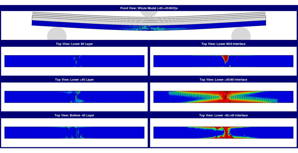
192

193 5 6 Figure A.5: FE simulations of failure progression the type-a laminate specimens (-45 8 /+45 8 /9 8 / 8 ) s. Contour plots show damage extent. 176

194 Load [kn] Type-B (64-ply, width = 12.7 mm) Laminate Test-1 Test-2 Test-3 Simulation Center Deflection [mm] SDV_DAMAGESTATE (Avg: 75%) +1.e e e e e e 1 +5.e e e e e e 2 +.e+ CSDMG General_Contact_Domain +1.e e e e e e 1 +5.e e e e e e 2 +.e

195

196 6 Figure A.6: FE simulations of failure progression the type-b laminate specimens (+45 8 /-45 8 / 8 /9 8 ) s. Contour plots show damage extent. was provided as CSDMG. Both damage variables range from to 1, where (blue in the contour plots) denotes an elastic, pre-damage state and 1 (red in the contour plots) denotes a cracked state. Elements that reach the fully cracked state of intra-lamina failure (SDV DAMAGESTATE=1) will be deleted so that the cracks are also visible in the results of the FE simulations. Good agreement in stiffness and failure loads of load-displacement responses can be seen between the FE simulations and the experiment data, for both laminates. The stable responses provided by the FE simulations suggest that the mass scaling chosen is appropriate for simulating quasi-static tests. As shown in Figure A.5, the failure progression observed in the experiments is captured by the FE simulations for the type-a laminates. The initial failure is matrix cracking in bottom -45 layer, which further induces delamination at the interface with the adjacent +45 layer. As those matrix cracks extend in the width direction and more cracks develop in the -45 layer, matrix cracks also initiate in +45 and 9 layers. The large load drop of the load-displacement response, which indicates a loss of stiffness, is caused by the development of through-width matrix cracks in those three layers and a large delamination at the lower 9/ interface. The noise seen in results at the lower +45/9 interface may be caused by the mismatch of structured meshes in the adjacent +45, 9 layers. The failure progression is also well captured by the FE simulations for the type-b laminates, as shown in Figure A.6. In experiments, strain concentration is initially seen near the center location of middle 9 layer closed to its interface with lower layer, as shown in Figure A.4. The FE simulations predict damage initiation at 179