CONTROL SYSTEMS LECTURE NOTES B.TECH (II YEAR II SEM) ( ) Prepared by: Mrs.P.ANITHA, Associate Professor Mr.V.KIRAN KUMAR, Assistant Professor

Transcription

1 LECTURE NOTES B.TECH (II YEAR II SEM) ( ) Prepared by: Mrs.P.ANITHA, Associate Professor Mr.V.KIRAN KUMAR, Assistant Professor Department of Electronics and Communication Engineering MALLA REDDY COLLEGE OF ENGINEERING & TECHNOLOGY (Autonomous Institution UGC, Govt. of India) Recognized under 2(f) and 12 (B) of UGC ACT 1956 (Affiliated to JNTUH, Hyderabad, Approved by AICTE - Accredited by NBA & NAAC A Grade - ISO 9001:2015 Certified) Maisammaguda, Dhulapally (Post Via. Kompally), Secunderabad , Telangana State, India

2 MALLA REDDY COLLEGE OF ENGINEERING AND TECHNOLOGY II Year B.Tech. ECE-II Sem L T/P/D C 3 1/ - /- 3 (R15A0203) OBJECTIVES In this course it is aimed to 1. Introduce the principles and applications of control systems in everyday life. 2. The basic concepts of block diagram reduction, transfer function representation, time response and time domain analysis, solutions to time invariant systems and also deals with the different aspects of stability analysis of systems in frequency domain and time domain. UNIT - I: Introduction: Concept of control system, Classification of control systems - Open loop and closed loop control systems, Differences, Examples of control systems- Effects of feedback, Feedback Characteristics. Transfer Function Representation: Block diagram algebra, Determining the Transfer function from Block Diagrams, Signal flow graphs(sfg) - Reduction using Mason s gain formula- Transfer function of SFG s. UNIT - II: Time Response Analysis: Standard test signals, Time response of first order systems, Characteristic Equation of Feedback control systems, Transient response of second order systems - Time domain specifications, Steady state response, Steady state errors and error constants, PID controllers: Effects of proportional derivative, proportional integral systems on steady state error. UNIT - III: Stability Analysis in S-Domain: The concept of stability Routh-Hurwitz s stability criterion qualitative stability and conditional stability Limitations of Routh-Hurwitz s stability. Root Locus Technique: Concept of root locus - Construction of root locus. UNIT - IV: Frequency Response Analysis: Introduction, Frequency domain specifications, Bode plot diagrams-determination of Phase margin and Gain margin, Stability analysis from Bode plots, Polar plots, Nyquist plots. UNIT - V: State Space Analysis of Continuous Systems: Concepts of state, state variables and state model, Derivation of state models from block diagrams, Diagonalization, Solving the time invariant state equations, State Transition Matrix and it s properties, Concepts of Controllability and observability. TEXT BOOKS: 1. Control Systems Engineering - I. J. Nagrath and M. Gopal, New Age International (P) Limited, Publishers. 2. Control Systems - A. Ananad Kumar, PHI. 3. Control Systems Engineering by A. Nagoor Kani, RBA Publications.

3 REFERENCE BOOKS: 1. Control Systems Theory and Applications - S. K. Bhattacharya, Pearson. 2. Control Systems Engineering - S. Palani, TMH. 3. Control Systems - N. K. Sinha, New Age International (P) Limited Publishers. 4. Control Systems by S.Hasan Saeed, KATSON BOOKS. 5. Solutions and Problems of Control Systems by A.K. Jairath, CBS Publishers. OUTCOMES After going through this course the student gets 1. A thorough knowledge on open loop and closed loop control systems, concept of feedback in control systems. 2. Transfer function representation through block diagram algebra and signal flow graphs. 3. Time response analysis of different ordered systems through their characteristic equation. 4. Time domain specifications, stability analysis of control systems in s-domain through R-H criteria. 5. Root locus techniques, frequency response analysis through Bode diagrams, Nyquist, Polar plots. 6. The basics of state space analysis, design of lag, lead compensators, with which he/she can able to apply the above conceptual things to real world electrical and electronics problems and applications.

4 UNIT-I INTRODUCTION A control system manages commands, directs or regulates the behavior of other devices or systems using control loops. It can range from a single home heating controller using a thermostat controlling a domestic boiler to large Industrial control systems which are used for controlling processes or machines. A control system is a system, which provides the desired response by controlling the output. The following figure shows the simple block diagram of a control system. Examples Traffic lights control system, washing machine Traffic lights control system is an example of control system. Here, a sequence of input signal is applied to this control system and the output is one of the three lights that will be on for some duration of time. During this time, the other two lights will be off. Based on the traffic study at a particular junction, the on and off times of the lights can be determined. Accordingly, the input signal controls the output. So, the traffic lights control system operates on time basis. CLASSIFICATION OF Based on some parameters, we can classify the control systems into the following ways. Continuous time and Discrete-time Control Systems Control Systems can be classified as continuous time control systems and discrete time control systems based on the type of the signal used. In continuous time control systems, all the signals are continuous in time. But, in discrete time control systems, there exists one or more discrete time signals. SISO and MIMO Control Systems Control Systems can be classified as SISO control systems and MIMO control systems based on the number of inputs and outputs present.

5 SISO (Single Input and Single Output) control systems have one input and one output. Whereas, MIMO (Multiple Inputs and Multiple Outputs) control systems have more than one input and more than one output. Open Loop and Closed Loop Control Systems Control Systems can be classified as open loop control systems and closed loop control systems based on the feedback path. In open loop control systems, output is not fed-back to the input. So, the control action is independent of the desired output. The following figure shows the block diagram of the open loop control system. Here, an input is applied to a controller and it produces an actuating signal or controlling signal. This signal is given as an input to a plant or process which is to be controlled. So, the plant produces an output, which is controlled. The traffic lights control system which we discussed earlier is an example of an open loop control system. In closed loop control systems, output is fed back to the input. So, the control action is dependent on the desired output. The following figure shows the block diagram of negative feedback closed loop control system.

6 The error detector produces an error signal, which is the difference between the input and the feedback signal. This feedback signal is obtained from the block (feedback elements) by considering the output of the overall system as an input to this block. Instead of the direct input, the error signal is applied as an input to a controller. So, the controller produces an actuating signal which controls the plant. In this combination, the output of the control system is adjusted automatically till we get the desired response. Hence, the closed loop control systems are also called the automatic control systems. Traffic lights control system having sensor at the input is an example of a closed loop control system. The differences between the open loop and the closed loop control systems are mentioned in the following table. If either the output or some part of the output is returned to the input side and utilized as part of the system input, then it is known as feedback. Feedback plays an important role in order to improve the performance of the control systems. In this chapter, let us discuss the types of feedback & effects of feedback. Types of Feedback There are two types of feedback Positive feedback Negative feedback

7 Positive Feedback The positive feedback adds the reference input, R(s)R(s) and feedback output. The following figure shows the block diagram of positive feedback control system he concept of transfer function will be discussed in later chapters. For the time being, consider the transfer function of positive feedback control system is, Where, T is the transfer function or overall gain of positive feedback control system. G is the open loop gain, which is function of frequency. H is the gain of feedback path, which is function of frequency. Negative Feedback Negative feedback reduces the error between the reference input, R(s)R(s) and system output. The following figure shows the block diagram of the negative feedback control system.

8 Transfer function of negative feedback control system is, Where, T is the transfer function or overall gain of negative feedback control system. G is the open loop gain, which is function of frequency. H is the gain of feedback path, which is function of frequency. The derivation of the above transfer function is present in later chapters. EFFECTS OF FEEDBACK Let us now understand the effects of feedback. Effect of Feedback on Overall Gain From Equation 2, we can say that the overall gain of negative feedback closed loop control system is the ratio of 'G' and (1+GH). So, the overall gain may increase or decrease depending on the value of (1+GH). If the value of (1+GH) is less than 1, then the overall gain increases. In this case, 'GH' value is negative because the gain of the feedback path is negative. If the value of (1+GH) is greater than 1, then the overall gain decreases. In this case, 'GH' value is positive because the gain of the feedback path is positive. In general, 'G' and 'H' are functions of frequency. So, the feedback will increase the overall gain of the system in one frequency range and decrease in the other frequency range. Effect of Feedback on Sensitivity Sensitivity of the overall gain of negative feedback closed loop control system (T) to the variation in open loop gain (G) is defined as

9 So, we got the sensitivity of the overall gain of closed loop control system as the reciprocal of (1+GH). So, Sensitivity may increase or decrease depending on the value of (1+GH). If the value of (1+GH) is less than 1, then sensitivity increases. In this case, 'GH' value is negative because the gain of feedback path is negative. If the value of (1+GH) is greater than 1, then sensitivity decreases. In this case, 'GH' value is positive because the gain of feedback path is positive. In general, 'G' and 'H' are functions of frequency. So, feedback will increase the sensitivity of the system gain in one frequency range and decrease in the other frequency range. Therefore, we have to choose the values of 'GH' in such a way that the system is insensitive or less sensitive to parameter variations. Effect of Feedback on Stability A system is said to be stable, if its output is under control. Otherwise, it is said to be unstable. In Equation 2, if the denominator value is zero (i.e., GH = -1), then the output of the control system will be infinite. So, the control system becomes unstable. Therefore, we have to properly choose the feedback in order to make the control system stable. Effect of Feedback on Noise To know the effect of feedback on noise, let us compare the transfer function relations with and without feedback due to noise signal alone. Consider an open loop control system with noise signal as shown below.

10

11 The control systems can be represented with a set of mathematical equations known as mathematical model. These models are useful for analysis and design of control systems. Analysis of control system means finding the output when we know the input and mathematical model. Design of control system means finding the mathematical model when we know the input and the output. The following mathematical models are mostly used. Differential equation model Transfer function model State space model TRANSFER FUNCTION REPRESENTATION Block Diagrams Block diagrams consist of a single block or a combination of blocks. These are used to represent the control systems in pictorial form. Basic Elements of Block Diagram The basic elements of a block diagram are a block, the summing point and the take-off point. Let us consider the block diagram of a closed loop control system as shown in the following figure to identify these elements.

12 The above block diagram consists of two blocks having transfer functions G(s) and H(s). It is also having one summing point and one take-off point. Arrows indicate the direction of the flow of signals. Let us now discuss these elements one by one. Block The transfer function of a component is represented by a block. Block has single input and single output. The following figure shows a block having input X(s), output Y(s) and the transfer function G(s). Summing Point The summing point is represented with a circle having cross (X) inside it. It has two or more inputs and single output. It produces the algebraic sum of the inputs. It also performs the summation or subtraction or combination of summation and subtraction of the inputs based on the polarity of the inputs. Let us see these three operations one by one. The following figure shows the summing point with two inputs (A, B) and one output (Y). Here, the inputs A and B have a positive sign. So, the summing point produces the output, Y as sum of A and B i.e. = A + B. The following figure shows the summing point with two inputs (A, B) and one output (Y). Here, the inputs A and B are having opposite signs, i.e., A is having positive sign and B is having negative sign. So, the summing point produces the output Y as the difference of A and B i.e

13 Y = A + (-B) = A - B. The following figure shows the summing point with three inputs (A, B, C) and one output (Y). Here, the inputs A and B are having positive signs and C is having a negative sign. So, the summing point produces the output Y as Y = A + B + ( C) = A + B C. Take-off Point The take-off point is a point from which the same input signal can be passed through more than one branch. That means with the help of take-off point, we can apply the same input to one or more blocks, summing points.in the following figure, the take-off point is used to connect the same input, R(s) to two more blocks.

14 In the following figure, the take-off point is used to connect the output C(s), as one of the inputs to the summing point. Block diagram algebra is nothing but the algebra involved with the basic elements of the block diagram. This algebra deals with the pictorial representation of algebraic equations. Basic Connections for Blocks There are three basic types of connections between two blocks. Series Connection Series connection is also called cascade connection. In the following figure, two blocks having transfer functions G1(s)G1(s) and G2(s)G2(s) are connected in series.

15 That means we can represent the series connection of two blocks with a single block. The transfer function of this single block is the product of the transfer functions of those two blocks. The equivalent block diagram is shown below. Similarly, you can represent series connection of n blocks with a single block. The transfer function of this single block is the product of the transfer functions of all those n blocks. Parallel Connection The blocks which are connected in parallel will have the same input. In the following figure, two blocks having transfer functions G1(s)G1(s) and G2(s)G2(s) are connected in parallel. The outputs of these two blocks are connected to the summing point.

16 That means we can represent the parallel connection of two blocks with a single block. The transfer function of this single block is the sum of the transfer functions of those two blocks. The equivalent block diagram is shown below. Similarly, you can represent parallel connection of n blocks with a single block. The transfer function of this single block is the algebraic sum of the transfer functions of all those n blocks. Feedback Connection As we discussed in previous chapters, there are two types of feedback positive feedback and negative feedback. The following figure shows negative feedback control system. Here, two blocks having transfer functions G(s)G(s) and H(s)H(s) form a closed loop.

17 Therefore, the negative feedback closed loop transfer function is : This means we can represent the negative feedback connection of two blocks with a single block. The transfer function of this single block is the closed loop transfer function of the negative feedback. The equivalent block diagram is shown below.

18 Similarly, you can represent the positive feedback connection of two blocks with a single block. The transfer function of this single block is the closed loop transfer function of the positive feedback, i.e., Block Diagram Algebra for Summing Points There are two possibilities of shifting summing points with respect to blocks Shifting summing point after the block Shifting summing point before the block Let us now see what kind of arrangements need to be done in the above two cases one by one. Shifting the Summing Point before a Block to after a Block Consider the block diagram shown in the following figure. Here, the summing point is present before the block. The output of Summing point is

19 Compare Equation 1 and Equation 2. The first term G(s)R(s) G(s)R(s) is same in both the equations. But, there is difference in the second term. In order to get the second term also same, we require one more block G(s)G(s). It is having the input X(s)X(s) and the output of this block is given as input to summing point instead of X(s)X(s). This block diagram is shown in the following figure.

20 Compare Equation 3 and Equation 4, The first term G(s) R(s) is same in both equations. But, there is difference in the second term. In order to get the second term also same, we require one more block 1/G(s). It is having the input X(s) and the output of this block is given as input to summing point instead of X(s). This block diagram is shown in the following figure.

21 Block Diagram Algebra for Take-off Points There are two possibilities of shifting the take-off points with respect to blocks Shifting take-off point after the block Shifting take-off point before the block Let us now see what kind of arrangements is to be done in the above two cases, one by one. Shifting a Take-off Point form a Position before a Block to a position after the Block Consider the block diagram shown in the following figure. In this case, the take-off point is present before the block. When you shift the take-off point after the block, the output Y(s) will be same. But, there is difference in X(s) value. So, in order to get the same X(s) value, we require one more block 1/G(s). It is having the input Y(s) and the output is X(s) this block diagram is shown in the following figure.

22 Shifting Take-off Point from a Position after a Block to a position before the Block Consider the block diagram shown in the following figure. Here, the take-off point is present after the block. When you shift the take-off point before the block, the output Y(s) will be same. But, there is difference in X(s) value. So, in order to get same X(s) value, we require one more block G(s) It is having the input R(s) and the output is X(s). This block diagram is shown in the following figure. The concepts discussed in the previous chapter are helpful for reducing (simplifying) the block diagrams. Block Diagram Reduction Rules Follow these rules for simplifying (reducing) the block diagram, which is having many blocks, summing points and take-off points. Rule 1 Check for the blocks connected in series and simplify. Rule 2 Check for the blocks connected in parallel and simplify.

23 Rule 3 Check for the blocks connected in feedback loop and simplify. Rule 4 If there is difficulty with take-off point while simplifying, shift it towards right. Rule 5 If there is difficulty with summing point while simplifying, shift it towards left. Rule 6 Repeat the above steps till you get the simplified form, i.e., single block. Note The transfer function present in this single block is the transfer function of the overall block diagram. Example Consider the block diagram shown in the following figure. Let us simplify (reduce) this block diagram using the block diagram reduction rules.

24

25 Note Follow these steps in order to calculate the transfer function of the block diagram having multiple inputs. Step 1 Find the transfer function of block diagram by considering one input at a time and make the remaining inputs as zero. Step 2 Repeat step 1 for remaining inputs. Step 3 Get the overall transfer function by adding all those transfer functions. The block diagram reduction process takes more time for complicated systems because; we have to draw the (partially simplified) block diagram after each step. So, to overcome this drawback, use signal flow graphs (representation).

26 Block Diagram Reduction- Summary

27

28 Example-1:

29

30 Example-2:

31 Signal flow graph is a graphical representation of algebraic equations. In this chapter, let us discuss the basic concepts related signal flow graph and also learn how to draw signal flow graphs. Basic Elements of Signal Flow Graph Nodes and branches are the basic elements of signal flow graph. Node Node is a point which represents either a variable or a signal. There are three types of nodes input node, output node and mixed node. Input Node It is a node, which has only outgoing branches. Output Node It is a node, which has only incoming branches. Mixed Node It is a node, which has both incoming and outgoing branches. Example Let us consider the following signal flow graph to identify these nodes. Branch Branch is a line segment which joins two nodes. It has both gain and direction. For example, there are four branches in the above signal flow graph. These branches have gains of a, b, c and -d.

32 Construction of Signal Flow Graph Let us construct a signal flow graph by considering the following algebraic equations

33

34 Conversion of Block Diagrams into Signal Flow Graphs Follow these steps for converting a block diagram into its equivalent signal flow graph. Represent all the signals, variables, summing points and take-off points of block diagram as nodes in signal flow graph. Represent the blocks of block diagram as branches in signal flow graph. Represent the transfer functions inside the blocks of block diagram asgains of the branches in signal flow graph. Connect the nodes as per the block diagram. If there is connection between two nodes (but there is no block in between), then represent the gain of the branch as one. For example, between summing points, between summing point and takeoff point, between input and summing point, between take-off point and output. Example Let us convert the following block diagram into its equivalent signal flow graph. Represent the input signal R(s) and output signal C(s) of block diagram as input node R(s) and output node C(s) of signal flow graph. Just for reference, the remaining nodes (y1 to y9) are labelled in the block diagram. There are nine nodes other than input and output nodes. That is four nodes for four summing points, four nodes for four take-off points and one node for the variable between blocks G1and G2.

35 The following figure shows the equivalent signal flow graph. Let us now discuss the Mason s Gain Formula. Suppose there are N forward paths in a signal flow graph. The gain between the input and the output nodes of a signal flow graph is nothing but the transfer function of the system. It can be calculated by using Mason s gain formula. Mason s gain formula is Where, C(s) is the output node R(s) is the input node T is the transfer function or gain between R(s) and C(s) Pi is the i th forward path gain Δ=1 (sum of all individual loop gains) +(sum of gain products of all possible two nontouching loops) (sum of gain products of all possible three nontouching loops) +. Δi is obtained from Δ by removing the loops which are touching the i th forward path.

36 Consider the following signal flow graph in order to understand the basic terminology involved here. Loop The path that starts from one node and ends at the same node is known as a loop. Hence, it is a closed path.

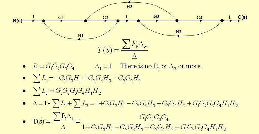
37 Calculation of Transfer Function using Mason s Gain Formula Let us consider the same signal flow graph for finding transfer function. Number of forward paths, N = 2. First forward path is - y1 y2 y3 y4 y5 y6. First forward path gain, p1=abcde Second forward path is - y1 y2 y3 y5 y6 Second forward path gain, p2=abge Number of individual loops, L = 5. Number of two non-touching loops = 2. First non-touching loops pair is - y2 y3 y2, y4 y5 y4.

38 Gain product of first non-touching loops pair l1l4=bjdi Second non-touching loops pair is - y2 y3 y2, y5 y5. Gain product of second non-touching loops pair is l1l5=bjf Higher number of (more than two) non-touching loops are not present in this signal flow graph.we know,

39

40

41 Example-1:

42 Example-2:

43 Example-3:

44 UNIT-II TIME RESPONSE ANALYSIS We can analyze the response of the control systems in both the time domain and the frequency domain. We will discuss frequency response analysis of control systems in later chapters. Let us now discuss about the time response analysis of control systems. What is Time Response? If the output of control system for an input varies with respect to time, then it is called the time response of the control system. The time response consists of two parts. Transient response Steady state response The response of control system in time domain is shown in the following figure.

45 Where, ctr(t) is the transient response css(t) is the steady state response Transient Response After applying input to the control system, output takes certain time to reach steady state. So, the output will be in transient state till it goes to a steady state. Therefore, the response of the control system during the transient state is known as transient response. The transient response will be zero for large values of t. Ideally, this value of t is infinity and practically, it is five times constant. Mathematically, we can write it as

46 Steady state Response The part of the time response that remains even after the transient response has zero value for large values of t is known as steady state response. This means, the transient response will be zero even during the steady state. Example Let us find the transient and steady state terms of the time response of the control system Here, the second term will be zero as t denotes infinity. So, this is the transient term. And the first term 10 remains even as t approaches infinity. So, this is the steady state term. Standard Test Signals The standard test signals are impulse, step, ramp and parabolic. These signals are used to know the performance of the control systems using time response of the output. Unit Impulse Signal A unit impulse signal, δ(t) is defined as The unit Impulse Signal So, the unit impulse signal exists only at t is equal to zero. The area of this signal under small

47 interval of time around t is equal to zero is one. The value of unit impulse signal is zero for all other values of t. Unit Step Signal A unit step signal, u(t) is defined as Following figure shows unit step signal. So, the unit step signal exists for all positive values of t including zero. And its value is one during this interval. The value of the unit step signal is zero for all negative values of t. Unit Ramp Signal A unit ramp signal, r (t) is defined as

48 So, the unit ramp signal exists for all positive values of t including zero. And its value increases linearly with respect to t during this interval. The value of unit ramp signal is zero for all negative values of t. Unit Parabolic Signal A unit parabolic signal, p(t) is defined as,

49 So, the unit parabolic signal exists for all the positive values of t including zero. And its value increases non-linearly with respect to t during this interval. The value of the unit parabolic signal is zero for all the negative values of t. In this chapter, let us discuss the time response of the first order system. Consider the following block diagram of the closed loop control system. Here, an open loop transfer function, 1/sT is connected with a unity negative feedback. The power of S is one in the denominator of the Transfer function. Hence, it is a First order System.

50 Impulse Response of First Order System Consider the unit impulse signal as an input to the first order system. So, r(t)=δ(t) Apply Laplace transform on both the sides. R(s) =1 Rearrange the above equation in one of the standard forms of Laplace transforms.

51 Applying Inverse Laplace Transform on both the sides, The unit impulse response is shown in the following figure. The unit impulse response, c(t) is an exponential decaying signal for positive values of t and it is zero for negative values of t. Step Response of First Order System Consider the unit step signal as an input to first order system. So, r(t)=u(t)

52 On both the sides, the denominator term is the same. So, they will get cancelled by each other. Hence, equate the numerator terms. 1=A(sT+1)+Bs By equating the constant terms on both the sides, you will get A = 1. Substitute, A = 1 and equate the coefficient of the s terms on both the sides. 0=T+B B= T Substitute, A = 1 and B = T in partial fraction expansion of C(s) Apply inverse Laplace transform on both the sides.

53 The unit step response, c(t) has both the transient and the steady state terms. The transient term in the unit step response is - The steady state term in the unit step response is The following figure shows the unit step response The value of the unit step response, c(t) is zero at t = 0 and for all negative values of t. It is gradually increasing from zero value and finally reaches to one in steady state. So, the steady state value depends on the magnitude of the input. Ramp Response of First Order System Consider the unit ramp signal as an input to the first order system. So,r(t)=t u(t) Apply Laplace transform on both the sides.

54 On both the sides, the denominator term is the same. So, they will get cancelled by each other. Hence, equate the numerator terms. By equating the constant terms on both the sides, you will get A = 1. Substitute, A = 1 and equate the coefficient of the s terms on both the sides. 0=T+B B= T Similarly, substitute B = T and equate the coefficient of s 2 terms on both the sides. You will get C=T 2 Substitute A = 1, B = T and C=T 2 in the partial fraction expansion of C(s). Apply inverse Laplace transform on both the sides. The unit ramp response, c(t) has both the transient and the steady state terms. The transient term in the unit ramp response is

55 The steady state term in the unit ramp response is The figure below is the unit ramp response: The unit ramp response, c(t) follows the unit ramp input signal for all positive values of t. But, there is a deviation of T units from the input signal. Parabolic Response of First Order System Consider the unit parabolic signal as an input to the first order system. \

56 Apply inverse Laplace transform on both the sides. The unit parabolic response, c(t) has both the transient and the steady state terms. The transient term in the unit parabolic response is The steady state term in the unit parabolic response is From these responses, we can conclude that the first order control systems are not stable with the ramp and parabolic inputs because these responses go on increasing even at infinite amount of time. The first order control systems are stable with impulse and step inputs because these responses have bounded output. But, the impulse response doesn t have steady state term. So, the step signal is widely used in the time domain for analyzing the control systems from their responses.in this chapter, let us discuss the time response of second order system. Consider the following block diagram of closed loop control system. Here, an open loop transfer function, ωn 2 / s(s+2δωn) is connected with a unity negative feedback.

57 The power of s is two in the denominator term. Hence, the above transfer function is of the second order and the system is said to be the second order system. The characteristic equation is - b

58 The two roots are imaginary when δ = 0. The two roots are real and equal when δ = 1. The two roots are real but not equal when δ > 1. The two roots are complex conjugate when 0 < δ < 1. We can write C(s) equation as, Where, C(s) is the Laplace transform of the output signal, c(t) R(s) is the Laplace transform of the input signal, r(t) ωn is the natural frequency δ is the damping ratio. Follow these steps to get the response (output) of the second order system in the time domain. Step Response of Second Order System Consider the unit step signal as an input to the second order system. Laplace transform of the unit step signal is, The Transfer function of the Second order closed loop control system is given by:

59

60

61

62 So, the unit step response of the second order system is having damped oscillations (decreasing amplitude) when δ lies between zero and one. Case 4: δ > 1 We can modify the denominator term of the transfer function as follows

63 Since it is over damped, the unit step response of the second order system when δ > 1 will never reach step input in the steady state. Impulse Response of Second Orde r System The impulse response of the second order system can be obtained by using any one of these two methods. Follow the procedure involved while deriving step response by considering the value of R(s) as 1 instead of 1/s. Do the differentiation of the step response. The following table shows the impulse response of the second order system for 4 cases of the damping ratio.

64 In this chapter, let us discuss the time domain specifications of the second order system. The step response of the second order system for the underdamped case is shown in the following figure.

65 All the time domain specifications are represented in this figure. The response up to the settling time is known as transient response and the response after the settling time is known as steady state response. Delay Time It is the time required for the response to reach half of its final value from the zero instant. It is denoted by tdtd. Consider the step response of the second order system for t 0, when δ lies between zero and one. Rise Time It is the time required for the response to rise from 0% to 100% of its final value. This is applicable for the under-damped systems. For the over-damped systems, consider the duration from 10% to 90% of the final value. Rise time is denoted by tr. At t = t1 = 0, c(t) = 0. We know that the final value of the step response is one.therefore, at t=t2, the value of step response is one. Substitute, these values in the following equation.

66 From above equation, we can conclude that the rise time tr and the damped frequency ωd are inversely proportional to each other. Peak Time It is the time required for the response to reach the peak value for the first time. It is denoted by tp. At t=tp the first derivate of the response is zero. We know the step response of second order system for under-damped case is

67 From the above equation, we can conclude that the peak time tp and the damped frequency ωd are inversely proportional to each other. Peak Overshoot Peak overshoot Mp is defined as the deviation of the response at peak time from the final value of response. It is also called the maximum overshoot. Mathematically, we can write it as Mp=c(tp) c( ) Where,c(tp) is the peak value of the response, c( ) is the final (steady state) value of the response.

68 At t=tp, the response c(t) is -

69 From the above equation, we can conclude that the percentage of peak overshoot %Mp will decrease if the damping ratio δ increases. Settling time It is the time required for the response to reach the steady state and stay within the specified tolerance bands around the final value. In general, the tolerance bands are 2% and 5%. The settling time is denoted by ts. The settling time for 5% tolerance band is The settling time for 2% tolerance band is Where, τ is the time constant and is equal to 1/δωn. Both the settling time ts and the time constant τ are inversely proportional to the damping ratio δ. Both the settling time ts and the time constant τ are independent of the system gain. That means even the system gain changes, the settling time ts and time constant τ will never change. Example Let us now find the time domain specifications of a control system having the closed loop transfer function when the unit step signal is applied as an input to this control system. We know that the standard form of the transfer function of the second order closed loop control system as By equating these two transfer functions, we will get the un-damped natural frequency ωn as 2 rad/sec and the damping ratio δ as 0.5. We know the formula for damped frequency ωd as

70 Substitute the above necessary values in the formula of each time domain specification and simplify in order to get the values of time domain specifications for given transfer function. The following table shows the formulae of time domain specifications, substitution of necessary values and the final values

71 The deviation of the output of control system from desired response during steady state is known as steady state error. It is represented as ess. We can find steady state error using the final value theorem as follows. Where, E(s) is the Laplace transform of the error signal, e(t) Let us discuss how to find steady state errors for unity feedback and non-unity feedback control systems one by one.

72 Steady State Errors for Unity Feedback Systems Consider the following block diagram of closed loop control system, which is having unity negative feedback.

73 The following table shows the steady state errors and the error constants for standard input signals like unit step, unit ramp & unit parabolic signals. Where, Kp, Kv and Ka are position error constant, velocity error constant and acceleration error constant respectively.

74 Note If any of the above input signals has the amplitude other than unity, then multiply corresponding steady state error with that amplitude. Note We can t define the steady state error for the unit impulse signal because, it exists only at origin. So, we can t compare the impulse response with the unit impulse input as t denotes infinity We will get the overall steady state error, by adding the above three steady state errors. ess = ess1+ess2+ess3 ess=0+0+1=1 ess=0+0+1=1 Therefore, we got the steady state error ess as 1 for this example. Steady State Errors for Non-Unity Feedback Systems Consider the following block diagram of closed loop control system, which is having non unity negative feedback.

75 We can find the steady state errors only for the unity feedback systems. So, we have to convert the non-unity feedback system into unity feedback system. For this, include one unity positive feedback path and one unity negative feedback path in the above block diagram. The new block diagram looks like as shown below. Simplify the above block diagram by keeping the unity negative feedback as it is. The following is the simplified block diagram

76 This block diagram resembles the block diagram of the unity negative feedback closed loop control system. Here, the single block is having the transfer function G(s) / [ 1+G(s)H(s) G(s)] instead of G(s).You can now calculate the steady state errors by using steady state error formula given for the unity negative feedback systems. Note It is meaningless to find the steady state errors for unstable closed loop systems. So, we have to calculate the steady state errors only for closed loop stable systems. This means we need to check whether the control system is stable or not before finding the steady state errors. In the next chapter, we will discuss the concepts-related stability. The various types of controllers are used to improve the performance of control systems. In this chapter, we will discuss the basic controllers such as the proportional, the derivative and the integral controllers. Proportional Controller The proportional controller produces an output, which is proportional to error signal. Therefore, the transfer function of the proportional controller is KPKP.

77 Where, U(s) is the Laplace transform of the actuating signal u(t) E(s) is the Laplace transform of the error signal e(t) KP is the proportionality constant The block diagram of the unity negative feedback closed loop control system along with the proportional controller is shown in the following figure. Derivative Controller The derivative controller produces an output, which is derivative of the error signal. Therefore, the transfer function of the derivative controller is KDs. Where, KD is the derivative constant. The block diagram of the unity negative feedback closed loop control system along with the derivative controller is shown in the following figure.

78 The derivative controller is used to make the unstable control system into a stable one. Integral Controller The integral controller produces an output, which is integral of the error signal. Where, KIKI is the integral constant. The block diagram of the unity negative feedback closed loop control system along with the integral controller is shown in the following figure.

79 The integral controller is used to decrease the steady state error. Let us now discuss about the combination of basic controllers. Proportional Derivative (PD) Controller The proportional derivative controller produces an output, which is the combination of the outputs of proportional and derivative controllers. Therefore, the transfer function of the proportional derivative controller is KP+KDs. The block diagram of the unity negative feedback closed loop control system along with the proportional derivative controller is shown in the following figure. The proportional derivative controller is used to improve the stability of control system without affecting the steady state error. Proportional Integral (PI) Controller The proportional integral controller produces an output, which is the combination of outputs of the proportional and integral controllers.

80 The block diagram of the unity negative feedback closed loop control system along with the proportional integral controller is shown in the following figure. The proportional integral controller is used to decrease the steady state error without affecting the stability of the control system. Proportional I ntegral Derivative (PID) Controller The proportional integral derivative controller produces an output, which is the combination of the outputs of proportional, integral and derivative controllers.

81 The block diagram of the unity negative feedback closed loop control system along with the proportional integral derivative controller is shown in the following figure.

82 UNIT - III STABILITY ANALYSIS IN S-DOMAIN Stability is an important concept. In this chapter, let us discuss the stability of system and types of systems based on stability. What is Stability? A system is said to be stable, if its output is under control. Otherwise, it is said to be unstable. A stable system produces a bounded output for a given bounded input. The following figure shows the response of a stable system. This is the response of first order control system for unit step input. This response has the values between 0 and 1. So, it is bounded output. We know that the unit step signal has the value of one for all positive values of t including zero. So, it is bounded input. Therefore, the first order control system is stable since both the input and the output are bounded. Types of Systems based on Stability We can classify the systems based on stability as follows. Absolutely stable system Conditionally stable system Marginally stable system

83 Absolutely Stable System If the system is stable for all the range of system component values, then it is known as the absolutely stable system. The open loop control system is absolutely stable if all the poles of the open loop transfer function present in left half of s plane. Similarly, the closed loop control system is absolutely stable if all the poles of the closed loop transfer function present in the left half of the s plane. Conditionally Stable System If the system is stable for a certain range of system component values, then it is known as conditionally stable system. Marginally Stable System If the system is stable by producing an output signal with constant amplitude and constant frequency of oscillations for bounded input, then it is known as marginally stable system. The open loop control system is marginally stable if any two poles of the open loop transfer function is present on the imaginary axis. Similarly, the closed loop control system is marginally stable if any two poles of the closed loop transfer function is present on the imaginary axis. n this chapter, let us discuss the stability analysis in the s domain using the RouthHurwitz stability criterion. In this criterion, we require the characteristic equation to find the stability of the closed loop control systems. Routh-Hurwitz Stability Criterion Routh-Hurwitz stability criterion is having one necessary condition and one sufficient condition for stability. If any control system doesn t satisfy the necessary condition, then we can say that the control system is unstable. But, if the control system satisfies the necessary condition, then it may or may not be stable. So, the sufficient condition is helpful for knowing whether the control system is stable or not. Necessary Condition for Routh-Hurwitz Stability The necessary condition is that the coefficients of the characteristic polynomial should be positive. This implies that all the roots of the characteristic equation should have negative real parts. Consider the characteristic equation of the order n is -

84 Note that, there should not be any term missing in the n th order characteristic equation. This means that the n th order characteristic equation should not have any coefficient that is of zero value. Sufficient Condition for Routh-Hurwitz Stability The sufficient condition is that all the elements of the first column of the Routh array should have the same sign. This means that all the elements of the first column of the Routh array should be either positive or negative. Routh Array Method If all the roots of the characteristic equation exist to the left half of the s plane, then the control system is stable. If at least one root of the characteristic equation exists to the right half of the s plane, then the control system is unstable. So, we have to find the roots of the characteristic equation to know whether the control system is stable or unstable. But, it is difficult to find the roots of the characteristic equation as order increases. So, to overcome this problem there we have the Routh array method. In this method, there is no need to calculate the roots of the characteristic equation. First formulate the Routh table and find the number of the sign changes in the first column of the Routh table. The number of sign changes in the first column of the Routh table gives the number of roots of characteristic equation that exist in the right half of the s plane and the control system is unstable. Follow this procedure for forming the Routh table. Fill the first two rows of the Routh array with the coefficients of the characteristic polynomial as mentioned in the table below. Start with the coefficient of sn and continue up to the coefficient of s0. Fill the remaining rows of the Routh array with the elements as mentioned in the table below. Continue this process till you get the first column element of row s0s0 is an. Here, an is the coefficient of s0 in the characteristic polynomial. Note If any row elements of the Routh table have some common factor, then you can divide the row elements with that factor for the simplification will be easy. The following table shows the Routh array of the n th order characteristic polynomial.

85 Example Let us find the stability of the control system having characteristic equation, Step 1 Verify the necessary condition for the Routh-Hurwitz stability. All the coefficients of the characteristic polynomial, are positive. So, the control system satisfies the necessary condition. Step 2 Form the Routh array for the given characteristic polynomial.

86 Step 3 Verify the sufficient condition for the Routh-Hurwitz stability. All the elements of the first column of the Routh array are positive. There is no sign change in the first column of the Routh array. So, the control system is stable. Special Cases of Routh Array We may come across two types of situations, while forming the Routh table. It is difficult to complete the Routh table from these two situations. The two special cases are The first element of any row of the Routh s array is zero. All the elements of any row of the Routh s array are zero. Let us now discuss how to overcome the difficulty in these two cases, one by one. First Element of any row of the Routh s array is zero If any row of the Routh s array contains only the first element as zero and at least one of the remaining elements have non-zero value, then replace the first element with a small positive integer, ϵ. And then continue the process of completing the Routh s table. Now, find the number of sign changes in the first column of the Routh s table by substituting ϵϵ tends to zero.

87 Example Let us find the stability of the control system having characteristic equation, Step 1 Verify the necessary condition for the Routh-Hurwitz stability. All the coefficients of the characteristic polynomial, necessary condition. are positive. So, the control system satisfied the Step 2 Form the Routh array for the given characteristic polynomial. The row s 3 elements have 2 as the common factor. So, all these elements are divided by 2. Special case (i) Only the first element of row s 2 is zero. So, replace it by ϵ and continue the process of completing the Routh table.

88 Step 3 Verify the sufficient condition for the Routh-Hurwitz stability. As ϵ tends to zero, the Routh table becomes like this. There are two sign changes in the first column of Routh table. Hence, the control system is unstable. All the Elements of any row of the Routh s array are zero In this case, follow these two steps Write the auxilary equation, A(s) of the row, which is just above the row of zeros. Differentiate the auxiliary equation, A(s) with respect to s. Fill the row of zeros with these coefficients.

89 Example Let us find the stability of the control system having characteristic equation, Step 1 Verify the necessary condition for the Routh-Hurwitz stability. All the coefficients of the given characteristic polynomial are positive. So, the control system satisfied the necessary condition. Step 2 Form the Routh array for the given characteristic polynomial.

90 Step 3 Verify the sufficient condition for the Routh-Hurwitz stability. There are two sign changes in the first column of Routh table. Hence, the control system is unstable. In the Routh-Hurwitz stability criterion, we can know whether the closed loop poles are in on left half of the s plane or on the right half of the s plane or on an imaginary axis. So, we can t find the nature of the control system. To overcome this limitation, there is a technique known as the root locus. Root locus Technique In the root locus diagram, we can observe the path of the closed loop poles. Hence, we can identify the nature of the control system. In this technique, we will use an open loop transfer function to know the stability of the closed loop control system.

91 Basics of Root Locus The Root locus is the locus of the roots of the characteristic equation by varying system gain K from zero to infinity. We know that, the characteristic equation of the closed loop control system is

92 From above two cases, we can conclude that the root locus branches start at open loop poles and end at open loop zeros. Angle Condition and Magnitude Condition The points on the root locus branches satisfy the angle condition. So, the angle condition is used to know whether the point exist on root locus branch or not. We can find the value of K for the points on the root locus branches by using magnitude condition. So, we can use the magnitude condition for the points, and this satisfies the angle condition. Characteristic equation of closed loop control system is The angle condition is the point at which the angle of the open loop transfer function is an odd multiple of

93 Magnitude of G(s)H(s)G(s)H(s) is The magnitude condition is that the point (which satisfied the angle condition) at which the magnitude of the open loop transfer function is one. The root locus is a graphical representation in s-domain and it is symmetrical about the real axis. Because the open loop poles and zeros exist in the s-domain having the values either as real or as complex conjugate pairs. In this chapter, let us discuss how to construct (draw) the root locus. Rules for Construction of Root Locus Follow these rules for constructing a root locus. Rule 1 Locate the open loop poles and zeros in the s plane. Rule 2 Find the number of root locus branches. We know that the root locus branches start at the open loop poles and end at open loop zeros. So, the number of root locus branches N is equal to the number of finite open loop poles P or the number of finite open loop zeros Z, whichever is greater. Mathematically, we can write the number of root locus branches N as N=P if P Z N=Z if P<Z Rule 3 Identify and draw the real axis root locus branches. If the angle of the open loop transfer function at a point is an odd multiple of 180 0, then that point is on the root locus. If odd number of the open loop poles and zeros exist to the left side of a point on the real axis, then that point is on the root locus branch. Therefore, the branch of points which satisfies this condition is the real axis of the root locus branch. Rule 4 Find the centroid and the angle of asymptotes. If P=Z, then all the root locus branches start at finite open loop poles and end at finite open loop zeros. If P>Z, then Z number of root locus branches start at finite open loop poles and end at finite open loop zeros and P Z number of root locus branches start at finite open loop poles and end at infinite open loop zeros.

94 If P<Z, then P number of root locus branches start at finite open loop poles and end at finite open loop zeros and Z P number of root locus branches start at infinite open loop poles and end at finite open loop zeros. So, some of the root locus branches approach infinity, when P Z. Asymptotes give the direction of these root locus branches. The intersection point of asymptotes on the real axis is known as centroid. We can calculate the centroid α by using this formula, Rule 5 Find the intersection points of root locus branches with an imaginary axis. We can calculate the point at which the root locus branch intersects the imaginary axis and the value of K at that point by using the Routh array method and special case (ii). If all elements of any row of the Routh array are zero, then the root locus branch intersects the imaginary axis and vice-versa. Identify the row in such a way that if we make the first element as zero, then the elements of the entire row are zero. Find the value of K for this combination. Substitute this K value in the auxiliary equation. You will get the intersection point of the root locus branch with an imaginary axis. Rule 6 Find Break-away and Break-in points. If there exists a real axis root locus branch between two open loop poles, then there will be a break-away point in between these two open loop poles.

95 If there exists a real axis root locus branch between two open loop zeros, then there will be a break-in point in between these two open loop zeros. Note Break-away and break-in points exist only on the real axis root locus branches. Follow these steps to find break-away and break-in points. Write K in terms of s from the characteristic equation 1+G(s)H(s)=0. Differentiate K with respect to s and make it equal to zero. Substitute these values of ss in the above equation. The values of ss for which the K value is positive are the break points. Rule 7 Find the angle of departure and the angle of arrival. The Angle of departure and the angle of arrival can be calculated at complex conjugate open loop poles and complex conjugate open loop zeros respectively. The formula for the angle of departure ϕd is Example Let us now draw the root locus of the control system having open loop transfer function, Step 1 The given open loop transfer function has three poles at s = 0, s = -1, s = -5. It doesn t have any zero. Therefore, the number of root locus branches is equal to the number of poles of the open loop transfer function. N=P=3

96 The three poles are located are shown in the above figure. The line segment between s= 1, and s=0 is one branch of root locus on real axis. And the other branch of the root locus on the real axis is the line segment to the left of s= 5. Step 2 We will get the values of the centroid and the angle of asymptotes by using the given formulae. Centroid The angle of asymptotes are The centroid and three asymptotes are shown in the following figure.

97 Step 3 Since two asymptotes have the angles of and , two root locus branches intersect the imaginary axis. By using the Routh array method and special case(ii), the root locus branches intersects the imaginary axis at and There will be one break-away point on the real axis root locus branch between the poles s = 1 and s=0. By following the procedure given for the calculation of break-away point, we will get it as s = The root locus diagram for the given control system is shown in the following figure. In this way, you can draw the root locus diagram of any control system and observe the movement of poles of the closed loop transfer function.

98 From the root locus diagrams, we can know the range of K values for different types of damping. Effects of Adding Open Loop Poles and Zeros on Root Locus The root locus can be shifted in s plane by adding the open loop poles and the open loop zeros. If we include a pole in the open loop transfer function, then some of root locus branches will move towards right half of s plane. Because of this, the damping ratio δ decreases. Which implies, damped frequency ωd increases and the time domain specifications like delay time td, rise time tr and peak time tp decrease. But, it effects the system stability. If we include a zero in the open loop transfer function, then some of root locus branches will move towards left half of s plane. So, it will increase the control system stability. In this case, the damping ratio δ increases. Which implies, damped frequency ωd decreases and the time domain specifications like delay time td, rise time tr and peak time tp increase. So, based on the requirement, we can include (add) the open loop poles or zeros to the transfer function.

99

100

101 UNIT-IV FREQUENCY RESPONSE ANALYSIS What is Frequency Response? The response of a system can be partitioned into both the transient response and the steady state response. We can find the transient response by using Fourier integrals. The steady state response of a system for an input sinusoidal signal is known as the frequency response. In this chapter, we will focus only on the steady state response. If a sinusoidal signal is applied as an input to a Linear Time-Invariant (LTI) system, then it produces the steady state output, which is also a sinusoidal signal. The input and output sinusoidal signals have the same frequency, but different amplitudes and phase angles. Let the input signal be Where, A is the amplitude of the input sinusoidal signal. ω0 is angular frequency of the input sinusoidal signal. We can write angular frequency ω0 as ω0=2πf0

102 Here, f0 is the frequency of the input sinusoidal signal. Similarly, you can follow the same procedure for closed loop control system. Frequency Domain Specifications The frequency domain specifications are Resonant peak Resonant frequency Bandwidth. Consider the transfer function of the second order closed control system as

103 Resonant Peak It is the peak (maximum) value of the magnitude of T(jω). It is denoted by Mr. At u=ur, the Magnitude of T(jω) is -

104 Resonant peak in frequency response corresponds to the peak overshoot in the time domain transient response for certain values of damping ratio δδ. So, the resonant peak and peak overshoot are correlated to each other. Bandwidth It is the range of frequencies over which, the magnitude of T(jω) drops to 70.7% from its zero frequency value. At ω=0, the value of u will be zero. Substitute, u=0 in M. Therefore, the magnitude of T(jω) is one at ω=0 At 3-dB frequency, the magnitude of T(jω) will be 70.7% of magnitude of T(jω)) at ω=0

105 Bandwidth ωb in the frequency response is inversely proportional to the rise time tr in the time domain transient response. Bode plots The Bode plot or the Bode diagram consists of two plots Magnitude plot Phase plot In both the plots, x-axis represents angular frequency (logarithmic scale). Whereas, yaxis represents the magnitude (linear scale) of open loop transfer function in the magnitude plot and the phase angle (linear scale) of the open loop transfer function in the phase plot. The magnitude of the open loop transfer function in db is -

106 The phase angle of the open loop transfer function in degrees is - Basic of Bode Plots The following table shows the slope, magnitude and the phase angle values of the terms present in the open loop transfer function. This data is useful while drawing the Bode plots.

107

108 The magnitude plot is a horizontal line, which is independent of frequency. The 0 db line itself is the magnitude plot when the value of K is one. For the positive values of K, the horizontal line will shift 20logK db above the 0 db line. For the negative values of K, the horizontal line

109 will shift 20logK db below the 0 db line. The Zero degrees line itself is the phase plot for all the positive values of K. Consider the open loop transfer function G(s)H(s)=s Magnitude M=20logω db Phase angle ϕ=90 0 At ω=0.1rad/sec, the magnitude is -20 db. At ω=1rad/sec, the magnitude is 0 db. At ω=10 rad/sec, the magnitude is 20 db. The following figure shows the corresponding Bode plot. The magnitude plot is a line, which is having a slope of 20 db/dec. This line started at ω=0.1rad/sec having a magnitude of -20 db and it continues on the same slope. It is touching 0 db line at ω=1 rad/sec. In this case, the phase plot is 90 0 line. Consider the open loop transfer function G(s)H(s)=1+sτ. Magnitude

110 Phase angle For, the magnitude is 0 db and phase angle is 0 degrees. For, the magnitude is 20logωτ db and phase angle is The following figure shows the corresponding Bode plot The magnitude plot is having magnitude of 0 db upto ω=1τω=1τ rad/sec. From ω=1τ rad/sec, it is having a slope of 20 db/dec. In this case, the phase plot is having phase angle of 0 degrees up to ω=1τ rad/sec and from here, it is having phase angle of This Bode plot is called the asymptotic Bode plot. As the magnitude and the phase plots are represented with straight lines, the Exact Bode plots resemble the asymptotic Bode plots. The only difference is that the Exact Bode plots will have simple curves instead of straight lines.

111 Similarly, you can draw the Bode plots for other terms of the open loop transfer function which are given in the table. Rules for Construction of Bode Plots Follow these rules while constructing a Bode plot. Represent the open loop transfer function in the standard time constant form. Substitute, s=jωs=jω in the above equation. Find the corner frequencies and arrange them in ascending order. Consider the starting frequency of the Bode plot as 1/10 th of the minimum corner frequency or 0.1 rad/sec whichever is smaller value and draw the Bode plot upto 10 times maximum corner frequency. Draw the magnitude plots for each term and combine these plots properly. Draw the phase plots for each term and combine these plots properly. Note The corner frequency is the frequency at which there is a change in the slope of the magnitude plot. Example Consider the open loop transfer function of a closed loop control syste

112 Stability Analysis using Bode Plots From the Bode plots, we can say whether the control system is stable, marginally stable or unstable based on the values of these parameters. Gain cross over frequency and phase cross over frequency Gain margin and phase margin Phase Cross over Frequency The frequency at which the phase plot is having the phase of is known as phase cross over frequency. It is denoted by ωpc. The unit of phase cross over frequency is rad/sec. Gain Cross over Frequency The frequency at which the magnitude plot is having the magnitude of zero db is known as gain cross over frequency. It is denoted by ωgc. The unit of gain cross over frequency is rad/sec. The stability of the control system based on the relation between the phase cross over frequency and the gain cross over frequency is listed below. Gain Margin If the phase cross over frequency ωpc is greater than the gain cross over frequency ωgc, then the control system is stable. If the phase cross over frequency ωpc is equal to the gain cross over frequency ωgc, then the control system is marginally stable. If the phase cross over frequency ωpcis less than the gain cross over frequency ωgc, then the control system is unstable. Gain margin GMGM is equal to negative of the magnitude in db at phase cross over frequency. GM=20log(1Mpc)=20logMpc Where, MpcMpc is the magnitude at phase cross over frequency. The unit of gain margin (GM) is db. Phase Margin The formula for phase margin PMPM is PM= ϕgc Where, ϕgc is the phase angle at gain cross over frequency. The unit of phase margin is degrees.

113 NOTE: The stability of the control system based on the relation between gain margin and phase margin is listed below. If both the gain margin GM and the phase margin PM are positive, then the control system is stable. If both the gain margin GM and the phase margin PM are equal to zero, then the control system is marginally stable. If the gain margin GM and / or the phase margin PM are/is negative, then the control system is unstable. Polar plots Polar plot is a plot which can be drawn between magnitude and phase. Here, the magnitudes are represented by normal values only.

114 This graph sheet consists of concentric circles and radial lines. The concentric circles and the radial lines represent the magnitudes and phase angles respectively. These angles are represented by positive values in anti-clock wise direction. Similarly, we can represent angles with negative values in clockwise direction. For example, the angle in anti-clock wise direction is equal to the angle 90 0 in clockwise direction. Rules for Drawing Polar Plots Follow these rules for plotting the polar plots. Substitute, s=jω in the open loop transfer function. Write the expressions for magnitude and the phase of G(jω)H(jω) Find the starting magnitude and the phase of G(jω)H(jω) by substituting ω=0. So, the polar plot starts with this magnitude and the phase angle. Find the ending magnitude and the phase of G(jω)H(jω) by substituting ω= So, the polar plot ends with this magnitude and the phase angle. Check whether the polar plot intersects the real axis, by making the imaginary term of G(jω)H(jω) equal to zero and find the value(s) of ω. Check whether the polar plot intersects the imaginary axis, by making real term of G(jω)H(jω) equal to zero and find the value(s) of ω. For drawing polar plot more clearly, find the magnitude and phase of G(jω)H(jω) by considering the other value(s) of ω. Example Consider the open loop transfer function of a closed loop control system.

115 So, the polar plot starts at (, 90 0 ) and ends at (0, ). The first and the second terms within the brackets indicate the magnitude and phase angle respectively. Step 3 Based on the starting and the ending polar co-ordinates, this polar plot will intersect the negative real axis. The phase angle corresponding to the negative real axis is or So, by equating the phase angle of the open loop transfer function to either or 180 0, we will get the ω value as 2. By substituting ω= 2 in the magnitude of the open loop transfer function, we will get M=0.83. Therefore, the polar plot intersects the negative real axis when ω= 2 and the polar coordinate is (0.83, ). So, we can draw the polar plot with the above information on the polar graph sheet. Nyquist Plots Nyquist plots are the continuation of polar plots for finding the stability of the closed loop control systems by varying ω from to. That means, Nyquist plots are used to draw the complete frequency response of the open loop transfer function. Nyquist Stability Criterion The Nyquist stability criterion works on the principle of argument. It states that if there are P poles and Z zeros are enclosed by the s plane closed path, then the corresponding G(s)H(s)G(s)H(s) plane must encircle the origin P ZP Z times. So, we can write the number of encirclements N as, N=P ZN=P Z If the enclosed s plane closed path contains only poles, then the direction of the encirclement in the G(s)H(s)G(s)H(s) plane will be opposite to the direction of the enclosed closed path in the s plane. If the enclosed s plane closed path contains only zeros, then the direction of the encirclement in the G(s)H(s)G(s)H(s) plane will be in the same direction as that of the enclosed closed path in the s plane.