René Thomas Université de Bruxelles. Frontier diagrams: a global view of the structure of phase space.

Transcription

1 René Thomas Université de Bruxelles Frontier diagrams: a global view of the structure of phase space.

2 We have the tools to identify and characterise steady states and trajectories. But WHY several steady states? WHY lasting periodicity? WHY deterministic chaos? HOW to synthesise a system with the desired characters?

3 The logical structure is built-in the JACOBIAN MATRIX (or in the graph of influence) of the system. All this talk will deal with the idea that much of the dynamics of a system can be understood from a careful analysis of its Jacobian matrix.

4 1.Biological background 2.From Jacobian matrix to circuits to nuclei 3.Preliminary qualitative approach 4.From Jacobian matrix to eigenvalues and eigenvectors 5.Frontier diagrams: partition of phase space (signs of the eigenvalues). 6.Auxiliary frontiers (slopes of the ( eigenvectors 7. A single steady state per domain??? 8.How many variables?

5 1. Biological background

6 Epigenetic differences : differences heritable from cell to cell generation in the absence of genetic differences. Differentiation is an epigenetic process since all cells of an organism contain its whole genome ( 1952 ) Cf Briggs & King Wilmut et al.(1997): Dolly.

7 ( 1949 ) Max Delbruck ( words (in other Epigenetic differences, including those involved in cell differentiation, can be understood in terms of multiple steady states (or, more precisely, of multiple attractors). A necessary condition for the occurrence of multiple steady states: the presence of a positive circuit in the interaction graph of the system (Thomas-Soulé, ).

8 Conclusion: any model for a differentiative process must involve a positive circuit. In fact, a positive circuit not only allows for a choice between two stable regimes, but it can render permanent the action of a transient signal. Cf Cell differentiation. Discussion? Similarly, homeostatic processes, and in particular stable steady states, stable periodicity or a chaotic attractor, require a negative retroaction circuit.

9 The interest of studying biological and other complex systems in terms of circuits.

10 2. From Jacobian matrix to circuits and nuclei

11 Many systems can be described by ordinary differential equations: x = f x (x, y,z,...) y = f y (x, y,z,...) z = f z (x, y,z,...)...

12 or, more generally, x i = f i (x 1,x 2,...,x i,... x n ), (i, 1..., n)

13 Steady states The steady state equations are: dx/dt = f x (x, y,z...) = 0 dy/dt = f y (x, y,z...) = 0 dz/dt = f z (x, y,z...) = 0... Steady states are defined, as usual, as the REAL roots of the steady state equations

14 Jacobian matrix The matrix of the partial derivatives: j = "f i ij "x j

15 This matrix shows whether and how variables i and j interact: if j ij is non-zero it means that j influences the evolution of i, and one can then draw the graph j " i

16 Circuits # " j Let 12 " & % ( in which j 12, j 23 and j 31 " " j 23 are non-zero % ( terms. $ j 31 " " ' Since : j 12 non-zero implies the link x 2 -> x 1, j 23 non-zero implies the link x 3 -> x 2 and j 31 non-zero implies the link x 3 -> x 1, thus, we have x 1 -> x 3 -> x 2 -> x 1 : A CIRCUIT

17 More generally: a circuit is defined from a set of non-zero terms of the Jacobian matrix whose row (i) and column (j) indices can form a circular permutation: # % % $ " j 12 " " " j 23 j 31 " " & ( (, ' # % % $ " j 12 "& ( j 21 " " (, " " "' # % % $ j 11 " "& ( " " " ( " " "' a 3-circuit a 2-circuit an 1-circuit

18 Crucial role of circuits Only those terms of the Jacobian matrix that belong to a circuit are present in the characteristic equation, and thus only those terms that belong to a circuit influence the nature of steady states.

19 Nuclei Nuclei are circuits (or unions or disjoint circuits) that involve all the variables of the system, for example: # % % $ " j 12 " " " j 23 j31 " " & ( (, ' # % % $ " j 12 " & ( j 21 " " (, " " j 33 ' # % % $ j 11 " " & ( " j 22 " (,... " " j 33 '

20 Crucial role of nuclei The nuclei are nothing else than the terms of the determinant of the Jacobian matrix. Thus, in the absence of any nucleus, the system has no (nondegenerate) steady state. Each isolated nucleus generates one or more steady states, whose nature is determined by the sign pattern of the nucleus.

21 3.Preliminary qualitative approach based on the sign patterns of nuclei

22 Different sign patterns of the nuclei generate (in 2D) SADDLE POINTS with contrasting orientations...

23 ...or NODES, stable: $ " # ' & ) % # "( or unstable: # + " & % ( $ " + '

24 ...or FOCI, stable or unstable, that run $ " + ' Clockwise: & ) %# " ( or counter-clockwise: $ " #' & ) % + " (

25 System A x = 0.2x + y " y 3 y = x " x 3 " 0.3y

26 Jacobian matrix of system A # 0.2 1" 3y 2 % $ 1" 3x 2 "0.3 & ( '

27 For small absolute values of x (more precisely, x < 1/ ), the term 1-3x 2 is positive, outside it is negative, and similarly for y. Thus, phase space is cut into 3 2 = 9 boxes as regards the sign patterns of the 2-nucleus. (Provisionally reasoned in terms of the 2-nucleus, as if it were alone. Justification? -> Discussion.

28 The sign patterns of the 2- nucleus in system A $ " #' $ " # ' $ " # ' & )& )& ) %# " (% + " (%# " ( $ " + ' & %# " ( $ " + ' )& % + " ( $ " + ' )& ) %# " ( $ " #' $ " # ' $ " # ' & )& )& ) %# " (% + " (%# " (

29

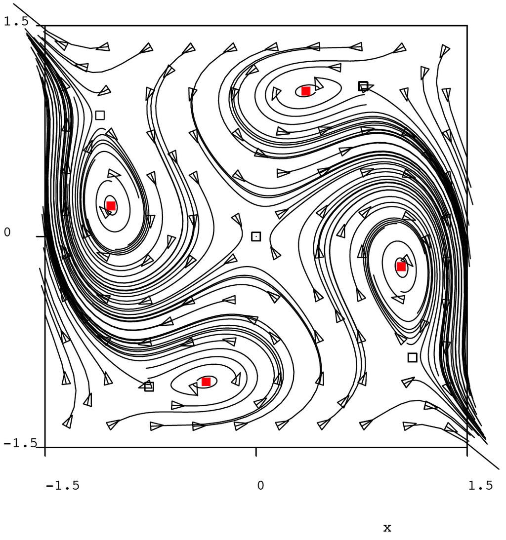
30 The following dia shows trajectories and steady states (stable: red squares, unstable: empty squares). The nature of the steady states is exactly as expected from the preliminary, qualitative, analysis (in particular, the orientations of the separatrices of the saddle points and the clockwise vs counter clockwise rotation of the trajectories around the foci)

31

32 4. From Jacobian matrix to eigenvalues and eigenvectors.

33 Eigenvalues Like any matrix, the jacobian matrix J can be characterized by its eigenvalues. Det(J " I#) = 0 is the «characteristic equation» of matrix J (I is the identity matrix) and the eigenvalues are the values of lambda for which that equation has non-trivial roots, this is, for which the determinant of the characteristic equation is nil.

34 Physical meaning of the eigenvalues In nonlinear systems, the eigenvalues are of course functions of the location in phase space. The signs of the eigenvalues tell whether a direction is attractive (-) or repulsive (+), and characterize thus the nature of the steady states.

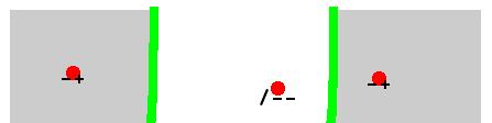
35 " + + means # $ % an unstable node & & ' ' means % $ # a stable node "

36 " # + means $ % & a saddle point '

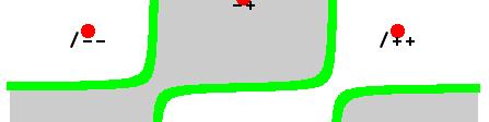
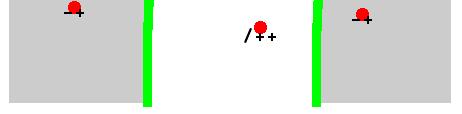
37 Complex eigenvalues " Periodic motion / + + " an unstable focus / # # " a stable focus

38 Eigenvectors Once the characteristic equation solved in lambda, the solutions in x, y, z are the eigenvectors of matrix J. Physical meaning of the eigenvectors: Orientation of the flow near steady states

39 5. FRONTIERS Phase space can be partitioned according to the signs of the eigenvalues (and if required, to the slopes of the eigenvectors). This provides a global view of the structure of phase space.

40 System B x = "x + x 3 " 0.2y 2 y = 0.3x 2 + y " y 3

41 Jacobian matrix of system B #"1+ 3x 2 "0.2y % $ +0.3x 1" 3y 2 & ( '

42 ( green ) Frontier F1 First step: partition according to the sign of the product (P) of the eigenvalues. As P = det[j], the equation of F1 is simply Det[J] = 0, and this, whatever the number of variables. In white, the positive regions (det[j] > 0 In gray, the negative regions (det[j] < 0

43

44 ( blue ) Frontier F2 In order to partition according to the signs of the eigenvalues (and not only to the sign of their product) one needs a second frontier. Frontier F2 is a variety (in 2D, a line) along which the real part of complex eigenvalues is nil. In 2D, F2 is defined by j 11 + j 22 = 0, with the constraint det[j] > 0

45

46 From now on each domain is homogeneous as regards the signs of the eigenvalues. This means that the signs of the eigenvalues of any steady state that would be present in a domain are determined by its very location in this domain.

47

48 ( dotted Boundary F4 (red, However, one still does not distinguish a pair of complex conjugate eigenvalues from a pair of real values of the same sign (/ + + from ++, or / - - from - -). Boundary F4 deals a domain according to the presence or absence of complex conjugate eigenvalues.

49 The equation of F4 is of course d = 0, in which d is the discriminant of the characteristic equation.

50

51 This diagram applies not only to system B proper, but as well to any system that differ from it only by non-zero terms in the ODE s. All these systems share the same Jacobian matrix, and thus the same frontiers, but the number and location of the steady states depend on the non-zero terms. For system B proper, the steady states are as follows:

52

53 It can be checked that the nature of the steady states is exactly as expected from the preliminary qualitative approach.

54 Note that there is no steady state in the complex crescents. Would it be possible to move a steady state to one of these regions? In fact, adding zero-order terms in the ODE's does not alter the Jacobian matrix, but changes the location of steady states, and in this way any point of phase space can be rendered steady.

55 In order to render any point, say {x 0, y 0 }, steady, it suffices to add proper zero-order terms to the ODE s: x = f x (x,y)" k, with k = f x (x 0,y 0 ) y = f y (x,y)" m, with m = f y (x 0,y 0 )

56 In the present case, to render point {0.15, 0.8} steady, one puts k = f x (0.15, 0.8) = m = f y (0.15, 0.8) =

57

58 In the present case, two steady states are present in one of the complex crescents. One of them is a stable focus, the other one, an unstable focus, as expected from their location.

59 When one adds a zero-order term to one of the ODE s, pairs of steady states converge, eventually collide and vanish, replaced by a pair of complex roots of the steady state equations (a bifurcation, as seen in phase space).

60

61 6. Auxiliary frontiers based on the slopes of the eigenvectors ( 2D (so far only in

62 For short, adjacent steady states of the same «species» (same signs of the eigenvalues) can usually be separated by additional, auxiliary frontiers based on the slopes of the eigenvectors.

63 In 2 dimensions ( 0 = (F2 : j 11 +j 22 F3: j 11 - j 22 =0 F5: j 12 +j 21 =0 F6: j 12 - j 21 =0 correspond to various relative slopes of the eigenvectors (opposite, inverse and normal, respectively).

64

65 The three saddle points on the diagonal are generated by different sign patterns of the (1+1)-nucleus, and consequently their separatrices display contrasting orientations. These steady states (and their regions) can be separated by an F3 frontier (j 11 - j 22 = 0).

66

67 Consider now system B: x = 0.2x 2 + y " y 3 y = x " x 3 " 0.2y 2 Whose Jacobian matrix is: # 0.4 x 1" 3y 2 & % $ 1" 3x 2 ( "0.4y '

68

69 In the preceding dia, one sees (frow N-W to S-E): - two stable foci that have to run one clockwise, the other counter clockwise - three saddle points with contrasting orientations - two unstable foci, one clockwise, the other counterclockwise. - All these steady states can be separated from each other by F5 (mauve) or F6 (turquoise) frontiers.

70

71 7. A single steady state per domain???

72 In most cases the frontiers partition phase space in such a way that all steady states are separated from each other, as if two adjacent steady states had to differ either by the signs of their eigenvalues or by the slopes of their eigenvectors (= as if each domain was a nest for a unique potential steady state).

73 In fact, I have a counter-example (two stable foci that are not separated by the partition process: Either the idea : not more than a single steady state per domain is incorrect Or there is still a frontier lacking

74 x = 0.6xy + y " y y = x " x xy Whose Jacobian matrix is: # 0.6y 0.6x +1" 3y 2 & % 1" 3x 2 ( $ + 0.4y 0.4x '

75

76 8.How many variables?

77 The major frontiers F1, F2 and F4 are in principle computable for n variables, although the process is heavier and heavier as n increases.

78 A diagram has to be visualised in 2 or at most 3-D. General case: a tomography using 2D sections of the nd phase space. BUT... if only 2 variables «carry» a nonlinearity, an n-dimensional system reduces to a 2-dimensional diagram.

79 Probably not useful for the top-down approach (I hope) very useful for the bottom-up approach.

80 RESERVE

81 Synthetic mode. A new type of deterministic chaos ( labyrinth chaos ).

82 Deterministic chaos can be described in a simple way as an extension of periodicity such that the trajectories never close up. More accurately, they are characterised by at least one positive Lyapunov exponent (an extension of the concept of eigenvalues). We have all reasons to believe that a necessary condition for a chaotic behaviour is the presence of at least a positive circuit (for multistationarity) and a negative circuit (for periodicity).

83 In nonlinear systems, terms of the Jacobian matrix, and thus circuits can be positive or negative depending to the location in phase space ( ambiguous circuits ). Is it then possible to generate deterministic chaos with a single circuit, provided it is ambiguous? Yes.

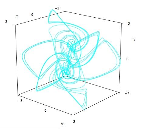
84 x = "bx + y " y 3 y = "by + z " z 3 z = "bz + x " x 3 Whose Jacobian matrix is: $ "b 1" 3y 2 # ' & # "b 1" 3z 2 ) & ) & % 1" 3x 2 ) # "b (

85 The sign of 1-3x 2 is + for small absolute values of x (more precisely, x < 1/ ), negative elsewhere, and similarly for y and z. Phase space is thus partitioned into 3 3 = 27 boxes according to the sign patterns of the 3-circuit. For sufficiently low values of the unique parameter b there are 3 3 = 27 steady states, all unstable.

86

87 The trajectories are chaotic (one or two chaotic attractors) with periodic windows (up to 6 limit cycles). So far we have not only a 3-circuit, but in addition three 1-circuits (the diagonal terms of the Jacobian matrix).

88 In fact, x-x 3 is a gross caricature of sin(x): the first two terms of the Taylor development are x-x 3 /3!) x = "bx + sin y y = "by + sinz z = "bz + sin x $ "b cos y # ' & ) # "b cosz & ) % cos x # "b (

89 In this system, as the unique parameter b decreases the number of steady states (all unstable) steadily increases, as well as the size and complexity of the attractors. The trajectories are chaotic (up to 6 chaotic ( cycles attractors) with periodic windows (up to 6 limit For b = 0 (now, a single circuit), there are an infinity of steady states that occupy the totality of phase space. There are no more attractors. Instead, the trajectories are chaotic (but not random) walks throughout phase space (labyrinth chaos)

90 Analogy with a big bang ( gros boum ( French in

91 RESERVE

92 I mentioned above that in system A the 2-nucleus is dominant almost everywhere in phase space. What does it mean? The weight of a nucleus can be measured as the absolute value of the product of the elements of the Jacobian matrix that constitute this nucleus. Along the line j 11 j 22 = j 12 j 21 the two nucleii of a 2-D system have the same weight, on one side of the line the2-nucleus dominates, on the other side, it is the (1+1)-nucleus.

93

94 Two bacterial cultures genetically identical and in identical condition may develop durably (>150 cell generations) different phenotypes if one of them has been submitted to a brief signal (brief presence of an inducer ): probably the most beautiful case of epigenetic differences... and multistationarity.