Cosc 3451 Signals and Systems. What is a system? Systems Terminology and Properties of Systems

Size: px

Start display at page:

Download "Cosc 3451 Signals and Systems. What is a system? Systems Terminology and Properties of Systems"

Jayson Blair
5 years ago
Views:

1 Cosc 3451 Signals and Systems Systems Terminology and Properties of Systems What is a system? an entity that manipulates one or more signals to yield new signals (often to accomplish a function) can be thought of as an interconnection of components, devices and subsystems (operations) Figure 1.2 (p. 3) Elements of a communication system. The transmitter changes the message signal into a form suitable for transmission over the channel. The receiver processes the channel output (i.e., the received signal) to produce an estimate of the message signal. 1

$The surface of the 70-meter reflector must remain accurate within a fraction of the signal s wavelength. (Courtesy of Jet Propulsion Laboratory.) Figure 1.4 (p.$

2 Figure 1.3 (p. 5) (a) Snapshot of Pathfinder exploring the surface of Mars. (b) The 70-meter (230- foot) diameter antenna located at Canberra, Australia. The surface of the 70-meter reflector must remain accurate within a fraction of the signal s wavelength. (Courtesy of Jet Propulsion Laboratory.) Figure 1.4 (p. 7) Block diagram of a feedback control system. The controller drives the plant, whose disturbed output drives the sensor(s). The resulting feedback signal is subtracted from the reference input to produce an error signal e(t), which, in turn, drives the controller. The feedback loop is thereby closed. x[n] x(t) Discrete-time System Continuous-time System y[n] y(t) Where H{} is a function describing the overall action of the system 2

3 Systems can be connected in: Series: In H 1 H 2 Out H 1 Parallel: In + H 2 Out Feedback: In + H 1 Out H 2 and various other combinations Figure 2.32 (p. 162) Symbols for elementary operations in block diagram descriptions of systems. (a) Scalar multiplication. (b) Addition. (c) Integration for continuous-time systems and time shifting for discrete-time systems. Figure 1.50 (p. 54) Discrete-time-shift operator S k, operating on the discrete-time signal x[n] to produce x[n k]. 3

Figure 1.51 (p. 54) Two different (but equivalent) implementations of the moving-average system: (a) cascade form of implementation and (b) parallel form of implementation.

4 Figure 1.51 (p. 54) Two different (but equivalent) implementations of the moving-average system: (a) cascade form of implementation and (b) parallel form of implementation. Properties Memory if system output y[n] {or y(t)} depend on previous values of system input x[n] or output y[n] it exhibits memory, i.e. if y[n] depends only on x[n] it is memoryless Causality in a causal system, outputs depend only on current and previous inputs, e.g. y[n] = x[n-2] (delay) if output of system depends on future values it is not causal, e.g. y[n] = x[n+2] (advance) physical systems/real-time systems are causal 4

5 Stability a stable system gives a bounded output, y[n], for a bounded input, x[n] Tacoma narrows bridge 5

6 Figure 1.69 (p. 79) Block diagram of first-order recursive discrete-time filter. The operator S shifts the output signal y[n] by one sampling interval, producing y[n 1]. The feedback coefficient p determines the stability of the filter. Time/shift invariance behaviour of a time-invariant (shift-invariant) system is fixed over time doesn t burn in, age, learn, adapt let y 1 [n] be the output of system to x 1 [n] then for shift invariance, the output y 2 [n] to input x 2 [n] = x 1 [n-n 0 ] must be y 2 [n] = y 1 [n-n 0 ] for all n 0 and x 1 [n] Figure 1.55 (p. 61) The notion of time invariance. (a) Time-shift operator S t0 preceding operator H. (b) Time-shift operator S t0 following operator H. These two situations are equivalent, provided that H is time invariant. 6

7 Figure 1.68 (p. 78) Tapped-delay-line model of a linear communication channel, assumed to be time-invariant. Linearity A linear system satisfies the principle of superposition, that is linearity is a very important and useful property never met in physical systems but useful approximation superposition property means that response to a complex input is the superposition of responses to components of the input, this will prove very useful if input is always zero, then output will always be zero. Useful in justifying the assumption of conditions of initial rest in LTI systems. 7

8 Figure 1.56 (p. 64) The linearity property of a system. (a) The combined operation of amplitude scaling and summation precedes the operator H for multiple inputs. (b) The operator H precedes amplitude scaling for each input; the resulting outputs are summed to produce the overall output y(t). If these two configurations produce the same output y(t), the operator H is linear. Figure 1.53 (p. 59) Series RC circuit driven from an ideal voltage source v 1 (t), producing output voltage v 2 (t). Figure 1.64 (p. 73) Mechanical lumped model of an accelerometer. 8

9 Figure 1.54 (p. 59) The notion of system invertibility. The second operator H inv is the inverse of the first operator H. Hence, the input x(t) is passed through the cascade correction of H and H -1 completely unchanged. LTI Systems a very important class of systems are the Linear Time-Invariant (LTI) systems linearity and sampling/sifting properties of the pulse/impulse give us the convolution sum and integral representations of response of systems sampling property superposition: signal can be represented as a combination of a number of component signals, i.e. shifted/delayed pulses or impulses in LTI system overall output is superposition of responses to the component signals 9

10 Sifting sum (discrete): Σ Sifting integral (continuous): integral is sum of impulse samples of x(t) placed infinitely close together (fig 2.12) Convolution Sum and Integral Discrete (Convolution Sum): input can be represented as a sum (sifting sum)of appropriately shifted and scaled pulses in LTI system, overall output is superposition of responses to these pulses if response to input is H{x[n]} then response to each pulse in the sifting sum is shifted and scaled version of h[n] = H{δ[n]} example (on board) 10

11 if system is time-invariant, h[n] is constant for impulse at any n x[n] H{} y[n] for each y[n] need to evaluate a set of signals, v k [n] = x[k]h[n-k] and sum over k OR consider h[n-k] = h[-(k-n)], reflected and timeshifted version (by n) of h[k] h[k] h[-k] evaluate one signal at each interval, w n [k]=x[k]h[n-k] and sum it up over k 11

Figure 2.1 (p. 99) Graphical example illustrating the representation of a signal x[n] as a weighted sum of time-shifted impulses. Figure 2.2a (p. 100) Illustration of the convolution sum.

12 Figure 2.1 (p. 99) Graphical example illustrating the representation of a signal x[n] as a weighted sum of time-shifted impulses. Figure 2.2a (p. 100) Illustration of the convolution sum. (a) LTI system with impulse response h[n] and input x[n]. commutativity: h[n]* x[n]= x[n]* h[n] distributivity: h[n]*(x[n] + z[n]) = h[n]* x[n] + h[n]* z[n] associativity: h[n]* (x[n]* z[n]) = ( h[n]* x[n] )* z[n] 12

Continuous (Convolution integral) directly analogous to discrete case each impulse in sifting integral drives an impulse response; like discrete case but infinitely close together manual method 1.

13 Continuous (Convolution integral) directly analogous to discrete case each impulse in sifting integral drives an impulse response; like discrete case but infinitely close together manual method 1. Graph x(τ), h(τ) as a function of τ. To get function h(t-τ) reflect h(τ) about τ=0 and time shift-t 2. begin with t large, negative 3. obtain functional form of x(τ) h(t-τ) = w t (τ). This is often constant for a range of t. 4. Integrate w t (τ) from τ = - to to get y[n] for each time t examples 13

14 Properties of LTI Systems and Convolution Parallel System x(t) h 1 (t) h 2 (t) y 1 (t) + y 2 (t) y(t) x[n] h 1 [n] h 2 [n] y 1 [n] + y 2 [n] y[n] Series System x[n] y[n] h 1 [n] h 2 [n] h 12 [n] 14

Figure 2.21 (p. 131) (a) Reduction of parallel combination of LTI systems in upper branch of Fig. 2.20.

2.21(b) to obtain an equivalent system for Fig. 2.20.

15 Figure 2.21 (p. 131) (a) Reduction of parallel combination of LTI systems in upper branch of Fig (b) Reduction of cascade of systems in upper branch of Fig. 2.21(a). (c) Reduction of parallel combination of systems in Fig. 2.21(b) to obtain an equivalent system for Fig Memoryless but memoryless system can only depend on x[n] and cannot depend on x[n-k] for k 0 Causality causal system cannot respond to input before it occurs y[n] cannot depend on x[n-k] for (n-k) > n, i.e. for k <0 15

16 BIBO Stability Step response 16

Response to sinusoid/complex exponential (preview of Fourier Transform) H(jω) is a function of ω not t -> frequency response in general it is complex amplitude response

17 Response to sinusoid/complex exponential (preview of Fourier Transform) H(jω) is a function of ω not t -> frequency response in general it is complex amplitude response phase response input is sinusoid/periodic exponential of frequency, ω. Output is same frequency sinusoid with magnitude H(jω) *A x and phase equal to input phase + arg(h(jω)) 17

18 Bode plot for discrete, we only need to plot from -π to π Where do h[n], h(t) come from? until now we ve assumed they are known LTI systems can be described by linear constant coefficient difference/differential equations h(t) or h[n] is the solution of these LCCDEs to a impulse/pulse forcing function solving LCCDE with appropriate initial conditions and impulse/pulse input give h(t)/h[n] 18

homogeneous solution to differential equation on its own is not sufficient; we need to define auxiliary

19 Continuous-time impulse response recall: N-th order LCCDE to solve for y(t) need two sub-solutions: the forced response: a particular solution which depends on the input x(t) the natural response: a homogeneous solution to differential equation on its own is not sufficient; we need to define auxiliary (initial) conditions to determine the response Usually assume initial rest, that is is x(t) = 0 for t <= t 0 then 19

20 causal LTI systems imply this condition no stored energy/memory when no input has been applied Thus, causal LTI systems (an important class of real world systems) can be described by a LCCDE under conditions of initial rest for an LTI system the forced response (particular solution) is linear with respect to the input also, natural response is linear with respect to the initial conditions but complete response is not therefore, for time invariance we need conditions of initial rest so that output does not depend on timing of input except for a time shift so for h(t), we need to solve LCCDE for impulse input (note that impulse response is a function of the terms in natural response) see 2.56 for one way another way is to find s(t), the step response or the solution of the LCCDE with u(t) as input use transform techniques 20

21 Discrete-time pulse response N-th order Linear Constant Coefficeint Difference Equations need to know y[-1].. y[-n] as initial conditions to calculate y[0] if x[n] = 0 for n<n 0 then conditions of initial rest are y[n 0 -N] = y[n 0 -N+1]= = y[n 0-1]=0 LCCDE with conditions of initial rest give casual LTI systems IIR system y[n] depends on previous values of y recursively impulse response can be infinite in length (infinite impulse response or IIR) since effects of input values before x[n-m] are stored FIR system if N = 0 y[n] can only be influenced by the previous M values of x finite impulse response (FIR) 21

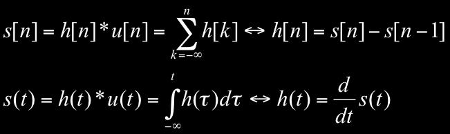
Solution of h[n] (a function of terms in natural response): find s[n], h[n] = s[n]-s[n-1] algebraically rearrange for y[n] in terms of x[n], x[n-1], and y[n], y[n-1], and solve for x[n] = δ[n] and

22 Solution of h[n] (a function of terms in natural response): find s[n], h[n] = s[n]-s[n-1] algebraically rearrange for y[n] in terms of x[n], x[n-1], and y[n], y[n-1], and solve for x[n] = δ[n] and initial rest conditions, e.g. closed form solution (e.g. problem 2.55) for FIR (or truncated IIR) apply δ[n] and solve for h[n] only over the M intervals use transform methods Figure 2.37 (p. 166) Block diagram representations of a continuous-time LTI system described by a second-order integral equation. (a) Direct form I. (b) Direct form II. 22

Analog vs. discrete signals

Analog vs. discrete signals Continuous-time signals are also known as analog signals because their amplitude is analogous (i.e., proportional) to the physical quantity they represent. Discrete-time signals