Binomial Logis5c Regression with glm()

Transcription

1 Friday 10/10/2014

2 Binomial Logis5c Regression with glm()

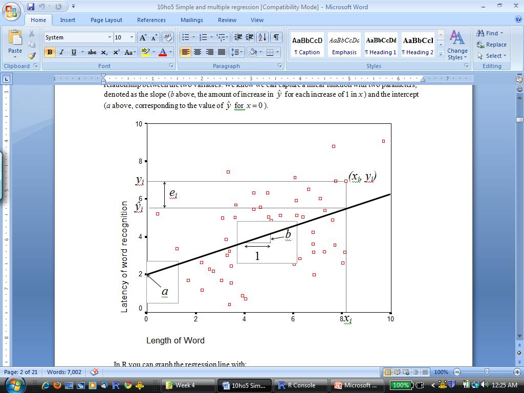
3 > plot(x,y) > abline(reg=lm(y~x))

4 Binomial Logis5c Regression numsessions relapse No relapse 1.15 No relapse 1.87 No relapse.62 No relapse -.47 Relapse.88 No relapse -.99 Relapse.81 No relapse.44 No relapse Relapse.52 No relapse.14 Relapse -.49 Relapse.60 No relapse -.03 No relapse -.43 Relapse -.94 Relapse -.06 Relapse -.84 Relapse Relapse

5

6 The Logis5c Func5on 1 e x 1+ e x 0 x

7 The Exponen5al Func5on e x e = log(e x ) = x e log(x) = x e x * e Y = e x+y e 0 = 1 > curve(exp(x),-5,+5) > rbind(-3:3,round(exp(-3:3),2)) [,1] [,2] [,3] [,4] [,5] [,6] [,7] [1,] [2,]

8 y p p e p p p e p e p e p e pe p e e p e e p y y y y y y y y y y ˆ 1 log 1 ) (1 * ) (1 1 ˆ ˆ ˆ ˆ ˆ ˆ ˆ ˆ ˆ ˆ = = = = = + = + + = x x e e 1+ logit = log(p/(1- p)) The Logis5c Func5on 0 1 x

9 > glm(relapse~numsessions,family="binomial") Call: glm(formula = relapse ~ numsessions, family = "binomial") Coefficients: (Intercept) numsessions Degrees of Freedom: 19 Total (i.e. Null); 18 Residual Null Deviance: Residual Deviance: AIC: p( relapse) log 1 ( ) p relapse = * Numsessions.186 At numsess = 0 (i.e. at the mean) p( relapse) log 1 p( relapse) =.186 p relapse) 1 p( relapse) (. 186 = e =.83 At numsess = 1 p relapse) 1 p( relapse) ( = e =.10 At numsess = - 1 p relapse) 1 p( relapse) ( = e = 6.73

10 e 1+ e yˆ e p = 1+ e * Numsessions p ( relapse) = * Numsessions yˆ At mean numssessions (0) p(relapse) = 45% At high numssessions (+1) p(relapse) = 9% At low numssessions (- 1) p(relapse) = 87% a< ; b< numsessions<-seq(-3,3,by=.01) p_relapse<-exp(a+b*numsessions)/(1+exp(a+b*numsessions)) plot(numsessions,p_relapse,cex=.5,col="blue")

11 b = - 20 b = - 5 b = - 1 b = +5

12 Mul5ple Regression

13 Mul5ple Regression y ˆ = a + bx ˆ = b b x b x b x y yˆ = bi xi + b 0

14 ID GPA SAT GPA Reco (College) (%) (High) id coll_gpa sat recs hs_gpa > round(cor(data0),2) ID coll_gpa sat recs hs_gpa ID coll_gpa sat recs hs_gpa

15 > summary(lm(coll_gpa~sat,data=data0)) Coefficients: Estimate Std. Error t value Pr(> t ) (Intercept) ** sat *** --- Residual standard error: on 18 degrees of freedom Multiple R-squared: , Adjusted R-squared: F-statistic: on 1 and 18 DF, p-value: > summary(lm(coll_gpa~sat+recs,data=data0)) Coefficients: Estimate Std. Error t value Pr(> t ) (Intercept) ** sat *** recs * --- Residual standard error: on 17 degrees of freedom Multiple R-squared: , Adjusted R-squared: F-statistic: 15.5 on 2 and 17 DF, p-value: > summary(lm(coll_gpa~sat+hs_gpa,data=data0)) Coefficients: Estimate Std. Error t value Pr(> t ) (Intercept) ** sat * hs_gpa * --- Residual standard error: on 17 degrees of freedom Multiple R-squared: , Adjusted R-squared: F-statistic: on 2 and 17 DF, p-value:

16 sat hs_gpa model2$residuals hs_gpa coll_gpa model2$residuals (SAT controlling for hs_gpa)

17 > round(cor(hs_gpa,model2$residuals),3) [1] 0 > summary(lm(coll_gpa~model2$resid)) Coefficients: Estimate Std. Error t value Pr(> t ) (Intercept) <2e-16 *** model2$resid Residual standard error: on 18 degrees of freedom Multiple R-squared: ,Adjusted R-squared: F-statistic: on 1 and 18 DF, p-value: Standardized Coefficients b s β i i i = s 0 Residual Variance MS Re sidual ( Y = MSError = N Yˆ) p 1 2 See lm.beta() in package QuantPsyc Note that this is the square of the residual standard error above or the standard error of the esmmate (s Y.X )

18 > summary(lm(coll_gpa~hs_gpa+sat+recs,data=data0)) Call: lm(formula = coll_gpa ~ hs_gpa + sat + recs, data = data0) Residuals: Min 1Q Median 3Q Max Coefficients: Estimate Std. Error t value Pr(> t ) (Intercept) ** hs_gpa sat * recs * --- Signif. codes: 0 *** ** 0.01 * Residual standard error: on 16 degrees of freedom Multiple R-squared: , Adjusted R-squared: F-statistic: on 3 and 16 DF, p-value: > confint(lm(coll_gpa~sat+hs_gpa,data=data0)) 2.5 % 97.5 % (Intercept) hs_gpa sat recs

19 R = r YY ˆ This is the mulmple correlamon coefficient. > cor(coll_gpa,lm(coll_gpa~sat+hs_gpa)$fitted) [1] > cor(coll_gpa,lm(coll_gpa~sat+hs_gpa)$fitted)^2 [1] > summary(lm(coll_gpa~sat+hs_gpa,data=data0)) Coefficients: Estimate Std. Error t value Pr(> t ) (Intercept) ** sat * hs_gpa * --- Residual standard error: on 17 degrees of freedom Multiple R-squared: , Adjusted R-squared: F-statistic: on 2 and 17 DF, p-value:

20 r YY R ˆ = 1 1) )( ( = p N N R adjr ) (1 1) ( 2 2 R p R p N F =, with (p, N-p-1) degrees of freedom. ) )(1 ( ) 1)( ( 1) /( ) ) /( ( ), ( f r f f r f f N r f R r f R R f N f N SSE r f SSR SSR F = =

21 F ( f r, N f 1) = ( SSR f SSE f SSR r ) /( f /( N f 1) r) = ( N ( f f 1)( R 2 f r)(1 R 2 f R ) 2 r ) > length(coef(model2))-1->f > length(coef(model3))-1->r > length(data0$coll_gpa)->n > summary(model2)[8][[1]]->r2f > summary(model3)[8][[1]]->r2r > > (N-f-1)*(R2f-R2r)/((f-r)*(1-R2f)) [1] > anova(model2,model3) Analysis of Variance Table Model 1: coll_gpa ~ hs_gpa + sat + recs Model 2: coll_gpa ~ sat + recs Res.Df RSS Df Sum of Sq F Pr(>F) Signif. codes: 0 *** ** 0.01 *

22 Par5al Correla5on > round(cor(data1),2) r y1 2 = r y1 (1 r r r y2 )(1 r 2 y2 ) icecream drownings heat icecream drownings heat > bm.partial<-function(x,y,z) {round((cor(x,y)-cor(x,z)*cor(y,z))/sqrt((1- cor(x,z)^2)*(1-cor(y,z)^2)),2)} > ls() [1] "bm.partial" "data1" > bm.partial(data1$icecream,data1$drownings,data1$heat) [1] 0.08 # Now I am repeating it with the formula from the psych package > library(psych) > partial.r(data1,1:2,3) icecream drownings icecream drownings # Note that we obtain the same result by correlating residuals: > cor(lm(icecream~heat,data=data1)$residuals,lm(drownings~heat,data=data1)$residuals) [1]

23 Semi- Par5al (Part) Correla5on r 0(1 2) = ( r 01 r 02 (1 r r ) ) > round(cor(data2),2) racetime practicetime practicetrack racetime practicetime practicetrack > bm.semipartial<-function(x,y,z) {round((cor(x,y)-cor(x,z)*cor(y,z))/sqrt((1- cor(y,z)^2)),2)} > bm.semipartial(racetime,practicetime,practicetrack) [1] 0.39 # Note that you get a very similar result by correlating a residual with racetime # But in contrast to the partial correl, only one of the two terms is a residual here. > cor(data2$racetime,lm(practicetime~practicetrack,data=data2)$residuals) [1]

24 Breaking Down the SS X 0 a e b c f d g X 1 X 2

25 R 2 can be high while none of the predictors are significant! > summary(lm(y2~x3+x4,data=data3)) Coefficients: Estimate Std. Error t value Pr(> t ) (Intercept) X X Residual standard error: 2.31 on 24 degrees of freedom Multiple R-squared: , Adjusted R-squared: F-statistic: on 2 and 24 DF, p-value: 5.68e-09 > cor(data3[,7:9]) X3 X4 Y2 X X Y Y 2 a b c X 3 d X 4

26 > summary(lm(y~x1,data=data3)) Coefficients: Estimate Std. Error t value Pr(> t ) (Intercept) X * --- Residual standard error: on 25 degrees of freedom Multiple R-squared: , Adjusted R-squared: F-statistic: on 1 and 25 DF, p-value: > summary(lm(y~x2,data=data3)) Coefficients: Estimate Std. Error t value Pr(> t ) (Intercept) X ** --- Residual standard error: on 25 degrees of freedom Multiple R-squared: , Adjusted R-squared: F-statistic: on 1 and 25 DF, p-value: > summary(lm(y~x1+x2,data=data3)) Coefficients: NoMce how the coefficient for X2 goes up even as it gets less significant. Estimate Std. Error t value Pr(> t ) (Intercept) X X * --- Residual standard error: on 24 degrees of freedom Multiple R-squared: , Adjusted R-squared: F-statistic: on 2 and 24 DF, p-value:

27 X X2.1 (Residuals) X X1

28 > lm(x1~x2,data=data3)$residuals->data3$x1.2 X1 X2 Y X2.1 X1.2 X X Y X X

29 > summary(lm(y~x1.2,data=data3)) Coefficients: Estimate Std. Error t value Pr(> t ) (Intercept) ** X Residual standard error: on 25 degrees of freedom Multiple R-squared: 2.438e-05, Adjusted R-squared: F-statistic: on 1 and 25 DF, p-value: > summary(lm(y~x2.1,data=data3)) Coefficients: Estimate Std. Error t value Pr(> t ) (Intercept) *** X Residual standard error: on 25 degrees of freedom Multiple R-squared: , Adjusted R-squared: F-statistic: on 1 and 25 DF, p-value: > summary(lm(y~x1+x2.1,data=data3)) Coefficients: Estimate Std. Error t value Pr(> t ) (Intercept) X * X * --- Residual standard error: on 24 degrees of freedom Multiple R-squared: , Adjusted R-squared: F-statistic: on 2 and 24 DF, p-value:

30 > summary(lm(y~x1.2+x2.1,data=data3)) Coefficients: Estimate Std. Error t value Pr(> t ) (Intercept) *** X * X ** --- Residual standard error: on 24 degrees of freedom Multiple R-squared: , Adjusted R-squared: F-statistic: on 2 and 24 DF, p-value: Y 68% X 2 14% 18% X 1 Predictors: X1 X1.2 X2 X2.1 Intercept R 2 X1 14.5* X2 1.2** X1 and X * X **.00 X **.14 X1 and X * 1.2* X2 and X ** X1.2 and X * 2.7** 45.3**.32

31 Monday 10/13/2014

32 > names(model1) [1] "coefficients" "residuals" "effects" "rank" "fitted.values" [6] "assign" "qr" "df.residual" "xlevels" "call" [11] "terms" "model" > model1$fitted > model1$residuals > model1$df [1] 18

33 WARNING: anova(lm()) parmmons the sum of square sequenmally so order of predictor maaers! > summary(lm(y~x1)) (Intercept) *** x * > summary(lm(y~x2)) (Intercept) e-11 *** x > summary(lm(y~x1+x2)) (Intercept) *** x x > summary(lm(y~x2+x1)) (Intercept) *** x x Signif. codes: 0 *** ** 0.01 * Residual standard error: on 97 degrees of freedom Multiple R-squared: , Adjusted R-squared: F-statistic: on 2 and 97 DF, p-value: In lm() the order does not maaer

34 > summary(lm(y~x2+x1)) (Intercept) *** x x Signif. codes: 0 *** ** 0.01 * Residual standard error: on 97 degrees of freedom Multiple R-squared: , Adjusted R-squared: F-statistic: on 2 and 97 DF, p-value: > anova(lm(y~x1+x2)) Df Sum Sq Mean Sq F value Pr(>F) x * x Residuals Now the order maaers! > anova(lm(y~x2+x1)) Df Sum Sq Mean Sq F value Pr(>F) x x Residuals

35 10 predict() > model1$call lm(formula = coll_gpa ~ hs_gpa) > predict(model1,list(hs_gpa=3.4)) Y X > model2$call lm(formula = coll_gpa ~ hs_gpa + sat + recs, data = data0) > predict(model2,list(hs_gpa=c(3.4,2.9),sat=c(60,90),recs=c(4,5))) > predict(model2,list(hs_gpa=c(3.4,2.9),sat=c(60,90),recs=c(4,5)), interval="confidence") fit lwr upr > predict(model2,list(hs_gpa=c(3.4,2.9),sat=c(60,90),recs=c(4,5)) interval="prediction") fit lwr upr For a discussion of predicmon vs. confidence intervals see: hap://en.wikipedia.org/wiki/predicmon_interval

36 > with(data0,plot(coll_gpa,hs_gpa)) > abline(model1) abline()

37 hap://cran.r- project.org/web/packages/scaaerplot3d/index.html (The easiest thing to do is to install it within R, or download the.zip here.) scaaerplot3d() with(data0,scatterplot3d(sat,recs,coll_gpa))

38 scaaerplot3d() with(data0,scatterplot3d(sat,recs,coll_gpa,pch=16,color="red"))

39 scaaerplot3d() with(data0,scatterplot3d(sat,recs,coll_gpa,pch=16,color="red",type="h"))

40 scaaerplot3d()$plane3d() > model3$call lm(formula = coll_gpa ~ sat + recs, data = data0) > with(data0,scatterplot3d(sat,recs,coll_gpa,pch=16,color="red",type="h"))->my3d > names(my3d) [1] "xyz.convert" "points3d" "plane3d" "box3d" > my3d$plane3d(model3)

41 Dummy Coding

42 Imagine a study with 50 par5cipants split unevenly into 3 groups (X) and measured on a dv Y. > str(d) 'data.frame': 50 obs. of 2 variables: $ x: num $ y: num > summary(d) x y Min. :1.00 Min. : st Qu.:1.00 1st Qu.: Median :2.00 Median : Mean :2.16 Mean : rd Qu.:3.00 3rd Qu.: Max. :3.00 Max. : > table(d$x) > round(tapply(d$y,d$x,mean),2)

43 In this first pass we treat X as if it was a con5nuous variable. > summary(lm(y~x,data=d)) Call: lm(formula = y ~ x, data = d) Coefficients: Estimate Std. Error t value Pr(> t ) (Intercept) e-08 *** x * --- Signif. codes: 0 *** ** 0.01 * Residual standard error: on 48 degrees of freedom Multiple R-squared: , Adjusted R-squared: F-statistic: on 1 and 48 DF, p-value:

44 > as.factor(d$x)->d$x > summary(lm(y~x,data=d)) Call: lm(formula = y ~ x, data = d) Residuals: Min 1Q Median 3Q Max y ˆ = b + b x2 + b x Where x2 and x3 each take the values 0 or 1. Coefficients: Estimate Std. Error t value Pr(> t ) (Intercept) e-14 *** x * x * --- Signif. codes: 0 *** ** 0.01 * Residual standard error: 1.99 on 47 degrees of freedom Multiple R-squared: , Adjusted R-squared: F-statistic: on 2 and 47 DF, p-value: > tapply(d$y,d$x,mean)->means > means[2]-means[1] > means[3]-means[1] Now when X is a factor, lm() gives two dummy codes corresponding to the difference in means from Group 1.

45 > factor(sample(c("control","before","after"),50,replace=t))->d$z > str(d) 'data.frame': 50 obs. of 3 variables: $ x: Factor w/ 3 levels 1", 2", 3": $ y: num $ z: Factor w/ 3 levels "After","Before",..: > summary(lm(y~z,data=d)) Call: lm(formula = y ~ z, data = d) Residuals: Min 1Q Median 3Q Max As is illustrated here, the reference group is the one earliest in the alphabet*, which can be arbitrary [* on values, not labels; here Level 1 is Ader ] Coefficients: Estimate Std. Error t value Pr(> t ) (Intercept) <2e-16 *** zbefore zcontrol Signif. codes: 0 *** ** 0.01 * Residual standard error: on 47 degrees of freedom Multiple R-squared: , Adjusted R-squared: F-statistic: on 2 and 47 DF, p-value:

46 > contrasts(d$x) > d[d$x==1,4]<-0 > d[d$x==2,4]<-1 > d[d$x==3,4]<-0 > d[d$x==1,5]<-0 > d[d$x==2,5]<-0 > d[d$x==3,5]<-1 y ˆ = b + b1 x2 + b2 0 x Where x2 and x3 each take the values 0 or 1. > str(d) 'data.frame': 50 obs. of 5 variables: $ x : Factor w/ 3 levels "1","2","3": $ y : num $ z : Factor w/ 3 levels "After","Before",.. $ myx2: num $ myx3: num I want to show you that the contrasts used by R is the same thing as you entered your own dummy coding. 3 > d x y z myx2 myx Control Control After Control Before Before After Control Before After After After Before After Before After Control After After After Before After After Before After Control Before After 0 1 ( )

47 > summary(lm(y~myx2+myx3,data=d)) Coefficients: Estimate Std. Error t value Pr(> t ) (Intercept) e-14 *** myx * myx * --- Signif. codes: 0 *** ** 0.01 * Residual standard error: 1.99 on 47 degrees of freedom Multiple R-squared: , Adjusted R-squared: F-statistic: on 2 and 47 DF, p-value: > summary(lm(y~x,data=d)) Coefficients: Estimate Std. Error t value Pr(> t ) (Intercept) e-14 *** x * x * --- Signif. codes: 0 *** ** 0.01 * These two numerical dummy codes give the same result as X as a factor. Residual standard error: 1.99 on 47 degrees of freedom Multiple R-squared: , Adjusted R-squared: F-statistic: on 2 and 47 DF, p-value: y ˆ = b0 + b1 x2 + b2 x Where x2 and x3 each take the values 0 or 1. 3

48 > summary(lm(y~x-1,data=d)) Call: lm(formula = y ~ x - 1, data = d) Coefficients: Estimate Std. Error t value Pr(> t ) x e-14 *** x e-15 *** x < 2e-16 *** --- Signif. codes: 0 *** ** 0.01 * Residual standard error: 1.99 on 47 degrees of freedom Multiple R-squared: 0.918, Adjusted R-squared: F-statistic: on 3 and 47 DF, p-value: < 2.2e-16 > means > 1.99/sqrt(tapply(d$y,d$x,length)) R lets you remove the intercept all 3 means are now tested against zero, using the residual s.e..

49 > summary(lm(y~1,data=d)) On the other hand, the model with only 1 has only an intercept in other words the grand mean. Coefficients: Estimate Std. Error t value Pr(> t ) (Intercept) <2e-16 *** Residual standard error: on 49 degrees of freedom > mean(d$y) [1] > sd(d$y) [1] > sd(d$y)/sqrt(49) [1] > sd(d$y)/sqrt(50) [1]

50 R uses the contrasts() command to specify how categorical variables should be handled. TradiMonally this transformamon of categorical variables with k values (k>2) into k- 1 numerical variables is called dummy coding, of which there are 3 major types: 1 Dummy coding 2 Effect coding 3 Contrast coding

51 > c('a1','a2','a3')->a > c('b1','b2','b3')->b Let me first remind you quickly how we can make a matrix from vectors using rbind() or cbind(). > rbind(a,b) #Bind as rows [,1] [,2] [,3] A "A1" "A2" "A3" B "B1" "B2" "B3 > cbind(a,b) #Bind as columns A B [1,] "A1" "B1" [2,] "A2" "B2" [3,] "A3" "B3"

52 > #Dummy coding (default) > contrasts(d$x) Dummy coding can be simply adjusted by inpu5ng a new matrix of codes into contrast(). Here this is the default matrix. > summary(lm(y~x,data=d)) Coefficients: Estimate Std. Error t value Pr(> t ) (Intercept) e-14 *** x * x * Residual standard error: 1.99 on 47 degrees of freedom Multiple R-squared: , Adjusted R-squared: F-statistic: on 2 and 47 DF, p-value: > means[2]-means[1] > means[3]-means[1]

53 > #Dummy coding (default) > contrasts(d$x)<-cbind(c(1,0,0),c(0,0,1)) > contrasts(d$x) [,1] [,2] Even if you s5ck to simple dummy coding, you can change which group is the reference group > summary(lm(y~x,data=d)) Coefficients: Estimate Std. Error t value Pr(> t ) (Intercept) e-15 *** x * x Residual standard error: 1.99 on 47 degrees of freedom Multiple R-squared: , Adjusted R-squared: F-statistic: on 2 and 47 DF, p-value: > means[1]-means[2] > means[3]-means[2]

54 > cbind(c(1,0,0),c(0,1,0),c(0,0,1))->c > contrasts(d$x)<-c > contrasts(d$x) [,1] [,2] No5ce what happens when you try to put more than (k- 1) dummy codes.

55 > #Dummy coding (default) > contrasts(d$x) > #Effect coding > contrasts(d$x)<-cbind(c(-1,1,0),c(-1,0,1)) > contrasts(d$x) [,1] [,2]

56 > #Effect coding > contrasts(d$x)<-cbind(c(-1,1,0),c(-1,0,1)) > summary(lm(y~x,data=d)) Coefficients: Estimate Std. Error t value Pr(> t ) (Intercept) <2e-16 *** x x Signif. codes: 0 *** ** 0.01 * Residual standard error: 1.99 on 47 degrees of freedom Multiple R-squared: , Adjusted R-squared: F-statistic: on 2 and 47 DF, p-value: > mean(d$y) [1] > mean(means) [1] > means[2]-mean(means) > means[3]-mean(means) Effect coding tests departures from the unweighted grand mean.

57 Contrast coding is best to capture Planned contrasts, a priori predic5ons you have made about the pamern of your means

58 Rules for contrast weights Contrast Contrast = a = a x 1 x a a x 2 x = +... = a 1. i a x 2. i i x i 1 Weights sum to zero 2 Orthogonal contrasts k i= 1 k i= 1 a j. i = 0 a1. ia2. i= 0 3 With k groups there are (k 1) orthogonal contrasts

59 > #Dummy coding (default) > contrasts(d$x) > #Effect coding > contrasts(d$x)<-cbind(c(-1,1,0),c(-1,0,1)) > contrasts(d$x) [,1] [,2] > #Contrast coding > contrasts(d$x)<-cbind(c(-2,1,1),c(0,-1,1)) > contrasts(d$x) [,1] [,2]

60 > #Contrast coding > contrasts(d$x)<-cbind(c(-2,1,1),c(0,-1,1)) > summary(lm(y~x,data=d)) Coefficients: Estimate Std. Error t value Pr(> t ) (Intercept) <2e-16 *** x ** x Signif. codes: 0 *** ** 0.01 * Residual standard error: 1.99 on 47 degrees of freedom Multiple R-squared: , Adjusted R-squared: F-statistic: on 2 and 47 DF, p-value: > mean(means) [1] > (-2)^2+(+1)^2+(+1)^2 [1] 6 > (-2*means[1]+means[2]+means[3])/ > (-means[2]+means[3])/ Contrast coding tests more surgical a priori predic5ons.

61 Contrast coding tests more surgical a priori predic5ons, and can be more complicated: Control Threat 1 Threat 2 Self- Affirma5on