The Laplace Transform

Size: px

Start display at page:

Download "The Laplace Transform"

Leo Franklin
5 years ago
Views:

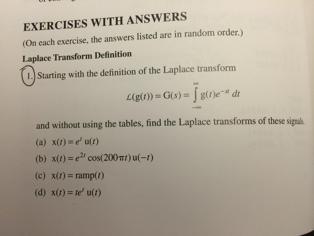
1 The Laplace Transform

2 Syllabus ECE 316, Spring 2015

3 Final Grades Homework (6 problems per week): 25% Exams (midterm and final): 50% (25:25) Random Quiz: 25%

4 Textbook M. Roberts, Signals and Systems, 2nd edition, McGraw- Hill, 2011 Chapter 8-16

5 Other information Course website: htm Office hour: 11am-12am MWF. TA: Ramin Nabati

6 Main Topics Basic Tools: Laplace Transform (continuous time system) Z Transform (discrete time system) Sampling (converting from continuous time system to discrete time system) Applications Filter Design Frequency Analysis State space

7 What You Can Do After This Course? Signal Aspect: Given a signal, you can analyze the spectrum and understand the characteristic (low pitch? high pitch?) You can sample the signal to obtain digitized signals. System Aspect: Given an input-output specification (say, filter out an interference in audio signal), you can design a simple filter (leave the detailed design to more advanced courses). Given a system, you can determine the stability and predict the output as a function of input frequency.

8 Foundation of Different Areas If you do not understand signals and systems, the following areas are forbidden: Communications Signal processing Audio/Image/Video processing Control Filter Design A-D Circuits et al

9 Keywords to be remembered after 10 years Laplace transform, poles, zeros, complex plane Z-transform, unit circle Sampling, Nyquist criterion, aliasing Low/high/band pass filter, Butterworth filter Frequency response, bandwidth Stability, system state Check this list when you complete the course.

10 Generalizing the Fourier Transform! The CTFT expresses a time-domain signal as a linear combination of complex sinusoids of the form e jωt. In the generalization of the CTFT to the Laplace transform, the complex sinusoids become complex exponentials of the form e st where s can have any complex value. Replacing the complex sinusoids with complex exponentials leads to this definition of the Laplace transform. L( x( t) ) = X s ( ) L x t ( ) = x t X s ( )e st dt ( ) 1/13/11! M. J. Roberts - All Rights Reserved! 2!

11 Generalizing the Fourier Transform! The variable s is viewed as a generalization of the variable ω of the form s = σ + jω. Then, when σ, the real part of s, is zero, the Laplace transform reduces to the CTFT. Using s = σ + jω the Laplace transform is ( ) = x t X s ( )e ( σ + jω )t dt = F x( t)e σt which is the Fourier transform of x( t)e σt 1/13/11! M. J. Roberts - All Rights Reserved! 3!

12 Generalizing the Fourier Transform! The extra factor e σt is sometimes called a convergence factor because, when chosen properly, it makes the integral converge for some signals for which it would not otherwise converge. For example, strictly speaking, the signal Au t ( ) does not have a CTFT because the integral does not converge. But if it is multiplied by the convergence factor, and the real part of s is chosen appropriately, the CTFT integral will converge. Au( t)e jωt dt Ae σt u( t)e jωt dt 0 = A e jωt dt Does not converge = A e ( σ + jω )t dt Converges (if σ > 0) 0 1/13/11! M. J. Roberts - All Rights Reserved! 4!

13 Complex Exponential Excitation! If a continuous-time LTI system is excited by a complex exponential x t ( ) = Ae st, where A and s can each be any complex number, the system response is also a complex exponential of the same functional form except multiplied by a complex constant. The response is the convolution of the excitation with the impulse response and that is ( ) = h τ y t ( )x( t τ )dτ = h τ The quantity H s of h( t). ( ) = h τ ( ) Ae s t τ ( ) dτ = Ae st h( τ )e sτ dτ 1/13/11! M. J. Roberts - All Rights Reserved! 5! x( t) ( )e sτ dτ is called the Laplace transform

14 Complex Exponential Excitation! Let x t ( ) = ( 6 + j3) e 3 j 2 A ( s ) t = ( )e ( 3 j 2)t and let h( t) = e 4t u( t). Then H( s) = 1, σ > 4 and, s + 4 in this case, s = 3 j2 = σ + jω with σ = 3 > 4 and ω = 2. y( t) = x( t)h( s) = 6 + j3 3 j2 + 4 e ( 3 j 2)t = ( )e ( 3 j 2)t. The response is the same functional form as the excitation but multiplied by a different complex constant. This only happens when the excitation is a complex exponential and that is what makes complex exponentials unique. 1/13/11! M. J. Roberts - All Rights Reserved! 6!

Pierre-Simon Laplace! 3/23/1749-3/2/1827!

16 The Transfer Function! Let x( t) be the excitation and let y( t) be the response of a system with impulse response h( t). The Laplace transform of y( t) is Y s ( ) = y t Y s ( )e st dt = h( t) x t ( ) = h τ Y s ( ) = h τ ( ) ( )x( t τ )dτ e st dt ( )dτ x( t τ )e st dt e st dt 1/13/11! M. J. Roberts - All Rights Reserved! 8!

17 The Transfer Function! Y s ( ) = h τ ( )dτ Let λ = t τ dλ = dt. Then Y s ( ) = h τ x( t τ )e st dt ( )dτ x( s( λ+τ ) λ)e dλ = h( τ )e sτ dτ x( λ)e sλ dλ H( s) X( s) Y( s) = H( s)x( s) H( s) is called the transfer function. y( t) = x( t) h( t) L Y( s) = H( s)x( s) 1/13/11! M. J. Roberts - All Rights Reserved! 9!

18 The Transfer Function! Let x( t) = u( t) and let h( t) = e 4t u( t). Find y( t). y( t) = x( t) h( t) = x τ y( t) = y t ( )h( t τ )dτ = u τ ( 4 t τ )e ( ) u ( t τ )dτ t t 4( t τ ) e 4t 1 1 e dτ = e 4t e 4τ dτ = e 4t e 4t =, t > , t < 0 ( )( 1 e 4t )u( t) ( ) = 1/ 4 X( s) = 1/ s, H( s) = 1 s + 4 Y ( s ) = 1 s 1 s + 4 = 1/ 4 s x( t) = ( 1/ 4) 1 e 4t ( ) ( )u t 1/ 4 s + 4 1/13/11! M. J. Roberts - All Rights Reserved! 10!

19 Cascade-Connected Systems! If two systems are cascade connected the transfer function of the overall system is the product of the transfer functions of the two individual systems. 1/13/11! M. J. Roberts - All Rights Reserved! 11!

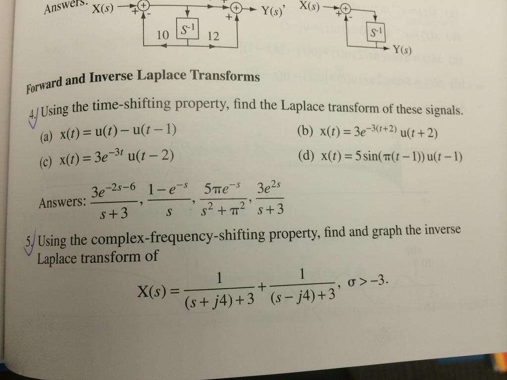
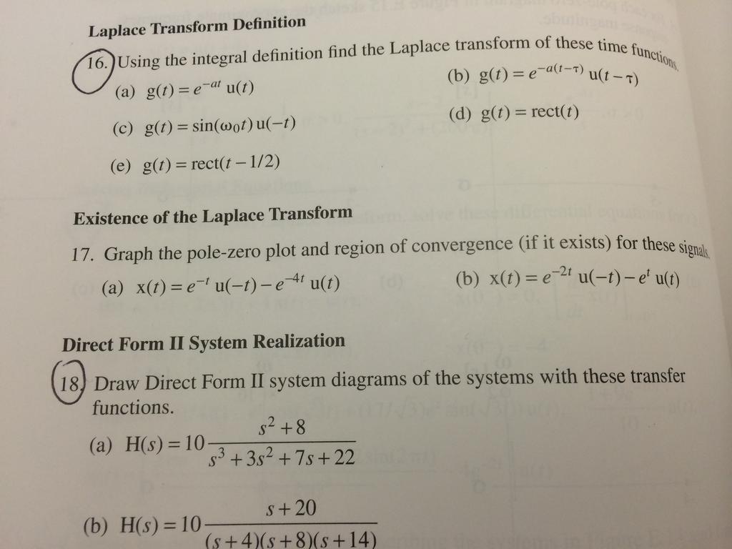
20 Direct Form II Realization! A very common form of transfer function is a ratio of two polynomials in s, ( ) = Y( s) X( s) = N b k s k=0 H s N k=0 k a k s k = b N s N + b N 1 s N b 1 s + b 0 a N s N + a N 1 s N a 1 s + a 0 1/13/11! M. J. Roberts - All Rights Reserved! 12!

21 The transfer function can be conceived as the product of two transfer functions, and Direct Form II Realization! H 1 H 2 ( s) = Y s 1 X s ( s) = Y s s Y 1 ( ) ( ) = 1 a N s N + a N 1 s N a 1 s + a 0 ( ) ( ) = b s N N + b N 1 s N b 1 s + b 0 1/13/11! M. J. Roberts - All Rights Reserved! 13!

22 From we get or X s H 1 ( s) = Y s 1 X s ( ) ( ) = 1 a N s N + a N 1 s N a 1 s + a 0 X( s) = a N s N + a N 1 s N a 1 s + a 0 Y 1 ( s) ( ) = a N s N Y 1 ( s) + a N 1 s N 1 Y 1 ( s) + + a 1 s Y 1 ( s) + a 0 Y 1 ( s) Rearranging s N Y 1 Direct Form II Realization! ( s) = 1 a N { X( s) a N 1 s N 1 Y 1 ( s) + + a 1 s Y 1 ( s) + a 0 Y 1 ( s) } 1/13/11! M. J. Roberts - All Rights Reserved! 14!

26 Inverse Laplace Transform! There is an inversion integral y( t) = 1 j2π σ + j Y( s)e st ds, s = σ + jω σ j for finding y( t) from Y( s), but it is rarely used in practice. Usually inverse Laplace transforms are found by using tables of standard functions and the properties of the Laplace transform. 1/13/11! M. J. Roberts - All Rights Reserved! 18!

27 If x t Existence of the Laplace Transform! Time Limited Signals! ( ) = 0 for t < t 0 and t > t 1 it is a time limited signal. If ( ) is also bounded for all t, the Laplace transform integral x t converges and the Laplace transform exists for all s. 1/13/11! M. J. Roberts - All Rights Reserved! 19!

28 Existence of the Laplace Transform! Let x( t) = rect ( t) = u( t +1/ 2) u( t 1/ 2). X s ( ) = rect t ( )e st dt = e st dt = e s/2 e s/2 s 1/2 1/2 = es/2 e s/2 s, All s 1/13/11! M. J. Roberts - All Rights Reserved! 20!

30 Existence of the Laplace Transform! Right- and Left-Sided Exponentials! ( ) = e αt u t t 0 x t Right-Sided! ( ), α x t Left-Sided! ( ) = eβt u t 0 t ( ), β 1/13/11! M. J. Roberts - All Rights Reserved! 22!

31 Existence of the Laplace Right-Sided Exponential! x( t) = e αt u( t t 0 ), α ( ) = e αt e st dt X s If Re s t 0 Transform! = e ( α σ )t e jωt dt ( ) = σ > α the asymptotic behavior of e ( α σ )t e jωt as t is to approach zero and the Laplace transform integral converges. t 0 1/13/11! M. J. Roberts - All Rights Reserved! 23!

32 Existence of the Laplace Left-Sided Exponential! x( t) = e βt u t 0 t ( ) = e βt e st dt X s ( ), β Transform! t 0 = e ( β σ )t e jωt dt t 0 If σ < β the asymptotic behavior of e ( β σ )t e jωt as t is to approach zero and the Laplace transform integral converges. 1/13/11! M. J. Roberts - All Rights Reserved! 24!

33 Existence of the Laplace Transform! The two conditions σ > α and σ < β define the region of convergence (ROC) for the Laplace transform of right- and left-sided signals. 1/13/11! M. J. Roberts - All Rights Reserved! 25!

34 Existence of the Laplace Transform! Any right-sided signal that grows no faster than an exponential in positive time and any left-sided signal that grows no faster than an exponential in negative time has a Laplace transform. ( ) = x r ( t) + x l ( t) where x r ( t) is the right-sided part and ( t) is the left-sided part and if x r ( t) < K r e αt and x l ( t) < K l e βt If x t x l and α and β are as small as possible, then the Laplace-transform integral converges and the Laplace transform exists for α < σ < β. Therefore if α < β the ROC is the region α < β. If α > β, there is no ROC and the Laplace transform does not exist. 1/13/11! M. J. Roberts - All Rights Reserved! 26!

35 Laplace Transform Pairs! The Laplace transform of g 1 G 1 ( s) = Ae αt u( t)e st dt ( t) = Ae αt u( t) is 0 = A e ( s α )t dt = A e ( α σ )t e jωt dt = A s α This function has a pole at s = α and the ROC is the region to the right of that point. The Laplace transform of g 2 ( t) = Ae βt u t G 2 0 ( ) is ( s) = Ae βt u( t)e st dt = A e ( β s)t dt = A e ( β σ )t e jωt dt = A s β 0 This function has a pole at s = β and the ROC is the region to the left of that point. 0 1/13/11! M. J. Roberts - All Rights Reserved! 27!

36 Region of Convergence! The following two Laplace transform pairs illustrate the importance of the region of convergence. e αt u t ( ) L 1 s + α, σ > α e αt L u( t) 1 s + α, σ < α The two time-domain functions are different but the algebraic expressions for their Laplace transforms are the same. Only the ROC s are different. 1/13/11! M. J. Roberts - All Rights Reserved! 28!

37 Region of Convergence! Some of the most common Laplace transform pairs! (There is more extensive table in the book.)! ramp t u( t) L ( ) = t u( t) L e αt u( t) L L δ ( t) 1, All σ u( t) L ( ) = t u( t) L ( ), σ > α e αt u( t) L 1/ s, σ > 0 1/ s 2, σ > 0 ramp t 1/ s + α 1/ s, σ < 0 1/ s 2, σ < 0 1/ s + α ( ), σ < α e αt sin( ω 0 t)u t e αt cos( ω 0 t)u t ( ) L ( ) L ω 0 ( s + α ) ω 0 s + α ( s + α ) ω 0, σ > α e αt sin( ω 0 t)u t, σ > α e αt cos( ω 0 t)u t ( ) L ( ) L ω 0 ( s + α ) ω 0 s + α ( s + α ) ω 0, σ < α, σ < α

41 Laplace Transform Example! Find the Laplace transform of ( ) = e t u( t) + e 2t u( t) x t e t u t e 2t u t ( ) L 1 s +1, σ > 1 ( ) L 1 s 2, σ < 2 e t u( t) + e 2t L u( t) 1 s +1 1 s 2, 1 < σ < 2 1/13/11! M. J. Roberts - All Rights Reserved! 30!

42 Laplace Transform Example! Find the inverse Laplace transform of The ROC tells us that right-sided signal and that a left-sided signal. X( s) = 4 s s 6, 3 < σ < 6 x t 4 must inverse transform into a s must inverse transform into s 6 ( ) = 4e 3t u( t) +10e 6t u( t) 1/13/11! M. J. Roberts - All Rights Reserved! 31!

43 Laplace Transform Example! Find the inverse Laplace transform of X( s) = 4 s s 6, σ > 6 The ROC tells us that both terms must inverse transform into a right-sided signal. ( ) = 4e 3t u( t) 10e 6t u( t) x t 1/13/11! M. J. Roberts - All Rights Reserved! 32!

44 Laplace Transform Example! Find the inverse Laplace transform of X( s) = 4 s s 6, σ < 3 The ROC tells us that both terms must inverse transform into a left-sided signal. ( ) = 4e 3t u( t) +10e 6t u( t) x t 1/13/11! M. J. Roberts - All Rights Reserved! 33!

45 MATLAB System Objects! A MATLAB system object is a special kind of variable in MATLAB that contains all the information about a system. It can be created with the tf command whose syntax is sys = tf(num,den) where num is a vector of numerator coefficients of powers of s, den is a vector of denominator coefficients of powers of s, both in descending order and sys is the system object. 1/13/11! M. J. Roberts - All Rights Reserved! 34!

46 MATLAB System Objects! For example, the transfer function H 1 ( s) = can be created by the commands s s 5 + 4s 4 + 7s 3 +15s s + 75»num = [1 0 4] ; den = [ ] ;»H1 = tf(num,den) ;»H1 Transfer function: s ^ s ^ s ^ s ^ s ^ s /13/11! M. J. Roberts - All Rights Reserved! 35!

47 Partial-Fraction Expansion! The inverse Laplace transform can always be found (in principle at least) by using the inversion integral. But that is rare in engineering practice. The most common type of Laplace-transform expression is a ratio of polynomials in s, G( s) = b s M M + b M 1 s M b 1 s + b 0 s N + a N 1 s N 1 + a 1 s + a 0 The denominator can be factored, putting it into the form, G s ( ) = b M s M + b M 1 s M b 1 s + b 0 ( s p 1 )( s p 2 ) s p N ( ) 1/13/11! M. J. Roberts - All Rights Reserved! 36!

48 Partial-Fraction Expansion! For now, assume that there are no repeated poles and that N > M, making the fraction proper in s. Then it is possible to write the expression in the partial fraction form, where G( s) = K 1 + K s p 1 s p 2 K N s p N b M s M + b M 1 s M 1 + b 1 s + b 0 = K 1 + K ( s p 1 )( s p 2 ) ( s p N ) s p 1 s p 2 The K s can be found be any convenient method. K N s p N 1/13/11! M. J. Roberts - All Rights Reserved! 37!

49 Partial-Fraction Expansion! Multiply both sides by s p 1 ( s p 1 ) b s M M + b M 1 s M b 1 s + b 0 ( s p 1 )( s p 2 ) ( s p N ) = K 1 + ( s p 1 ) + ( s p 1 ) K 2 + s p 2 K N s p N K 1 = b p M M M 1 + b M p b 1 p 1 + b 0 ( p 1 p 2 ) ( p 1 p N ) All the K s can be found by the same method and the inverse Laplace transform is then found by table look-up. 1/13/11! M. J. Roberts - All Rights Reserved! 38!

50 H( s) = Partial-Fraction Expansion! 10s s + 4 K 1 = s + 4 ( )( s + 9) = K 1 ( ) K 2 = s + 9 ( ) H( s) = 8 s s s ( s + 4) s + 9 s K 2 s + 9, σ > 4 ( ) 10s ( s + 4) s + 9 ( ) h( t) = ( 8e 4t +18e 9t )u( t) = s= 4 = s= 9 10s s s s + 4 8s s + 72 = s + 4 ( )( s + 9) = 40 s= 4 5 = 8 = 90 s= 9 5 = 18 = 10s s + 4 ( )( s + 9). Check. 1/13/11! M. J. Roberts - All Rights Reserved! 39!

51 Partial-Fraction Expansion! If the expression has a repeated pole of the form, ( ) = b M s M + b M 1 s M b 1 s + b 0 G s ( s p 1 ) 2 ( s p 3 ) ( s p N ) the partial fraction expansion is of the form, G( s) = K 12 K N ( s p 1 ) + K 11 + K s p 1 s p 3 s p N and K 12 can be found using the same method as before. But K 11 cannot be found using the same method. 1/13/11! M. J. Roberts - All Rights Reserved! 40!

52 Partial-Fraction Expansion! Instead K 11 can be found by using the more general formula K qk = 1 ( m k)! d m k ds m k ( ) ( s p ) m q H s s pq, k = 1,2,, m where m is the order of the qth pole, which applies to repeated poles of any order. If the expression is not a proper fraction in s the partialfraction method will not work. But it is always possible to synthetically divide the numerator by the denominator until the remainder is a proper fraction and then apply partial-fraction expansion. 1/13/11! M. J. Roberts - All Rights Reserved! 41!

53 Partial-Fraction Expansion! H( s) = 10s ( s + 4) 2 s + 9 Repeated Pole K 12 = s + 4 Using K qk = K 11 = ( ) = K 12 ( s + 4) + K 11 2 ( ) 2 10s ( s + 4) 2 ( s + 9) 1 d m k ( m k)! ds m k 1 ( 2 1)! d 2 1 s + 4 ds 2 1 s= 4 ( ) ( s p ) m q H s ( ) 2 H( s) s K 2 s + 9, σ > 4 = 40 5 = 8 s pq = d s 4 ds, k = 1,2,, m 10s s + 9 s 4 1/13/11! M. J. Roberts - All Rights Reserved! 42!

55 H( s) = H( s) = Partial-Fraction Expansion! 10s 2 s + 4 ( )( s + 9) 10s 2 s 2 +13s + 36, σ > 4, σ > 4 Improper in s Synthetic Division s 2 +13s s 2 H( s) = s s + 4 ( )( s + 9) h( t) = 10δ ( t) 162e 9t 32e 4t 10 10s s = 10 s s + 9 ( ) u t 130s 360, σ > 4 1/13/11! M. J. Roberts - All Rights Reserved! 44!

56 Inverse Laplace Transform Example! G( s) = G( s) = G( s) = 3 / 2 g t Method 1 s ( s 3) s 2 4s + 5 s ( s 3) s 2 + j ( ) ( )( s 2 j) ( ) / 4 ( ) / 4 s j s 2 + j ( ) = 3 2 e3t j 3 j s 2 j, σ < 2 4 e ( 2 j )t + 3 j 4 e 2+ j ( )t, σ < 2, σ < 2 u( t) 1/13/11! M. J. Roberts - All Rights Reserved! 45!

57 Inverse Laplace Transform Example! ( ) = 3 2 e3t j g t 4 e ( 2 j )t + 3 j 4 e 2+ j ( )t u( t) This looks like a function of time that is complex-valued. But, with the use of some trigonometric identities it can be put into the form ( ) = ( 3 / 2) e 2t cos( t) + 1/ 3 g t which has only real values. { ( )sin( t) e3t }u t ( ) 1/13/11! M. J. Roberts - All Rights Reserved! 46!

58 Inverse Laplace Transform Example! G( s) = G( s) = G( s) = 3 / 2 Method 2 s ( s 3) s 2 4s + 5 s ( s 3) s 2 + j ( ) ( )( s 2 j) ( ) / 4 ( ) / 4 s j s 2 + j 3 j s 2 j, σ < 2, σ < 2, σ < 2 Getting a common denominator and simplifying G( s) = 3 / 2 s s 10 s 2 4s + 5 = 3 / 2 s s 5 / 3 ( s 2) 2 + 1, σ < 2 1/13/11! M. J. Roberts - All Rights Reserved! 47!

59 Inverse Laplace Transform Example! Method 2 G( s) = 3 / 2 s s 5 / 3 ( s 2) 2 +1, σ < 2 The denominator of the second term has the form of the Laplace transform of a damped cosine or damped sine but the numerator is not yet in the correct form. But by adding and subtracting the correct expression from that term and factoring we can put it into the form G( s) = 3 / 2 s s 2 ( s 2) / 3 s 2 ( ) 2 +1, σ < 2 1/13/11! M. J. Roberts - All Rights Reserved! 48!

60 Inverse Laplace Transform Example! Method 2 G( s) = 3 / 2 s 3 3 s 2 2 ( s 2) / 3 ( s 2) 2, σ < 2 +1 This can now be directly inverse Laplace transformed into g( t) = ( 3 / 2) { e 2t cos( t) + ( 1/ 3)sin( t) e3t }u( t) which is the same as the previous result. 1/13/11! M. J. Roberts - All Rights Reserved! 49!

61 Inverse Laplace Transform Example! Method 3 When we have a pair of poles p 2 and p 3 that are complex conjugates we can convert the form G( s) = A s 3 + K 2 + K 3 s p 2 s p 3 ( ) K 3 p 2 K 2 p 3 into the form G( s) = A s 3 + s K 2 + K 3 = A s 2 ( p 1 + p 2 )s + p 1 p 2 s 3 + Bs + C s 2 ( p 1 + p 2 )s + p 1 p 2 In this example we can find the constants A, B and C by realizing that G( s) = s ( s 3) ( s 2 4s + 5) A s 3 + Bs + C s 2 4s + 5, σ < 2 is not just an equation, it is an identity. That means it must be an equality for any value of s. 1/13/11! M. J. Roberts - All Rights Reserved! 50!

62 Inverse Laplace Transform Example! Method 3 A can be found as before to be 3 / 2. Letting s = 0, the identity becomes 0 3 / C and C = 5 / 2. Then, letting 5 s = 1, and solving we get B = 3 / 2. Now G( s) = 3 / 2 s 3 + ( 3 / 2)s + 5 / 2, σ < 2 s 2 4s + 5 or G( s) = 3 / 2 s 3 3 s 5 / 3 2 s 2 4s + 5, σ < 2 This is the same as a result in Method 2 and the rest of the solution is also the same. The advantage of this method is that all the numbers are real. 1/13/11! M. J. Roberts - All Rights Reserved! 51!

63 Use of MATLAB in Partial Fraction Expansion! MATLAB has a function residue that can be very helpful in partial fraction expansion. Its syntax is [r,p,k] = residue(b,a) where b is a vector of coefficients of descending powers of s in the numerator of the expression and a is a vector of coefficients of descending powers of s in the denominator of the expression, r is a vector of residues, p is a vector of finite pole locations and k is a vector of so-called direct terms which result when the degree of the numerator is equal to or greater than the degree of the denominator. For our purposes, residues are simply the numerators in the partial-fraction expansion. 1/13/11! M. J. Roberts - All Rights Reserved! 52!

64 Let g t and h t Laplace Transform Properties! L ( ) and h( t) form the transform pairs, g( t) G( s) L ( ) H( s) with ROC's, ROC G and ROC H respectively. Linearity L α g( t) + β h( t) α G s ( ) + β H( s) ROC ROC G ROC H L Time Shifting g( t t 0 ) G( s)e st 0 s-domain Shift ROC = ROC G ( ) L ( ) e s0t g t G s s 0 ROC = ROC G shifted by s 0, (s is in ROC if s s 0 is in ROC G ) 1/13/11! M. J. Roberts - All Rights Reserved! 53!

65 Laplace Transform Properties! Time Scaling Time Differentiation s-domain Differentiation ( ) L g at ( ) ( 1/ a )G s / a ROC = ROC G scaled by a (s is in ROC if s / a is in ROC G ) d dt g( t) L ROC ROC G t g t ( ) L sg( s) d ds G( s) ROC = ROC G 1/13/11! M. J. Roberts - All Rights Reserved! 54!

66 Laplace Transform Properties! Convolution in Time Time Integration g( t) h t ( ) L G( s)h( s) ROC ROC G ROC H t L g( τ )dτ G( s) / s ( ) ROC ROC G σ > 0 If g( t) = 0, t < 0 and there are no impulses or higher-order singularities at t = 0 then Initial Value Theorem: g( 0 + ) = lim sg s s Final Value Theorem: lim g t t ( ) = lim ( ) s 0 sg s ( ) if lim t g t ( ) exists 1/13/11! M. J. Roberts - All Rights Reserved! 55!

67 Laplace Transform Properties! Final Value Theorem ( ) = lim limg t sg s t s 0 This theorem only applies if the limit lim g t t It is possible for the limit lim sg s s 0 limit lim g t t ( ) does not exist. For example x( t) = cos ω 0 t ( ) L ( ) ( ) actually exists. ( ) to exist even though the X( s) = s lim s X s s 0 ( ) 2 = lim s 0 s 2 + ω = but lim cos ω 0 t t ( ) does not exist. s s 2 + ω 0 2 1/13/11! M. J. Roberts - All Rights Reserved! 56!

68 Laplace Transform Properties! Final Value Theorem! ( ) if all the ( ) lie in the open left half of the s plane. Be sure ( ) must ( ) could have a single The final value theorem applies to a function G s poles of sg s to notice that this does not say that all the poles of G s lie in the open left half of the s plane. G s pole at s = 0 and the final value theorem would still apply. 1/13/11! M. J. Roberts - All Rights Reserved! 57!

69 Use of Laplace Transform Properties! ( ) = u( t) u( t a) and L ( ) L ( ) L ( ) Find the Laplace transforms of x t x( 2t) = u( 2t) u( 2t a). From the table u t Then, using the time-shifting property u t a Using the linearity property u( t) u t a Using the time-scaling property L u( 2t) u( 2t a) e as s s s/2 = 1 / s, σ > 0. e as / s, σ > 0. ( 1 e as ) / s, σ > 0. 1 e as/2 s, σ > 0 1/13/11! M. J. Roberts - All Rights Reserved! 58!

71 Use of Laplace Transform Properties! Use the s-domain differentiation property and ( ) L u t 1 / s, σ > 0 to find the inverse Laplace transform of 1 / s 2. The s-domain differentiation property is t g t ( ) L d ( ds G( s) ). Then t u t ( ) L d ds 1 s = 1. Then using the linearity property 2 s t u t ( ) L 1 s. 2 1/13/11! M. J. Roberts - All Rights Reserved! 59!

72 The Unilateral Laplace Transform! In most practical signal and system analysis using the Laplace transform a modified form of the transform, called the unilateral Laplace transform, is used. The unilateral Laplace transform is defined by G s ( ) = g t 0 ( )e st dt. The only difference between this version and the previous definition is the change of the lower integration limit from to 0. With this definition, all the Laplace transforms of causal functions are the same as before with the same ROC, the region of the s plane to the right of all the finite poles. 1/13/11! M. J. Roberts - All Rights Reserved! 60!

73 The Unilateral Laplace Transform! The unilateral Laplace transform integral excludes negative time. If a function has non-zero behavior in negative time its unilateral and bilateral transforms will be different. Also functions with the same positive time behavior but different negative time behavior will have the same unilateral Laplace transform. Therefore, to avoid ambiguity and confusion, the unilateral Laplace transform should only be used in analysis of causal signals and systems. This is a limitation but in most practical analysis this limitation is not significant and the unilateral Laplace transform actually has advantages. 1/13/11! M. J. Roberts - All Rights Reserved! 61!

74 The Unilateral Laplace Transform! The main advantage of the unilateral Laplace transform is that the ROC is simpler than for the bilateral Laplace transform and, in most practical analysis, involved consideration of the ROC is unnecessary. The inverse Laplace transform is unchanged. It is g( t) = 1 j2π σ + j σ j G( s)e + st ds 1/13/11! M. J. Roberts - All Rights Reserved! 62!

75 The Unilateral Laplace Transform! Some of the properties of the unilateral Laplace transform are different from the bilateral Laplace transform. Time-Shifting L g( t t 0 ) G( s)e 0, t 0 > 0 Time Scaling L g( at) ( 1 / a )G s / a First Time Derivative Nth Time Derivative Time Integration d N dt N t 0 d dt g t ( ) L ( g( t) L ) sg( s) g( 0 ) s N G s L g( τ )dτ G( s) / s ( ), a > 0 N d ( ) n 1 s N n n=1 dt n 1 ( g( t) ) t =0 1/13/11! M. J. Roberts - All Rights Reserved! 63!

76 The Unilateral Laplace Transform! The time shifting property applies only for shifts to the right because a shift to the left could cause a signal to become non-causal. For the same reason scaling in time must only be done with positive scaling coefficients so that time is not reversed producing an anti-causal function. The derivative property must now take into account the initial value of the function at time t = 0 and the integral property applies only to functional behavior after time t = 0. Since the unilateral and bilateral Laplace transforms are the same for causal functions, the bilateral table of transform pairs can be used for causal functions. 1/13/11! M. J. Roberts - All Rights Reserved! 64!

77 The Unilateral Laplace Transform! The Laplace transform was developed for the solution of differential equations and the unilateral form is especially well suited for solving differential equations with initial conditions. For example, d 2 dt 2 ( ) x t + 7 d dt with initial conditions x 0 ( ) x t ( ) = 2 and d dt + 12 x( t) = 0 ( x( t) ) t =0 = 4. Laplace transforming both sides of the equation, using the new derivative property for unilateral Laplace transforms, s 2 X( s) s x( 0 ) d dt ( ) ( x( t) ) t =0 + 7 s X( s) x X s ( ) = 0 1/13/11! M. J. Roberts - All Rights Reserved! 65!

78 The Unilateral Laplace Transform! Solving for X( s) or X( s) = x t =2 =2 = 4 s x( 0 ) + 7x( 0 ) + d ( x( t) ) dt t =0 s 2 + 7s s + 10 s 2 + 7s + 12 = 4 s The inverse transform yields s + 4 ( ). This solution solves the differential equation X( s) = ( )u t ( ) = 4e 3t 2e 4t with the given initial conditions. 1/13/11! M. J. Roberts - All Rights Reserved! 66!

79 Pole-Zero Diagrams and Frequency Response! If the transfer function of a stable system is H(s), the frequency response is H(jω). The most common type of transfer function is of the form, H s Therefore H(jω) is H jω ( ) = A s z 1 ( ) s z 2 ( s p 1 ) s p 2 ( ) = A jω z 1 ( ) s z M ( ) s p N ( ) jω z 2 ( jω p 1 ) jω p 2 ( ) ( ) ( ) jω z M ( ) jω p N ( ) ( ) 1/13/11! M. J. Roberts - All Rights Reserved! 67!

80 Let H( s) = 3s s + 3. H( jω ) = 3 jω jω + 3 The numerator jω and the denominator jω + 3 can be conceived as vectors in the s plane. H( jω ) = 3 Pole-Zero Diagrams and Frequency Response! jω jω + 3 H jω ( ) = 3 =0 + jω ( jω + 3 ) 1/13/11! M. J. Roberts - All Rights Reserved! 68!

81 Pole-Zero Diagrams and Frequency Response! lim ω 0 H( jω ) = lim 3 ω 0 jω jω + 3 = 0 lim ω 0 + H( jω ) = lim 3 ω 0 + jω jω + 3 = 0 lim H( jω ) = lim 3 ω ω jω jω + 3 = 3 lim H( jω ) = lim 3 ω + ω + jω jω + 3 = 3 1/13/11! M. J. Roberts - All Rights Reserved! 69!

82 Pole-Zero Diagrams and Frequency Response! lim H ( jω ) = π ω = π 2 lim H ( jω ) = π + ω = π 2 lim H jω ω ( ) = π 2 π 2 = 0 lim H jω ω + ( ) = π 2 π 2 = 0 1/13/11! M. J. Roberts - All Rights Reserved! 70!

91 Homework 3. Due date: 09/16/2016

The Laplace Transform

The Laplace Transform Generalizing the Fourier Transform The CTFT expresses a time-domain signal as a linear combination of complex sinusoids of the form e jωt. In the generalization of the CTFT to the