The construction and use of a phase diagram to investigate the properties of a dynamic system

Transcription

1 File: Phase.doc/pdf The construction and use of a phase diagram to investigate the properties of a dynamic system 1. Introduction Many economic or biological-economic models can be represented as dynamic systems of differential equations and associated measurement equations. The differential equations contain information about the equilibrium (or equilibria) of the system being investigated, the stability properties of that equilibrium, and the dynamics of the adjustment processes implicit in that system. Both this equilibrium and dynamic adjustment information can be compactly represented in a visual way by means of a phase diagram of the system. In this document, the construction and interpretation of phase diagrams is explained. The computer package Maple is used to construct two example of a phase diagram. Although it will be convenient for you to have access to Maple and to replicate these example yourself, that is not necessary for what follows. If you do not have access to Maple, a Word document copy of each of the Maple files is available from the Additional Materials pages. Moreover, in some simple cases at least, it should be possible for you to construct an approximation to an actual phase diagram using pen, paper and a little bit of simple algebra. The first example we shall use is the simple open access fishery model examined in the text of Chapter 17. The bioeconomic system in question is laid out in Table 17.8, Appendix 17.1, of the main text. You should look at the column labelled Continuous-time model. Of the two equations at the foot of the table under the heading FISHERY EFFORT DYNAMICS, it is the former the open-access entry rule which is applicable in this case. For convenience, we lay out the equations from that table which are relevant for our present purposes in Table 1 below. There are some minor changes in notation from Table 17.8 which should require no further explanation. 1

2 Table 1 The continuous-time version of the open access fishery model (with assumed functional forms) Fishery production function (1) H = ees Net (of harvest) growth of fish stock ds S (2) G(S) g 1 S S - H MAX Fishery profit (3) NB = B - C = PeES we Open access entry rule (4) de = (NB) Substituting equation (1) into equation (2), and equation (3) into equation (4), we obtain the following dynamic system consisting of two differential equations. ds S gs 1- ees S (5) MAX de δ PeES we (6) Note two points: Equations (5) and (6) are two differential equations in two variables, stock (S) and effort (E). All other terms in the two differential equations are parameters, baseline values of which are specified in the text. The two (implicit) measurement equations are H = ees (defining the fishery harvest) and NB = B - C = PeES we (defining the industry s net benefit, or profit). These allow us to compute the values of associated variables of interest once the solution values for S and E have been obtained. 2

3 2. Equilibrium solution The variable S will be in equilibrium for all combinations of S and E which satisfy ds/ = 0 in equation (5). That is, when S 0 gs 1- ees S (7) MAX By rearranging (7) to give S as a function of E, this yields SMAX(g ee) S (8) g The variable E will be in equilibrium for all combinations of S and E which satisfy de/ = 0 in equation (6). That is, when 0 δ PeES we (9) which written again in the form of S as a function of E - can be simplified to w S (10) Pe An equilibrium solution for the dynamic system given by Equations (5) and (6) consists of a pair of values for S and E at which the rates of change of S and E over time are simultaneously zero (i.e. ds/ = 0 and de/ = 0). That is, a solution will be one in which equations (7) and (9) hold together. To obtain a numerical solution, particular parameter values are required. With our baseline parameter values g0.15 S MAX 1 e0.015 P w0.6 the two equations that must be satisfied simultaneously are : S 1 0.1E (11) which follows from ds S (g ee) 0 S MAX g and 3

4 S 0.2 (12) which follows from de 0 S w Pe Solving (11) and (12) together gives S* = 0.2 and E* = 8. These two equilibrium relationships can be expressed graphically as shown in Figure 1 (which corresponds to Figure 17.6 in the textbook). Figure 1 ds S 0 S MAX (g ee) g S 1 0.1E de 0 S w Pe S 0.2 S* E* 4

5 3. System behaviour out of equilibrium We next attempt to establish the dynamic paths of E and S whenever {E t, S t } {E*, S*}. To do so, we consider the following questions: In which direction does E move when E is not in equilibrium? In which direction does S move when S is not in equilibrium? Combining the information from the answers to these two questions gives us qualitative information about the dynamic behaviour of the system when out of equilibrium. In which direction does E move when E is not in equilibrium? From Equation (6) it can be seen that if S > 0.2 then de/ > 0. 1 Hence any point on the phase diagram above the line S = 0.2 must be one in which de/ is positive, and so E is increasing over time. Conversely, if S < 0.2 then de/ < 0. Hence any point on the phase diagram below the line S = 0.2 must be one in which de/ is negative, and so E is decreasing over time. This reasoning divides the space on the phase plan diagram into two sub-spaces, with E increasing in one and falling in the other. In which direction does S move when S is not in equilibrium? From Equation (5) it can be seen that if S > (1-0.1E) then ds/ < 0. 2 Hence any point on the phase diagram to the right of the line S = 1-0.1E must be one in which ds/ is negative, and so S is decreasing over time. Conversely, if S < (1-0.1E) then ds/ > 0. Hence any point on the phase diagram to the left of the line S = 1-0.1E must be one in which ds/ is 1 Take Equation (6) and divide both sides by E. Then substitute in parameter values for P, e de ( ) and w on the right-hand side. Simplifying the resulting expression gives 20S 4. E Hence if (20S 4) > 0, then (de/)/e >0. But then dividing each of these inequalities by 20, it follows that if (S 0.2) > 0 then (de/)/20e > 0, which in turn implies that de/ > 0. 2 Take Equation (5) and divide both sides by S. Then substitute in parameter values for g, e and S MAX on the right-hand side. Simplifying the resulting expression gives ds ( ) 0.15(1 S) 0.015E. You should be able to deduce the necessary inequalities from S this result. 5

6 positive, and so S is rising over time. This reasoning also divides the space on the phase plan diagram into two sub-spaces, with S increasing in one and falling in the other. This information is put together in Figure 2. The diagram is effectively divided into four quadrants by the two equilibrium lines. In each quadrant is a direction indicator shown by two combined arrows, one pointing horizontally and the other vertically. For example in the quadrant above the S = 0.2 line and to the left of the S = 1 0.1E line the direction indicator is shown by the symbol The directions of each of the arrowheads show the movement of E and S. Specifically, E (the variable on the horizontal axis) is rising, and S (the variable on the vertical axis) is also rising. At different points in the space spanned by this quadrant the relative magnitudes of the forces changing E and S will differ. For example, it can be calculated from the two equations (5) and (6) (although this is not done so here) that at a point towards the bottom right of this quadrant such as the point {E, S} = {2, 0.25} that the absolute size of the upward movement of S is greater than the size of the increase in E. So, if the direction indicator at that point was drawn to a correct (relative) scale it would resemble and the vector of combined forces would be represented by the dashed line below In fact, we could calculate the dotted arrow vector of combined forces for every point on the space of the diagram. Figure 3 (identical to Figure 17.6: Phase-plane analysis of stock and effort dynamic paths for the illustrative model in the text) shows what this would look like (but using red solid rather than dashed arrows). Figure 3 has been obtained by using the 6

7 Maple package. The required code is shown in Chapter17.mw (and is copied in a Word file as Chapter17mw.doc). Figure 2 ds S 0 S MAX (g ee) g S 1 0.1E de 0 S w Pe S 0.2 7

8 Finally, note that Figure 3 (or equivalently Figure 17.6) shows one particular trajectory as a blue line. This line describes the dynamic adjustment process for the system from an initial point at which S is just below 1 and E is just larger than zero. The adjustment path through time is shown by the curved blue line. We begin at the top left point of the curved adjustment path. As time passes, stock falls and effort rises the adjustment path heads south-eastwards. After some time, the stock continues to fall but so too does effort the adjustment path follows a south-west direction. Looking at the path as a whole, we see that it converges through a series of diminishing cycles on the steady state equilibrium. As the main text pointed out, the (open access fishery model) examined here, in conjunction with the particular baselines parameter values being assumed, has strong stability properties: irrespective of where stock and effort happen to be the adjustment paths will lead to the unique steady state equilibrium, albeit through a damped, oscillatory adjustment process. 8

9 Figure 3: Phase plane dynamics of the open access model 9

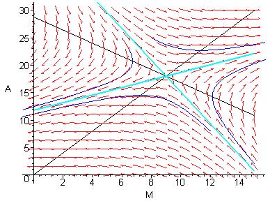
10 4. Dynamics of the Local Stock Pollution Model of Chapter 16. The second example we investigate is the local stock pollution model discussed in Chapter 16. The dynamic system was defined as the two differential equations 16.9 and 16.25a. That is: da = M 0.5A (16.9b) dm = 0.6M 0.5A 14.4 (16.25b) These two equations determine the dynamics of the state variable (A t, the pollution stock) and the instrument or control variable (M t, the flow of emissions). In steady state, variables are unchanging through time, so da/ A =0 and dm/ M =0. Imposing these values, and solving the two resulting equations yields M * = 9 and A * = 18. This steady state solution is shown in the phase plane diagram, Figure 16.5 by the intersection of the two lines labelled A =0 and M =0 (which are here A = 2M and A = (-0.6/0.5)M from 16.9 / and / ). Figure 16.5 is reproduced below for convenience. Next, we establish in which direction A and M will move over time from any pair of initial values {A 0, M 0 }. The two lines A =0 and M =0 (known as isoclines) divide the space into four quadrants. Above the line A =0, A > 2M, decay exceeds emissions flows, and so A is falling. Conversely below the line A =0, A < 2M, decay is less than emissions flows, and so A is rising. These movements are shown by the downward facing directional arrows in the two quadrants labelled a and b, and by upward facing directional arrows in the two quadrants labelled c and d. Above the line M =0, 0.6M > A, and so from Equation 16.25b we see that M is rising. Below the line M =0, 0.6M < A, and so M is falling. These movements are shown by the leftward facing directional arrows in the two quadrants labelled a and d, and by rightward facing directional arrows in the two quadrants labelled b and c. 10

11 Taking these results together we obtain the pairs of direction indicators for movements in A and M for each of the four quadrants when the system is not in steady state. The curved lines illustrate four paths that the variables would take from particular initial values. Thus, for example, if the initial values lie in quadrant d with M = 15 and A = 2, the differential equations which determine A and M would at first cause M to fall and A to rise over time. As this trajectory crosses the M =0 isocline into quadrant c, A will continue to rise but now M will also rise too. Left alone, the system would not reach the steady state optimal solution, diverging ever further from it as time passes. Inspection of the other three trajectories shows that these also fail to attain the steady state optimum, and eventually diverge ever further from it. Inspection of Figure 16.5 shows two other lines, of a kind which we have not come across before. These two dotted lines sometimes called separatrices - both pass through the steady-state equilibrium of the system. One of them known as the stable arm is annotated with arrows which point towards the equilibrium The other known as the unstable arm is annotated with arrows which point away from the equilibrium. Further inspection shows that there are only two paths which lead to the steady state equilibrium. These two paths consist of movements along the stable arm, either in a southeasterly direction or in a north-westerly direction. Now suppose that the policy maker has determined that the steady-state equilibrium is an optimal target. Then, for any dynamic process such as this, the only way of reaching that optimum is for the policy maker to control M so as to reach the stable arm, and then to adjust M appropriately along the stable arm until the optimal point is reached. A system with the dynamic properties shown in Figure 16.5 exhibits what is known as a saddle point equilibrium. 11

12 Figure 16.5 Steady state solution and dynamics of the waste accumulation and disposal model. b A 0 * A 18 a c d M 0 * M 9 12

13 5. A method of calculating the separatrices of the dynamic system How can we obtain the stable and unstable arms of the dynamic system? We will need to make use of a little matrix algebra, and the concepts of eigenvalues and eigenvectors. The first step is to write our two equation differential equation system in the special matrix form of a linear system 3 x Ax b where M x A M x A 0.6 A b 0 For the moment, we ignore the vector of constant terms b. Our next step is to obtain the eigenvalues and eigenvectors of the matrix A. The eigenvalues of A (also known as the characteristic roots of A) are the values of which satisfy the equation det(a - I) = 0 (13) where the symbol det denotes the determinant of the matrix in parentheses which follows it, and I is the identity matrix. The eigenvectors of the matrix are the solutions to (13) for each particular eigenvalue. 4 These can be easily found using a mathematical package. For example, using the following Maple code (in the Maple file Stock pollution 1.mws), we obtain the two eigenvalues of A as r 1 = and r 2 = Corresponding to the eigenvalue r 1 = is the eigenvector v and corresponding to the eigenvalue r 2 = is the eigenvector v The order in which the equations appear is arbitrary. Our results would be identical for the other ordering. 4 For a simple treatment of eigenvectors and eigenvalues, see Chiang (1984), chapter

14 The gradients of these two eigenvectors determine the directions of the two separatrices of the system: the unstable arm (v 1 in this case) and the stable arm (v 2 in this case). These separatrices must pass through the equilibrium (or fixed point of the system at A* = 18 and M* = 9. They are shown in Figure 16.5 as the two dotted blue lines, with the stable (unstable) arm showing arrows pointing to (away from) the fixed point. The eigenvalues of the system determine the nature of the equilibrium of the system. Specifically for a two-equation system, the possibilities include 5 1. If the eigenvalues are real numbers, are distinct, and are of the same sign, then the equilibrium is stable (with both separatrices being stable arms) 2. If the eigenvalues are real numbers, are distinct, and are of opposite signs, then the system has an unstable saddle point equilibrium (with one separatrix being the stable arm and the other the unstable arm) 3. If the eigenvalues are complex numbers, then (depending on the particular values of r 1 and r 2 ) the system will have one of the following properties: a stable equilibrium with the convergence paths spiralling inwards towards the fixed point an unstable equilibrium with dynamic adjustment paths diverging in a spiral manner outwards and away from the fixed point dynamic paths taking the form of closed circles or ellipses (with either clockwise or anticlockwise direction), and so neither converging on nor diverging from the centre of the closed curve. Clearly, in the example of the local stock-pollution model that we have just been investigating, the eigenvalues of A ( r 1 = and r 2 = ) fall into category 2 above, that of an unstable saddle point equilibrium (as we discovered earlier by inspection of the phase diagram for the system). We shall see later in this document that the open access model falls into (the first bullet pointed case of) category 3. 5 See Shone (2002) Chapter 4 for more details and a complete catalogue of all possible forms of equilibria. 14

15 The text below shows the Maple code used to generate the phase plane diagram which underlies Figure The first line defines two ratios of constant numbers (actually ratios of elements of the matrix of eigenvectors) which are used lower down in the code to draw lines representing the two separatrices. Our code rather inelegantly manipulates the locations of the stable and unstable arms so that they not only have the correct directions but also pass through the fixed (equilibrium) point of the system. (See the code beginning lines92.) At the end of the code itself, we have copied the phase plane diagram as it constructed by Maple from this code. > rat1:= / ;rat2:= / ; rat1 := The differential equations defined: rat2 := > eqs92:={diff(m(t),t)=0.5*a(t)+0.6*m(t)-14.4, diff(a(t),t)=m(t)-0.5*a(t)}; d d eqs92 := { M( t) 0.5 A( t) 0.6 M( t) 14.4, A( t) M( t) 0.5 A( t )} >init92:=[[m(0)=8,a(0)=25],[m(0)=12,a(0)=8],[m(0)=6,a(0)=25],[ M(0)=15,A(0)=2]]; init92 := [[ M( 0)8, A( 0) 25 ], [ M( 0)12, A( 0) 8 ], [ M( 0)6, A( 0) 25], [ M( 0)15, A( 0) 2 ]] >curves92:=deplot(eqs92,[m(t),a(t)],t=0..200,m=0..15,a=0..30,i nit92,stepsize=.2,arrows=thin,linecolour=blue,thickness=1): > lines92:=plot({(18-rat2*9)+( / )*m,(18- rat1*9)+( / )*m},m=0..15,a=0..30,colour=cyan, thickness=2): > lines93:=plot({(2*m), ((-0.6/0.5)*M+(14.4/0.5))}, M=0..15,A=0..30,colour=black): > display({curves92,lines93,lines92}); 15

16 16

17 6. Revisiting the open access model Finally, we return to our open access model. The two differential equations of the dynamic system are (see footnotes 1 and 2): ds (0.15(1 S) 0.015E)S de (20S 4)E This is a non-linear differential equation system. We have already seen that it has a fixed point (equilibrium) at (S = S* = 0.2, E = E* = 8). To examine the stability properties of the system near this equilibrium, we need to obtain a linear approximation to the non-linear system around the fixed point. Such an approximation can be obtained using Taylor series expansions. Thus, if we write the system as ds f (S,E) de g(s, E) a linear approximation to the non-linear system around the point (S = S*, E = E*) is given by ds f (S*,E*) f (S*,E*) S* (S S*) (E E*) S E de g(s*,e*) g(s*,e*) E* (S S*) (E E*) S E Then the matrix of coefficients A is formed as (the numerical values of ) the partial derivatives f (S*,E*) A S g(s*,e*) S f (S*,E*) E g(s*,e*) E From this matrix we may proceed as before, obtaining eigenvalues and eigenvectors to establish the system stability properties around the fixed point. The following Maple code obtains the eigenvalues of the linear approximation to this system around the point {S* = 0.2, E* = 8} > taylor((0.15*(1-s)-0.015*e)*s, s=s,2); ( S0.015 e) S ( S0.015 e ) ( ss ) O (( ss ) 2 ) > taylor((0.15*(1-s)-0.015*e)*s, e=e,2); 17

18 ( s0.015 E) s0.015 s ( ee ) > taylor((20*s-4)*e, s=s,2); ( 20 S4) e20 e ( ss ) > taylor((20*s-4)*e, e=e,2); ( 20 s4 ) E ( 20 s4 ) ( ee ) Obtaining numerical values of the partial derivatives: > * *8;-0.015*0.2;20*8;20*0.2-4; We have below labelled the A matrix as beta1: > beta1:=matrix([[-0.03, ], [160, 0]]); := > eigenvalues(beta1); I, I We see that the two eigenvalues are complex numbers of the form r α βi r 1 2 α βi with < 0 and >0. This configuration of roots corresponds to a stable equilibrium, converging (in terms of Figure 3) by means of a damped clockwise spiral to the fixed point equilibrium