Physics 351 Monday, January 22, 2018

Transcription

1 Physics 351 Monday, January 22, 2018

2 Phys 351 Work on this while you wait for your classmates to arrive: Show that the moment of inertia of a uniform solid sphere rotating about a diameter is I = 2 5 MR2. The integral is easiest in spherical polar coordinates, with the axis of rotation taken to be the z axis. Helpful hint: dv = r 2 dr d(cos θ) dφ. [For this problem, that form is simpler to use than the other form you may have seen, dv = r 2 dr sin θ dθ dφ But to account for the minus sign you then integrate from cos θ = 1 to cos θ = +1 instead of from θ = 0 to θ = π.]

3

4 Physics 351 Monday, January 22, 2018 Homework #1 due on Friday 1/26. Homework help sessions start Jan (Wed/Thu). After finishing up Friday s discussion of spherical polar coordinates, we ll spend the rest of this week on Ch 5 6. I m aiming to start Lagrangians by the end of Friday. You ve now read Chapters 1 6. The pace will calm down now, as we start the new material.

5 Taylor s Chapter 4 comment that in polar coordinates, a b = a r b r + a θ b θ + a φ b φ means that e.g. at one point on or near Earth s surface, you can set up an orthonormal local coordinate system and write ˆr = up unit vector ˆθ = south unit vector ˆφ = east unit vector Then I can write out the components of e.g. a force F and a displacement r in that orthonormal coordinate system and write e.g. Work = F r W = F up r up + F south r south + F east r east

6 z = r cos θ x = r sin θ cos φ y = r sin θ sin φ If I move dr up, and dθ south, and dφ east, what is my resulting displacement vector? d r = ˆrA + ˆθB + ˆφC What are A, B, and C? (All have dimensions of length.)

7 z = r cos θ x = r sin θ cos φ y = r sin θ sin φ If I move dr up, and dθ south, and dφ east, my displacement vector is d r = ˆr dr + ˆθ rdθ + ˆφ r sin θdφ (This is useful when computing the distance between two (nearby) terrestrial points, given their (latitude,longitude) geocodes.)

8

9

10

11 (You try it!)

12

13 (A central force exerted by Earth s center can have an up/down component but cannot have E/W or N/S components.)

14 (You can prove the converse as a future XC problem, if you wish.)

15 One point worth emphasizing from the end of Chapter 4 (Energy): For two particles interacting only with each other, U( r 1, r 2 ) = U( r 1 r 2 ) in this case, which implies U = U x 1 x 2 U = U y 1 y 2 F 2 = F 1 U = U z 1 z 2 Since there is no ext. force, this is just Newton #3: F12 = F 21 You know 3rd law momentum conservation Deep connection (Noether s theorem): translation invariance momentum conservation

16 Damped harmonic motion (b = linear drag coefficient from ch2): mẍ = kx bẋ let ω 0 = k/m let β = b/(2m) ẍ + 2βẋ + ω 2 0x = 0 This is a linear, 2nd order, homogeneous differential equation. Linear because x, ẋ, ẍ, etc. appear only as the first power, not e.g. ẋ 2, xẋ, x 2, sin(x), etc. More precisely, linear because we re applying a linear operator D to turn the variable x into the LHS: D = d2 dt 2 + 2β d dt + ω2 0 D[Ax 1 +Bx 2 ] = d2 dt 2 (Ax 1+Bx 2 ) + 2β d dt (Ax 1+Bx 2 ) + ω 2 0(Ax 1 +Bx 2 ) = Aẍ 1 + 2βAx 1 + Aω0x Bẍ 2 + 2βBx 2 + Bω0x 2 2 = AD[x 1 ] + BD[x 2 ]

17 The amazingly useful feature of linearity is that linearity permits us to use the superposition principle If we have two functions x 1 (t) and x 2 (t) that separately satisfy D[x 1 (t)] = 0 D[x 2 (t)] = 0 (where D is a linear operator) then a linear combination x 3 (t) = Ax 1 (t) + Bx 2 (t) will also satisfy D[x 3 (t)] = 0 So the superposition of several solutions is also a solution.

18 ẍ + 2βẋ + ω 2 0x = 0 is a linear, 2nd order, homogeneous differential equation. Second-order because the order of the highest derivative is 2. Any linear diff eq of order n has n independent solutions, i.e. general solution contains n arbitrary constants. Homogeneous because the RHS is zero. If the RHS is some f(t), we call this an inhomogeneous diff eq. We ll say this again later: The general solution to (inhomogeneous) D[x] = f(t) is the sum of any particular solution to D[x] = f(t) plus the general solution to D[x] = 0 We ll need that to study forced (or driven ) oscillations. Now back to our equation.

19 ẍ + 2βẋ + ω 2 0x = 0 Let s guess (!) a solution x(t) = Ae αt and plug it in: (α 2 + 2αβ + ω0) 2 Ae αt = 0 α = β ± β 2 ω0 2 So (except for the degenerate β = ω 0 case), we ve found our two independent solutions: x(t) = Ae βt e +Ωt + Be βt e Ωt where Ω = β 2 ω0 2. The most common case is weak damping ( underdamped ), where β < ω 0, so Ω 2 < 0. Then Ω = i ω0 2 β2 = iω 1 x(t) = e βt ( Ae iω 1t + Be iω 1t ) = Ce βt cos(ω 1 t + φ 0 ) If β = 0.2ω 0, then ω ω 0. If β = 0.1ω 0, then ω ω 0.

20 By suitable choice of A and B, we can ensure that x(t) is real, and that the arbitrary constants C and φ 0 are real. x(t) = e βt ( Ae iω1t + Be iω 1t ) = Ce βt cos(ω 1 t + φ 0 ) Digression: e iθ = cos θ + i sin θ cos θ = 1 2 (eiθ + e iθ ) sin θ = 1 2i (eiθ e iθ ) Re(z) = 1 2 (z + z ) Im(z) = 1 2i (z z ) By analogy, cosh θ = 1 2 (eθ + e θ ) sinh θ = 1 2 (eθ e θ ) So choosing A = 1 2 Ceiφ 0 and B = 1 2 Ce iφ 0 gives x(t) = Ce βt cos(ω 1 t + φ 0 ) where C and φ 0 are fixed by the initial conditions. ω 1 ( ω 0 ) and β are properties of the system. Quality factor Q = ω 0 /(2β).

21 x(t) = Ce βt cos(ω 1 t + φ 0 ) Q = ω 0 /(2β). energy(t) e 2βt = e ω 0t/Q = e 2πf 0t/Q = e 2πt/(QT 0) So after Q periods (t = QT 0 ), the energy has decreased by a factor e 2π Equivalently, Q 2π = energy stored in oscillator energy dissipated per cycle [First two Mathematica Manipulate[] demos.]

22 For the special case β = 0 ( no damping ), ω 1 = ω 0 : Ω = i ω0 2 β2 = i ω0 2 0 = iω 0 x(t) = Ae iω 0t + Be iω 0t = C cos(ω 0 t + φ 0 ) For the β > ω 0 strong damping ( overdamped ) case, Ω 2 > 0, Ω is real and nonzero: Ω = β 2 ω0 2. Then x(t) = Ae (β β 2 ω 2 0 )t + Be (β+ β 2 ω 2 0 )t The first term dominates the decay rate, since the second term decays away more quickly. Interestingly, in this overdamped regime, increasing β (more damping) actually makes the motion decay less quickly! Decay rate is largest at critical damping, Ω 2 = 0. Important for shock absorbers, indicator needles.

23 Critical damping (Ω 2 = 0): Our previous procedure now gives us only one solution: β ± β 2 ω 2 0 = β x(t) = Ae βt There must be a second solution to Let s try another lucky guess: ẍ + 2βẋ + β 2 x = 0 x = Bte βt ẋ = Be βt βbte βt ẍ = βbe βt βbe βt + β 2 Bte βt ẍ = 2βBe βt + β 2 Bte βt 2βẋ = 2βBe βt 2β 2 Bte βt β 2 x = β 2 Bte βt which add up to zero. So we have x(t) = (A + Bt)e βt

24 Rate of exponential decay (e.g. 1/τ) vs. damping constant β. Beyond critical damping, adding more damping does not make the motion decay more quickly!

25 Driven damped oscillations (why are we allowed to pretend, counterfactually, that the driving force is complex?) Let s guess a solution ẍ + 2βẋ + ω 2 0x = F 0 e iωt x(t) = Ce iωt ( ω 2 + 2iβω + ω 2 0) Ce iωt = F 0 e iωt C = ω 2 + 2iβω + ω0 2 ( ) F 0 x(t) = ω 2 + 2iβω + ω0 2 e iωt This is a particular solution to the inhomogeneous linear diff. eq. But we already know that where Ω = β 2 ω 2 0 F 0 D[x(t)] = F 0 e iωt D[e βt (Ae +Ωt + Be Ωt )] = 0

26 D[Ce iωt ] = F 0 e iωt D[e βt (Ae +Ωt + Be Ωt )] = 0 So then D[e βt (Ae +Ωt + Be Ωt ) + Ce iωt ] = F 0 e iωt General solution to (inhomogeneous) D[x] = f(t) is sum of any particular solution to plus the general solution to D[x] = 0 D[x] = f(t) (inhomogeneous) x(t) = e βt (Ae +Ωt + Be Ωt ) + Ce iωt (homogeneous) Notice that β and ω 0 (and Ω = β 2 ω0 2 ) depend only on the oscillator itself, not on the driving force or the initial conditions. C and ω are properties of the external driving force. A and B depend on initial conditions, but become irrelevant for t 1/β. (The A and B terms are called the transient response.)

27 For driving force F 0 e iωt, we found x(t) = e βt (Ae +Ωt + Be Ωt ) + Ce iωt Once the transients have died away (after Q periods of ω 0 ), with x(t) = Ce iωt F 0 C = ω 2 + 2iβω + ω0 2 If the driving force had been F 0 e iωt, we would have found with x(t) = Ce iωt C = ω 2 2iβω + ω0 2 Linear superposition lets us average these two solutions to get the response to real driving force F 0 cos(ωt). F 0

28 For driving force F 0 cos(ωt) = F 0 2 (e iωt + e iωt ), we get (after transients die out) F 0 /2 x(t) = ω 2 + 2iβω + ω0 2 e iωt F 0 /2 + ω 2 2iβω + ω0 2 e iωt which is the same as ( F 0 x(t) = Re ω 2 + 2iβω + ω0 2 e iωt ) which after some algebra is x(t) = A cos(ωt δ) with A = F 0 (ω 2 0 ω 2 ) 2 + 4β 2 ω 2 ( ) 2βω δ = arctan ω0 2 ω2 [Mathematica and physical demos]

29 For driving force F 0 cos(ωt), we found x(t) = e βt (Ae +Ωt + Be Ωt ) + A cos(ωt δ) with Ω = β 2 ω 2 0 = iω 1 A = F 0 (ω 2 0 ω 2 ) 2 + 4β 2 ω 2 ( ) 2βω δ = arctan ω0 2 ω2 The important point to remember (for the usual underdamped case) is that the transient response rings at ω 1 ω 0, which is close to the natural frequency, and decays away at rate β. But the long-term response is at the driving frequency ω, with an amplitude and phase that depend on ω ω 0.

30

31 Let s go back to the complex-number driving force For driving force F 0 e iωt, we found x(t) = e βt (Ae +Ωt + Be Ωt ) + Ce iωt Once the transients have died away (after Q periods of ω 0 ), x(t) = Ce iωt with F 0 C = ω 2 + 2iβω + ω0 2

32 Now suppose you have a more complicated driving force: ẍ + 2βẋ + ω 2 0x = F a e iωat + F b e iω bt Since D is linear, [ F a e iωat ] D ωa 2 + 2iβω a + ω0 2 = F a e iωat [ F b e iω ] bt D ωb 2 + 2iβω b + ω0 2 = F b e iω bt [ F a e iωat F b e iω ] bt D ωa 2 + 2iβω a + ω0 2 + ωb 2 + 2iβω b + ω0 2 = F a e iωat + F b e iω bt So the general solution is F a e iωat F b e iω bt x(t) = ωa 2 + 2iβω a + ω0 2 + ωb 2 + 2iβω b + ω0 2 + e βt (Ae +Ωt +Be Ωt ) where again the transient terms are irrelevant for t 1/β.

33 Now consider the more general case and suppose we re able to write ẍ + 2βẋ + ω 2 0x = f(t) f(t) = n F n e iωnt Then it s clear that the solution would be x(t) = (transient) + n ω 2 n + 2iβω n + ω 2 0 F n e iωnt If f(t) is periodic (period T 2π/ω), then Prof. Fourier tells us f(t) = + n= F n e inωt

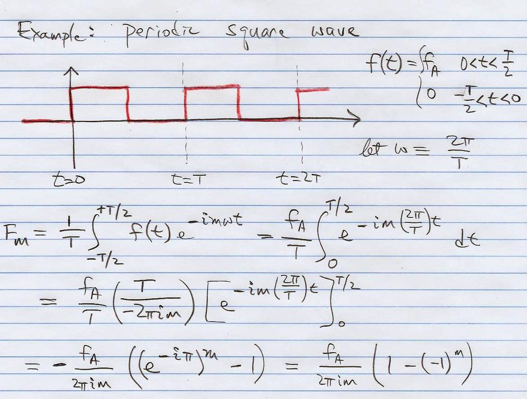
34 f(t) = + n= F n e inωt 1 T +T/2 T/2 f(t) e imωt dt = n F n T So the Fourier coefficient F m is +T/2 T/2 dt e i(n m)ωt = n F n δ mn = F m F m = 1 T +T/2 T/2 f(t)e imωt dt Note: for f(t) real, F m = F m, i.e. the negative-frequency coefficients are the complex conjugates of the corresponding positive-frequency coefficients.

35 f(t) = + n= with Fourier coefficient F n given by F n = 1 T +T/2 T/2 F n e inωt f(t)e inωt dt Exercise: use this complex-number Fourier formalism to find the Fourier series for a square wave f(t) of period T = 2π/ω, with f(t) = 0 for T/2 < t < 0 f(t) = A for 0 < t < T/2

36

37

38 f(t) = + n= F n e inωt F n = 1 T +T/2 T/2 f(t)e inωt dt Exercise: use this complex-number Fourier formalism to find the Fourier series for a triangle wave f(t) of period T = 2π/ω, with f(t) = 2At/T for T/2 < t < 0 f(t) = 2At/T for 0 < t < T/2 hint : te inωt dt = 1 + inωt (nω) 2 e inωt

39

40

41

42

43

44

45

46

47

48 Notice that the answer came out entirely real, even though we used complex exponentials. Also notice that this looks just like the result from the book using sines and cosines: f x n (t) = A n cos(nωt δ n ) A n = n same δ n (ω 2 0 n 2 ω 2 ) 2 +(2βnω) 2 and 2f A /(πn) is just f n. (sin vs. cos depends on chosen time offset of square wave.)

49 Physics 351 Monday, January 22, 2018 Homework #1 due on Friday 1/26. Homework help sessions start Jan (Wed/Thu). After finishing up Friday s discussion of spherical polar coordinates, we ll spend the rest of this week on Ch 5 6. I m aiming to start Lagrangians by the end of Friday. You ve now read Chapters 1 6. The pace will calm down now, as we start the new material.