Modeling and Simulation Revision IV D R. T A R E K A. T U T U N J I P H I L A D E L P H I A U N I V E R S I T Y, J O R D A N

Transcription

1 Modeling and Simulation Revision IV D R. T A R E K A. T U T U N J I P H I L A D E L P H I A U N I V E R S I T Y, J O R D A N

2 Modeling Modeling is the process of representing the behavior of a real system by a collection of mathematical equations and logic. Models are cause-and-effect structures they accept external information and process it with their logic and equations to produce one or more outputs. Parameter is a fixed-value unit of information Signal is a changing-unit of information Models can be text-based programming or block diagrams

3 Math Modelling Categories Static vs. dynamic Linear vs. nonlinear Time-invariant vs. time-variant SISO vs. MIMO Continuous vs. discrete Deterministic vs. stochastic

4 Static vs. Dynamic Models can be static or dynamic Static models produce no motion, fluid flow, or any other changes. 4 Example: Battery connected to resistor v = ir Dynamic models have energy transfer which results in power flow. This causes motion, or other phenomena that change in time. Example: Battery connected to resistor, inductor, and capacitor v Ri L di dt 1 C idt

5 Linear vs. Nonlinear Linear models follow the superposition principle The summation outputs from individual inputs will be equal to the output of the combined inputs Most systems are nonlinear in nature, but linear models can be used to approximate the nonlinear models at certain point.

6 Linear vs. Nonlinear Models Linear Systems Nonlinear Systems

7 Time-invariant vs. Time-variant The model parameters do not change in time-invariant models The model parameters change in time-variant models Example: Mass in rockets vary with time as the fuel is consumed. If the system parameters change with time, the system is time varying.

8 Time-invariant vs. variant Time-invariant F(t) = ma(t) g Time-variant F = m(t) a(t) g Where m is the mass, a is the acceleration, and g is the gravity Here, the mass varies with time. Therefore the model is time-varying

9 Linear Time-Invariant (LTI) LTI models are of great use in representing systems in many engineering applications. The appeal is its simplicity and mathematical structure. Although most actual systems are nonlinear and time varying Linear models are used to approximate around an operating point the nonlinear behavior Time-invariant models are used to approximate in short segments the system s time-varying behavior.

10 SISO vs. MIMO Single-Input Single-Output (SISO) models are somewhat easy to use. Transfer functions can be used to relate input to output. Multiple-Input Multiple-Output (MIMO) models involve combinations of inputs and outputs and are difficult to represent using transfer functions. MIMO models use State-Space equations

11 System States Transfer functions Concentrates on the input-output relationship only. Relates output-input to one-output only SISO It hides the details of the inner workings. State-Space Models States are introduced to get better insight into the systems behavior. These states are a collection of variables that summarize the present and past of a system Models can be used for MIMO models

12 SISO vs. MIMO Systems U(t) Transfer Function Y(t)

13 Continuous vs. discrete Continuous models have continuous-time as the dependent variable and therefore inputs-outputs take all possible values in a range Discrete models have discrete-time as the dependent variable and therefore inputs-outputs take on values at specified times only in a range

14 Continuous vs. discrete Continuous Models Discrete Models Differential equations Integration Laplace transforms Difference equations Summation Z-transforms

15 Deterministic vs. Stochastic Deterministic models are uniquely described by mathematical equations. Therefore, all past, present, and future values of the outputs are known precisely Stochastic models cannot be described mathematically with a high degree of accuracy. These models are based on the theory of probability

16 Block Diagrams Block diagram models consist of two fundamental objects: signal blocks and wires. A block is a processing element which operates on input signals and parameters to produce output signals A wire is to transmits a signal from its origination point (usually a block) to its termination point (usually another block). Block diagrams are suitable to represent multidisciplinary models that represent a physical phenomenon. Dr. Tarek A. Tutunji

17 Block Diagram Example [Ref.] Prof. Shetty

18 Block Diagrams Manipulation

19 Block Diagrams Manipulation

20 Block Diagrams: Direct Method Example Consider the transfer function: We can introduce s state variable, x(t), in order to separate the polynomials

21 State Equation The differential equation is: Put the needed integrator blocks: Add the required multipliers to obtain the state equation:

22 Output Equation Repeat the same procedure for the output equation: Connect the two sub-blocks

23 Block Diagram Modeling: Analogy Approach Physical laws are used to predict the behavior (both static and dynamic) of systems. Electrical engineering relies on Ohm s and Kirchoff s laws Mechanical engineering on Newton s law Electromagnetics on Faradays and Lenz s laws Fluids on continuity and Bernoulli s law Based on electrical analogies, we can derive the fundamental equations of systems in five disciplines of engineering: Electrical, Mechanical, Electromagnetic, Fluid, and Thermal. By using this analogy method to first derive the fundamental relationships in a system, the equations then can be represented in block diagram form, allowing secondary and nonlinear effects to be added. This two-step approach is especially useful when modeling large coupled systems using block diagrams.

24 Power and Energy Variables: Effort & Flow [Ref.] Raul Longoria

25 Transitional Mechanical Systems Mechanical movements in a straight line (i.e. linear motion) are called transitional Force displacement Basic Blocks are: Dampers, Masses, and Springs Springs represent the stiffness of the system F kx Dampers (or dashpots) represent the forces opposing to the motion (i.e. friction) F cv velocity Masses represent the inertia F ma mass acceleration Dr. Tarek A. Tutunji

26 Transitional Mechanical Systems Equations for mechanical systems are based on Newton Laws Free body diagram Spring Mass Force Damper ma F - kx - c dx dt Dr. Tarek A. Tutunji

27 Example: Mass-Spring-Damper Note: D is Differentiation 1/D is Integration

28 Example: Two-Mass Mechanical System [Ref.] Prof. Shetty

29 Example: Two-Mass Mechanical System

30 Example: Mechanical Model Consider a two carriage train system x1 x2 Force Mass 1 k(x1-x2) k(x1-x2) Mass 2 c v1 m m 1 2 x x 1 2 f - k(x k(x x 2 x2 ) - cx ) - cx 2 1 c v2

31 Example continued Taking the Laplace transform of the equations gives m s m 1 2 s 2 2 X X 1 2 (s) (s) F(s) - k(x k(x 1 (s) - 1 (s) - X 2 X 2 (s)) (s)) - csx - csx 2 (s) 1 (s) Note: Laplace transforms the time domain problem into s-domain (i.e. frequency) L L x(t) X(s) x(t) sx(s) 0 e st x(t)dt

32 Example continued Manipulating the previous two equations, gives the following transfer function (with F as input and V1 as output) V 1 (s) F(s) m m 1 2 s 3 c m s cs k 2 2 m m s km km c s 2kc Note: Transfer function is a frequency domain equation that gives the relationship between a specific input to a specific output

33 Example continued Simulation using MATLAB m1= 5; m2=0.7; k=0.8; c=0.05; num=[m2 c k]; den=[m1*m2 c*m1+c*m2 k*m1+k*m2+c*c 2*k*c]; sys=tf(num,den); % constructs the transfer function impulse(sys); % plots the impulse response step(sys); % plots the step response bode(sys); % plots the Bode plot

34 Example continued: Impulse response Dr. Tarek A. Tutunji

35 Example continued: Step response Dr. Tarek A. Tutunji

36 Dr. Tarek A. Tutunji Example continued: Bode Plot

37 Example: Motion of Aircraft

38 Rotational Mechanical Systems Consider a mechanical system that involves rotation Torque, T w dq/dt q T Shaft Side View J dw/dt kq cw The torque, T, replaces the force, F The angle, q, replaces the displacement x The angular velocity, w, replaces velocity v The angular acceleration, a, replaces the acceleration a The moment of inertia J, replaces the mass m Dr. Tarek A. Tutunji Top View

39 Rotational Mechanical Systems The mechanics equation becomes spring coefficient angle damper coefficient angular velocity moment of inertia angular acceleration Torque Dr. Tarek A. Tutunji T kθ cω Jα dθ T kθ c J dt d 2 dt θ 2

40 Example: Rotational-Transitional System Consider a rack-and-pinion system. The rotational motion of the pinion is transformed into transitional motion of the rack w T in pinion r v F rack For simplicity, the spring effects are ignored dω Tin Tout J c1ω dt Dr. Tarek A. Tutunji

41 Example continued The rotational equation is dω Tin Tout J c1ω dt The transitional equation is F c2v m dv dt Using the equations T out rf And manipulating the rotational and transitional equations with the input torque, Tin, as inputs and velocity, v, as output, we get ω v/r c T 1 in c r r 2 v J r mr dv dt Dr. Tarek A. Tutunji

42 Example continued Let us take a look at the state space equations In general, where x is the states vector, y is the output vector, and u is the input vector x y Ax Bx Cu Du In our example, we will dω use the states: w and v, dv dt the inputs: T in and F dt the output: v v 0 Manipulating the equations in the previous slide, we get c1 J 0 ω v 1 c 0 2 ω v m 1 J 0 r J T 1 F m in

43 Conversion: Transitional and Rotational

44 Gear Trains

45 where Gear Trains

46 Electrical Systems: Basic Equations Resistor Ohm s Law Voltage V Ri current Inductor V L di dt Resistance Capacitor Power = Voltage x Current Inductance V i 1 idt C dv C dt Capacitance Dr. Tarek A. Tutunji

47 Kirchoff Laws Equations for electrical systems are based on Kirchoff s Laws 1. Kirchoff current law: Sum of Input currents at node = Sum of output currents 2. Kirchoff voltage law: Summation of voltage in closed loop equals zero

48 Example: RLC circuit R i L C V V R - + V L - + V c - Using Kirchoff voltage law V Ri L di dt 1 C idt Or V Ri L di dt V c since i C dv dt c Then V RC dv dt c LC d 2 Vc 2 dt V A second order differential equation c

49 RLC MATLAB Code R= ; % R = 1MW L=0.001; % L=1 mh C= ; % C= 1mF num=1; den=[l*c R*C 1]; sys=tf(num,den); bode(sys) Impulse(sys) Step(sys)

50 RLC Simulation: Bode Plot At DC (i.e. frequency = 0), Capacitor is open => Voltage gain is 0dB (i.e. 1 V/V) At high frequency, Capacitor is short => Voltage = 0 Dr. Tarek A. Tutunji

51 RLC Simulation: Impulse Response Input voltage is pulse => Capacitor stores energy And then releases the energy Dr. Tarek A. Tutunji

52 RLC Simulation: Step Response At about 2.3 seconds, the capacitor Voltage becomes 90% of the 1 Volts Dr. Tarek A. Tutunji

53 Op Amps

54 PM-DC Motor Modeling R i L V in + - Motor T w The electrical equation is V in Ri L di dt V emf where V emf (Back electromagnetic voltage) = k 1 w dω The mechanical equation is T J bω Tload dt where T = k 2 i

55 DC Motor Model: Block Diagram T load V in i T + 1/(Ls+R) + - k 2-1/(Js+b) w k 1

56 Simulation Result

57 Fluid Systems Fluid systems can be divided into two categories: Hydraulic: fluid is a liquid and incompressible Pneumatic: fluid is gas and can be compressed The volumetric rate of flow, q, is equivalent to the current The pressure difference, P 1 -P 2, is equivalent to voltage The basic building blocks for hydraulic systems are: Hydraulic resistance, capacitance, and inertance

58 Hydraulic resistance Hydraulic resistance is the resistance to the fluid flow which occurs as a result of valves or pipe diameter changes The relationship between the volume rate of flow, q, and pressure difference, p 1 -p 2,is given by Ohm s law p p2 1 Rq p 1 p 2 p 1 p 2 pipe valve

59 Hydraulic Capacitance Potential energy stored in a liquid such as height of a liquid in a container q 1 p 1 h A p 2 q 2 Volume Change Volumetric rate of change q V 1 q 2 Ah Cross sectional Area dv dt q 1 q 2 dh A dt height

60 Hydraulic Capacitance p 2 1 p p hgρ density pressure height gravity Note that p F / A mg / A p Vg / A p hg dh q q2 A q1 - q2 dt d p gρ A dt 1 A gρ dp dt By letting the hydraulic capacitance be We get q q2 1 C dp dt C A gρ

61 Hydraulic Inertance Equivalent to inductance in electrical systems To accelerate a fluid and increase its velocity a force is required F 1 F2 p1 p2 Cross sectional Area F mass 1 = p 1 A Length using F 2 = p 2 A Then p p2 1 F1 F2 m ALρ q Av dq I dt dv ma m dt A Where the Inertance is Lρ I A

62 Hydraulic Example Modeling: an interactive 2-tank system q in (t) A 2 h 1 (t) A 1 R 1 q h 2 (t) 1 (t) dh dt dh dt q (t) q (t) q q h h in (t) q (t) q (t)/r (t) h 2 (t) (t) (t) /A /A /R R 2 q 2 (t)

63 Hydraulic Example Modeling: Block Diagram Input: q in 1/A 1 - dh1 h h /dt 1 2 Sum Integrate Sum 1/R 1 1/A 2 Sum Integrate - - q 1 1/A 1 1/A 2 1/R 2 Dr. Tarek A. Tutunji Output: q 2

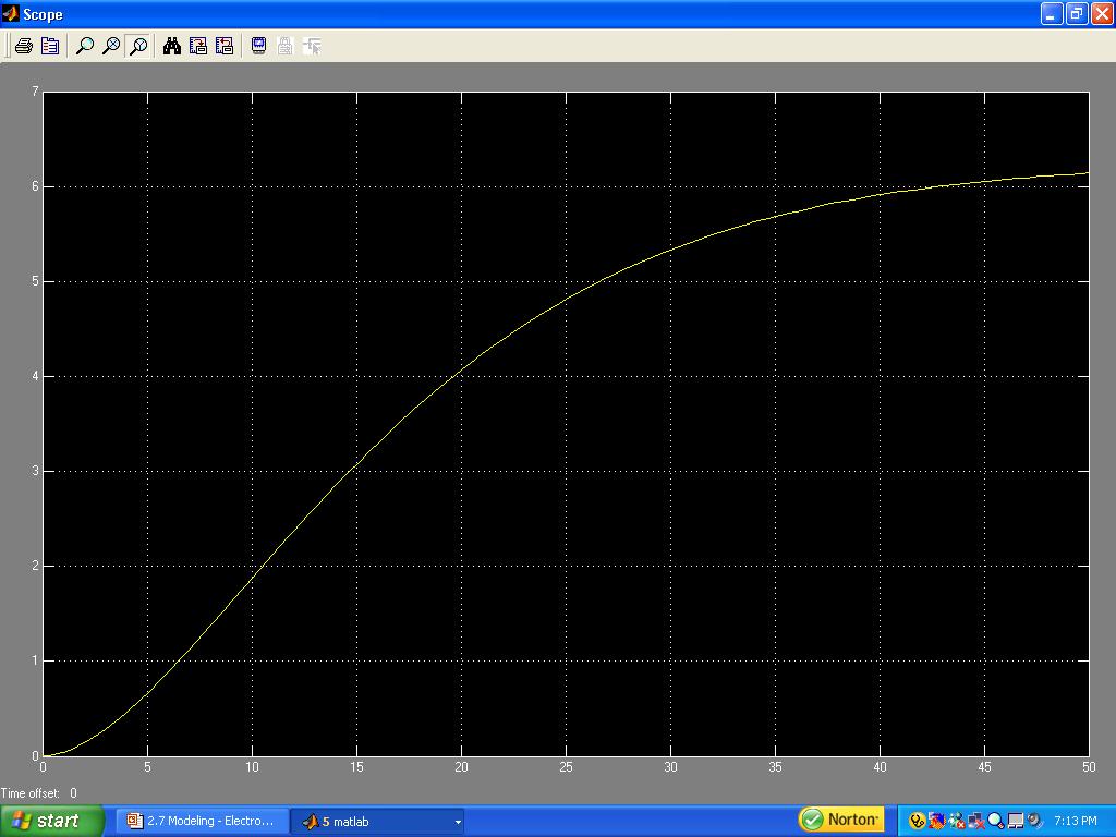
64 Hydraulic Example: Simulation Input, q in, is a step Output, q 2, is taken to a virtual scope Here, we assume all the Cross sectional areas and the resistances equals 1

65 Hydraulic Example: Simulation

66 Another Form of Analogies Potential and Flow Variables When systems are in motion, the energy can be Increased by an energy-producing source outside the system Redistributed between components within the system Decreased by energy loss through components out of the system. Therefore, a coupled system becomes synonymous with energy transfer between systems. Potential Variable = PV Flow Variable = FV

67 Analogies: FV and PV Flow Variable (FV) Potential Variable (PV) Electrical Current Voltage Mechanical Transitional Force Velocity Mechanical Rotational Torque Angular Velocity Hydraulic Volumetric Flow Rate Pressure Pneumatic Mass Flow Rate Pressure Thermal Heat Flow Rate Temperature

68 Which Analogies to use? Force-Voltage makes more physical sense Graphical Representation: Bond Graphs Force-Current makes mathematical sense Sum of Currents= Zero and Sum of Forces = Zero Graphical Representation: Linear Graphs

69 Conclusion Mathematical Modeling of physical systems is an essential step in the design process Simulation should follow the modeling in order to investigate the system response Mechatronic systems involve different disciplines and therefore an appropriate modeling technique to use is block diagrams Analogies among disciplines can be used to simplify the understanding of different dynamic behaviors Dr. Tarek A. Tutunji