Downstream development of a detrital cooling-age signal: Insights from 40 Ar/ 39 Ar. muscovite thermochronology in the Nepalese Himalaya. I.D.

Transcription

1 Downstream development of a detrital cooling-age signal: Insights from 40 Ar/ 39 Ar muscovite thermochronology in the Nepalese Himalaya. I.D. Brewer Department of Geosciences, Pennsylvania State University, University Park, PA D.W. Burbank Department of Geological Sciences, University of California, Santa Barbara, CA K.V. Hodges Department of Earth, Atmospheric, and Planetary Sciences, Massachusetts Institute of Technology, Cambridge, MA Abstract The character and distribution of cooling-ages in modern river sediment provide useful constraints on rates and patterns of uplift and erosion within actively deforming mountain ranges. Such sediment effectively samples all locations within the catchment area, irrespective of remoteness. We evaluate how successfully detrital cooling ages constrain hinterland deformation by examining the modern drainage system of the Marsyandi River in central Nepal. Laser fusion 40 Ar/ 39 Ar data for detrital muscovite collected from 12 separate sites illustrates the downstream development of a detrital age signal that is both systematic and representative of the contributing area. Over the 100-to-200-km length scale of the Marsyandi basin, no significant comminution of the muscovite grains occurs. Comparisons of paired samples indicate that, at short spatial (10s of meters) and temporal (100s of years) scales, the detrital cooling-age signal appears to be stable. The distribution of bedrock cooling ages in a sub-catchment and the Page 1; Brewer et al.

2 resulting detrital signal at the basin mouth can be modeled a function of the erosion rate, relief, hypsometry, drainage area, and thermochronometer distribution. Given that independent constraints are available for most of these variables, the detrital age signal should be a robust indication of the spatially averaged erosion rate. In the Marsyandi, our model predicts ~2-fold differences in erosion rates, with the southern topographic front of the Himalaya experiencing the most rapid rates of exhumation, exceeding ~2 mm/yr. Introduction In the absence of reliable temporal controls, rates of erosion, topographic evolution, and deformation during orogenic growth remain poorly defined. Bedrock thermochronology is typically restricted to rocks currently exposed at the surface, where it provides a limited temporal record because high erosion rates in active orogens commonly remove the older record. Conversely, detrital mineral thermochronology can combine the antiquity of the stratigraphic record with the quantitative analysis of thermochronology [Bernet et al., 2001; Carrapa et al., 2003; Cerveny et al., 1988; White et al., 2002].. Because grab samples in a foreland basin can contain millions of grains, each from a different point within the contributing catchment, detrital samples are potent integrators of orogenic data. When extracted from stratigraphic successions, detrital thermochronology provides the potential to document successive changes in the frequency of cooling ages and rates in an orogenic hinterland. Amid current controversy regarding thermal, flux, and topographic steady state in orogens [Whipple, 2001; Willett and Brandon, 2002; Willett et al., 2001], detrital ages serve to define changes in lag times between mineral cooling and deposition: a key indicator of changing erosion rates or thermal state [Bernet et al., 2001; Bullen et al., 2003; Carrapa et al., 2003]. Page 2; Brewer et al.

3 Before detrital thermochronological data can be reliably interpreted, however, the processes controlling the production of the cooling-age signal need to be explored. Because a detrital sample represents an integration across a catchment, it is critical to know how the observed spectrum of detrital ages is influenced by spatial patterns of erosion, variations in lithology, mechanical breakdown of grains during transport, and differences in sediment production and transport processes and rates. Due to practical limitations on the number of grain ages that can be measured, commonly only one sample is analyzed at a given stratigraphic level or at a point on a river system. Hence, the stability of the detrital age signal should also be assessed: does it vary at spatial scales of 10s of meters and 100s of years? Although the widest applicability of detrital age analyses may be to stratigraphic successions, many of the key controls are impossible to define in ancient catchments, e.g., spatial and temporal variations in erosion rate, lithology, source-area boundaries, topographic relief, and geomorphic processes. The hinterland has frequently been eroded away and even where it still exists, the boundaries of the catchment itself are almost always unknown. Consequently, modern catchments provide the best opportunity to explore the multiple variables that influence the detrital-age signal carried by a trunk stream. Armed with such knowledge, interpretations of data from the rock record can be improved. The distribution of bedrock cooling ages in a catchment can be modeled as a function of topographic relief, erosion rate, and the subsequent geothermal gradient [Mancktelow and Grasemann, 1997; Stüwe et al., 1994]. For 40 Ar/ 39 Ar dating of muscovite when the erosion rate is 3 mm/yr [Brewer at al., 2003], the detrital cooling-age signal is determined by the hypsometry (the distribution of area with elevation) of the catchment. These simple models, however, are applicable to drainage basins with spatially uniform erosion rates and homogeneous distributions Page 3; Brewer et al.

4 of the target thermochronometer (in this case, muscovite). In most active orogens, such restrictions would preclude the study of larger, orogenic-scale drainage systems. In this study, we focus on the extensive detrital system of the complete Marsyandi River, a Transhimalayan river in central Nepal. We examine how the cooling-age signals of tributary catchments combine to produce a modern trunk-stream signal. We use 40 Ar/ 39 Ar analysis of individual muscovite grains to examine how the lithology, erosion rate, and hypsometry of individual catchment areas vary, and we investigate how these parameters control the evolution of the trunk stream cooling-age signal from the headwaters to the foreland basin. This allows us to examine how well the cooling-age signal at the basin mouth represents the contributing area upstream, and hence provides a baseline study for the interpretation of stratigraphic studies of detrital ages. Cooling ages of detrital minerals have been used previously to assess provenance and source-area character [e.g. Adams et al., 1998; Garver and Brandon, 1994; Gehrels, 1998], to estimate the age of the enclosing strata [e.g. Bullen et al., 2003; Carrapa et al., 2003; Garver et al., 1999; Najman et al., 2001], and to reconstruct orogenic cooling and erosion histories [e.g. Brandon and Vance, 1992; Copeland and Harrison, 1990; White et al., 2002].. The wide range in closure temperatures for different thermochronometers allows their application to many types of temperature-dependant geological problems. High-temperature thermochronometers are typically used to date the crystallization ages of minerals, while low-temperature thermochronometers are typically used to investigate the late-stage cooling history. Despite the value of the aforementioned studies, their interpretations are commonly weakened by the unknown variability in parameters, such as erosion rate, relief, or lithology, that modulate the detrital signal. [Stock and Montgomery, 1996] suggested that the range of detrital Page 4; Brewer et al.

5 cooling ages produced by a particular basin, in combination with a specified geothermal gradient, allows a theoretical calculation of basin relief. Brewer et al. [2003] investigated how the interactions between geothermal gradient, erosion rate, and relief can be used in conjunction with the basin hypsometry to predict the distribution of detrital cooling ages. Although these studies reinforce the contention that detrital cooling-age data can provide useful tectonic-geomorphologic insights, the scale of such applications, as previously described, needs to be limited to individual drainages contained within zones of uniform erosion rates. Studies of catchments and their detrital signals at the orogenic scale, however, should consider variable erosion rates, topography, and lithology, because a large catchment produces a complex signal representing an integration of detrital grains from multiple tributaries. In this paper, we build on previous work to investigate the parameters controlling the cooling-age signal from an entire orogenic scale basin. Field data from the Marsyandi valley in central Nepal are used to examine the spatial pattern of erosion in the modern Himalaya. Geological Background The Himalaya represent a favorable study area for detrital age dating because this collisional orogen encompasses stark contrasts in tectonic rates, erosion rates, lithology, and depth of erosion. North of the Himalayan topographic axis, the Indus-Tsangpo suture zone marks the surface boundary between lithologic units of Eurasian plate affinity to the north and Indian plate affinity to the south. After the initial collision at ~50 to 54 Ma [Rowley, 1996; Searle et al., 1997], the downgoing Indian plate was imbricated along a series of south-vergent thrust fault systems, and the Himalaya formed as a result of the subsequent crustal thickening. Deformation continues today and GPS data [Wang et al., 2001; Bilham et al., 1997] indicate that ~40% of the Page 5; Brewer et al.

6 current convergence between the Indian and Eurasian plates currently occurs across the Himalaya. Thrust-fault systems mark many of the principal boundaries between tectono-stratigraphic divisions in the Himalaya. The Main Central Thrust (MCT) system juxtaposes high-grade metamorphic rocks and leucogranites of the Greater Himalayan sequence against lower-grade metasedimentary rocks of the Lesser Himalayan zone. Farther south, the Lesser Himalayan zone is separated from the foreland basin of the Himalaya by the Main Boundary Thrust (MBT) system. The most foreland-wards topographic expression of the Indo-Asian collision, the Siwalik Hills, corresponds to the Main Frontal Thrust (MFT) system. The initiation ages of these major thrust systems are progressively younger from north (20 to 23 Ma for the MCT system) to south (Pliocene to Holocene for the MFT system), although ample evidence exists for episodic out-ofsequence thrusting along these and other less significant fault systems in the Himalayan realm over the Miocene-Recent interval [Hodges, 2000]. The surface trace of the MCT system marks the approximate physiographic transition from the Lower to the Higher Himalaya, where a striking increase in mean elevation and relief occurs. As a consequence, much of the steep southern front of the Higher Himalaya, where erosion rates are likely to be more rapid, is developed on the metamorphic and igneous rocks of the Greater Himalaya sequence. A fourth important fault system bounds the top of the Greater Himalayan sequence: the South Tibetan Fault system. Carrying primarily unmetamorphosed, Neoproterozoic-Paleaozoic clastic and carbonate sedimentary rocks of the Tibetan zone in its hanging wall, the South Tibetan Fault system incorporates a variety of structures, but chief among them are low-angle, north-dipping detachments with normal-sense displacement [Burchfiel et al., 1992]. In the study area, the South Tibetan Fault system comprises two splays, Page 6; Brewer et al.

7 the Chame Detachment Fault and Machapuchhare Detachment Fault, which are separated by the greenschist-to-amphibolite grade marble of the Annapurna Yellow Formation [Coleman, 1996; Hodges et al., 1996]. The Marsyandi River system of central Nepal (Fig. 1) has its headwaters north of the trace of the South Tibetan Fault system and drains portions of the Tibetan, Greater Himalayan, and Lesser Himalayan zones over an area of ~4760 km 2. Its major tributaries flow over subsets of these tectono-stratigraphic zones, and sediment in these tributaries thus samples different zones of bedrock in different proportions. As they flow into the main Marsyandi trunk stream, individual tributary signals are progressively mixed downstream. The Khansar Khola ("khola" is the Nepali word for river) and Nar Khola predominately drain Tibetan zone sedimentary bedrock. The Dudh Khola drains Tibetan zone rocks as well as a major Miocene leucogranite, the Manaslu pluton [Le Fort, 1981]. The Dona Khola flows over exposures of this pluton, as well as a variety of metamorphic rocks of the Greater Himalayan sequence. The Miyardi, and Nyadi rivers have headwaters in the Greater Himalayan zone and exclusively sample this bedrock before emptying into the Marsyandi. The Khudi, Dordi, Chepe, and Darondi rivers flow across the MCT system and thus have sediments with provenances in both the Greater Himalayan and Lesser Himalayan sequences. Methodology Sampling strategy Detritus shed from an evolving mountain belt is primarily transported to the foreland basin by fluvial systems. Along its route, the detrital age signal is influenced by the flux and composition of sediment contributed from tributaries. To create reliable interpretations of modern foreland cooling-age signals, we need to understand the present distribution of cooling Page 7; Brewer et al.

8 ages within the hinterland and how these are eroded and transported downstream. The sampling strategy in this investigation was designed to: a) maximize the statistical constraints on contributions by tributary cooling-age signals; and b) investigate the downstream development of the trunk-stream cooling-age signal; while c) using small enough catchment areas to define adequately the spatial variation in cooling ages across the orogenic catchment. With a finite number of laboratory age analyses, trade-offs are unavoidable between obtaining the optimal representation of any single tributary and reliably reconstructing the evolution of the detrital age signal along the course of the entire river. For example, a focus on very small catchments will increase the resolution of spatial variation in bedrock cooling ages, but leaves fewer analyses to constrain the downstream evolution of the trunk stream. Similarly, more analyses on any individual sample will provide a more reliable characterization of the cooling-age signal, but limit the spatial resolution of the study. Detrital sand samples were collected within the Marsyandi catchment from sites ranging from the Tibetan zone to the junction with the Trisuli River in the Lesser Himalayan zone (Fig. 2). At each sample site, large-grained sand was collected from bars within the modern river channel. Care was taken to avoid the influence of small side tributaries and fill deposits, such as terraces, and to collect samples either upstream of sediment-mixing zones at river junctions or sufficiently below junctions (>1 km) such that sediments could be considered well mixed by these turbulent rivers. Although 27 samples were collected for point counting (to characterize the mineralogical constitution of the sediment), only 14 samples from twelve separate locations were selected for 40 Ar/ 39 Ar dating. Six samples were chosen from the main stem of the Marsyandi River, and five samples were taken at the mouth of major tributaries (Fig. 2). One sample (S-40) represents a Page 8; Brewer et al.

9 sub-catchment within the overall Darondi Khola (S-37), taken to assess the relative input of ages from the Greater Himalayan sequence portion of the basin in comparison to the entire basin. To examine the temporal variability of the detrital signal, two samples were collected from the same location; one from the modern river bed (S-8), and one from a fill terrace elevated 2 m above it (S-9). To examine the natural spatial variability of the detrital signal, samples were collected 45 m apart on the downstream (S-53) and upstream (S-52) ends of the same sandbar. 40 Ar/ 39 Ar Analytical Protocols This investigation focused on detrital muscovite, which has been widely used in detrital mineral geochronology and appears to have fewer problems with excess argon than biotite [Roddick et al., 1980]. Individual muscovite grains between 500 to 2000 mm were analyzed at the 40 Ar/ 39 Ar laser microprobe facility at the Massachusetts Institute of Technology [Hodges, 1998]. This coarse grain size was used because, despite rapid Himalayan erosion, it commonly yields grains with sufficient radiogenic 40 Ar for reliable analysis. Hodges and Bowring [1995] provide additional details on the analytical techniques. Apparent ages calculated for each muscovite with an estimated 2-s uncertainty, obtained by propagating all analytical uncertainties, are available in the data repository. Detrital cooling-age signals are commonly represented as a probability density function (PDF), which represents the probability of finding a grain of a particular age, as a function of the age [Deino and Potts, 1992]. Assuming that a Gaussian kernel represents the distribution of error [e.g. Bevington and Robinson, 1992], a probability density function can be calculated for each grain, given the age (t c ) and analytical uncertainty (s). For a sample of N grains collected from a specific locality, the PDF of individual grains (n) can be combined: Page 9; Brewer et al.

10 P(t) = n= N Â n=1 ( 1 s(n) 2.p.e -(t-t c (n )) 2 2.s (n) 2 ) (1) By normalizing the area under the resulting curve to unity, a summed PDF is generated that represents the distribution of age probability as a function of all the grains analyzed from the sample. Point Counting Cooling-age signals can be used to examine how a trunk-stream signal changes downstream, as successive tributaries contribute varying age populations (as described below). Point counting provides a complementary approach to investigating the trunk-stream age signal that does not rely on thermochronology and is less expensive. When detrital minerals are used as conservative tracers, the relative abundance of a particular mineral species can serve to define the relative contribution from individual tributaries. Although this technique has much lower resolution than the thermochronological approach, it provides an additional constraint on relative erosion rates. In addition, point counting serves to delineate the relative abundance of the target thermochronometer within the Marsyandi study area. As a basis for comparison with and integration into the analysis of detrital cooling ages, point counting was used to quantify the distribution of muscovite and other components within the mm fraction. Of the grains counted in each sample, quartz, plagioclase, alkali feldspar, and micas were the major constituents counted, with additional minerals grouped together, and rock fragments considered to be an additional species. Crystalline carbonate was considered to be a mineral, whereas granular carbonate was considered a rock fragment. This Page 10; Brewer et al.

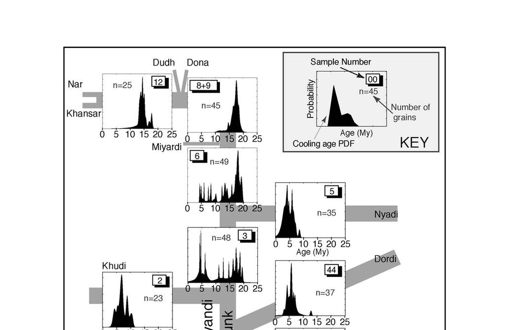
11 method produced an approximate quantification of the major constituents in each sample (Table 1). All reported errors from the point-counting results are taken from the statistical analysis of Van der Plas and Tobi [1965]. To investigate the consistency of individual counts, repeat counts on three samples (S-1, S-2, S-3: Table 1) showed that the results were indistinguishable at the 2- s confidence level. 40 Ar/ 39 Ar results Before attempting to interpret the 40 Ar/ 39 Ar results using a modeling approach, the broad trends in the data illustrate a systematic downstream pattern in the trunk-stream age signal (Fig. 3). The catchment of the sample farthest upstream (S-12) drains the headwaters of the Marsyandi from the edge of the Tibetan Plateau to the crest of the Annapurna massif. The signal is dominated by an age population concentrated between 12 and 16 Ma. One source of these ages may be hydrothermal veins with 40 Ar/ 39 Ar muscovite plateau dates of ~14 Ma that uncommonly occur with the Tibetan zone sedimentary rocks in this area [Coleman and Hodges, 1995]. Alternatively, the catchment contains a small portion of the Annapurna Yellow Formation and the upper Greater Himalayan sequence, which also contribute muscovite. The next sample downstream (S-8/ S-9) was collected to the south of the trace of the South Tibetan Fault System and is influenced by two additional major tributaries, the Dudh and Dona Kholas, which drain the top of the Greater Himalaya sequence and the Manaslu Granite. Whereas the population of ages observed in S-12 is still represented, the cooling-age signal is dominated by a major age population from 15-to-20 Ma. The weak expression of the <15-Ma age population in the downstream sample, and the paucity of muscovite in the upper reaches of the drainage basin suggest that the area upstream of sample S-12 makes a minor volumetric contribution when compared to the additional tributaries found upstream of sample S-8/ S-9. Page 11; Brewer et al.

12 Another 20 km farther downstream, the next trunk-stream sample (S-6) displays the same 15-to-20 Ma population seen in the upstream sample, but contains additional 5-to-15 Ma ages. After the Marsyandi crosses the MCT zone (S-3), the 0-to-10 Ma population becomes more dominant and the 15-to-20 Ma peak represents less than half the total probability. The growing downstream proportion of young cooling ages is clearly influenced by tributaries like Nyadi Khola (S-5), which drains the lower Greater Himalayan sequence and comprises exclusively the 0-to-10 Ma age population. Additional downstream catchments contribute primarily 3-to-14 Ma, such that the lower Marsyandi River (S-52/S-53)shows a dominance of the 5-to-10 Ma age population after the influx of these tributaries. In the Darondi Khola, the sample (S-40) collected above the MCT zone displays a clear 0- to-12 Ma population, whereas sample S-37 at the basin mouth is similar, but includes a single older age component. Prior to merging with the Trisuli River, the trunk-stream Marsyandi sample (S-24) comprises a prominent 5-to-10 Ma signal, a lesser 10-to-15 Ma signal, and a weak 15-to-20 Ma signal. Modeling Although the 40 Ar/ 39 Ar analyses display systematic changes within the Marysandi drainage system, further insights into the hinterland geology, spatial variations in tectonic rates, and interactions within the drainage system could be gained if the distributions of ages were to be translated into the erosion rates via numerical models. Such modeling allows us to examine the impact of individual parameters, e.g., relief, hypsometry, lithology, or erosion rate, and to discriminate between those characteristics of the detrital signal that can be explained by the model, and those that cannot due to the limitations of the initial assumptions. Thus, in combination with the 40 Ar/ 39 Ar data, we use a numerical model to: 1) assess the spatial variation Page 12; Brewer et al.

13 of parameters that control the hinterland cooling-age distributions; 2) understand how these parameters are manifested in the detrital cooling-age signal observed at the basin mouth, and; 3) examine the reliability and resilience of the cooling-age signal. To do this, we construct a theoretical tributary PDF for each basin within the Marsyandi drainage system [Brewer et al., 2003]. These are generated by: 1) inputting the real topographic characteristics of each basin; and then 2) finding the optimal match between the theoretical and observed data PDFs by varying the catchment erosion rate. Once theoretical PDFs have been generated for each tributary, we model the relative contribution from each basin to the trunk stream. Hence, we examine the systematic mixing of age populations in order to understand and predict the downstream evolution of the cooling-age signal within the Marsyandi valley. Modeling the detrital cooling-age signal Initially, theoretical PDFs are generated for each tributary. To predict bedrock cooling ages within a tributary basin, the predicted depth of the closure isotherm at the time when the geochronometer passed through its closure temperature is divided by the rate of erosion. Given a crust of predetermined thermal characteristics, the depth of the closure temperature is a function of the topographic relief and the vertical rate of erosion. For erosion rates 3 mm/yr and topographic relief 6 km, the 350 C closure isotherm of muscovite experiences negligible deflection due to surface topography [Mancktelow and Grasemann, 1997; Stüwe et al., 1994; Brewer et al., 2003]. We use a simplified thermal model [Brewer et al., 2003] to predict the depth of the closure isotherm as a function of the basin relief and a specified erosion rate. The thermal model assumes vertical erosion of material with uniform surface heat flow (57 x 10-3 Wm -2 ) and heat production (1.0 x 10-6 Wm -3 : Fowler, 1990) and conductivity through a steadystate landscape that contains hillslopes at a threshold angle for landsliding (~30 : Burbank et al., Page 13; Brewer et al.

14 1996). These assumptions produce a linear distribution of muscovite cooling ages with elevation. Within a uniformly eroding basin, the cooling-age PDF is controlled by the distribution of area with elevation, i.e., the hypsometry. Thus, the likelihood of sampling a particular age at the mouth of a catchment is a consequence of the fraction of land containing that age. In addition to the thermal assumptions above, the model requires three inputs: relief, hypsometry, and erosion rate. Using this basic model, the larger Marsyandi valley can be broken into individual catchments to represent the area contributing to each of our tributary age samples. By treating each sample separately, we can model changes in the cooling-age distribution due to spatial variations in the erosion rate and topographic relief at the tributary scale. After the topographic relief and hypsometry of each basin are extracted from a 90-m digital elevation model (DEM), the basin erosion rate is the only unknown parameter. Hence, the lowest mismatch [Brewer et al., 2003] between our theoretical PDF and the observed PDF is found by varying the erosion rate within an individual basin. Once the optimal theoretical PDF has been found for a tributary basin, the erosion rate is fixed for any subsequent analysis. Given the theoretical cooling-age distributions from the tributaries, we now need an additional model element to predict how individual basins coalesce to produce the trunk-stream signal. Ultimately, using all the tributaries, we want to predict the whole-basin PDF that serves as a proxy for the modern foreland-basin deposit that would be produced by the Marsyandi River. The relative contribution from an individual tributary is a function of the relative amount of muscovite eroded from the basin per unit time (Fig. 4). For our model, we assume that a long-term steady-state topography exists whereby the regional mean relief, hypsometry, and drainage density are statistically invariant over timescales exceeding 0.1 My. As a consequence of steady-state, the flux of material out of a basin will Page 14; Brewer et al.

15 balance the volume of rock moving into it. With vertical denudation, the eroded volume is the product of the basin area and the erosion rate. The progressive downstream summation of these products should model the evolving trunk stream detrital signal. For flux to be simply proportional to area for a given erosion rate, a uniform distribution of the thermochronologic mineral must be assumed. In the study area, muscovite is expected to be heterogeneously distributed: it is common in high-grade metamorphic rocks, for example, but often absent in carbonates. Hence, the contribution from a carbonate catchment to the detrital muscovite age signal will be negligible, almost irrespective of its erosion rate. We use the percentage of muscovite at the mouth of each tributary, taken from the point counting results (Table 1), to calculate a correction factor for each basin. Note that the percentage of muscovite varies over two orders of magnitude within the Marsyandi river system: any model that ignores a lithological correction factor here will yield profoundly biased results. To model the trunk-stream signal at a particular location, we consider only the predetermined tributary PDFs upstream of the sample. The individual tributary PDFs are combined after correction for lithological variation, erosion rate, and area (Table 2). The resulting PDF curve, with area normalized to unity, represents the theoretical distribution of cooling ages within the trunk-steam sediment at that locality, given the upstream data. To examine the evolution of the detrital age signal, we work systematically downstream by combining the calculated trunk-stream signal upstream of a sample site with the addition from individual tributaries between the two sample sites. In the case where tributary addition is unconstrained by ages at the mouth of a tributary (for example, the inaccessible area represented by the Miyardi Khola: Fig. 2), an erosion rate consistent with the surrounding tributaries, is assigned to the area that minimizes the mismatch of the trunk-stream signal in the sample Page 15; Brewer et al.

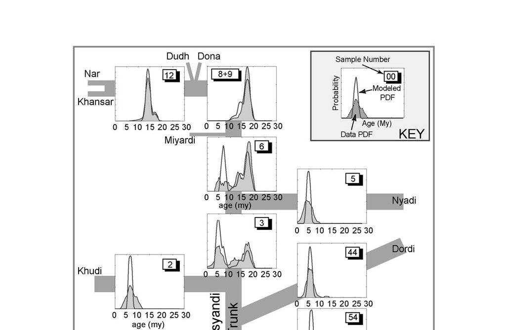
16 directly below the junction. For the purposes of the modeling, the observed and data PDFs are smoothed using a 2-My scrolling window. This reduces the peakedness of the PDFs caused by individual grains, meaning that the calculated mismatch is less affected by individual grain peaks, but instead reflects the overall pattern of the entire signal. PDF modeling results The overall pattern of theoretical PDFs that emerges after combining the results of individual catchments, and then combining them to model the trunk-stream signal, is consistent with the observed data (Fig. 5). The main peaks of the theoretical PDFs generated for each tributary generally align with those of the data PDFs because we minimize the mismatch by varying the erosion rate. In contrast, the tails on either side of the younger peaks are harder to match with our approach (i.e. see the Khudi Khola theoretical PDF for illustration). The trunk stream displays a systematic pattern of change downstream as tributary signals are added. The >15 My peak that is prominent in the upstream samples becomes diluted downstream as the 5-to- 10 My peak becomes increasingly important, although in comparison to the data, the predicted basin mouth PDF (compared to S-24) is relatively depleted in the 10-to-15 My age range. In the upstream reaches of the Marsyandi, a few modifications were made in the modeling in order to find the best match to the observations. Our standard procedure determined the erosion rate that optimized the fit with the observed data for each basin, given its relief and hypsometry, and then used the basin area and abundance of muscovite to predict the basin contribution to the detrital signal of the trunk stream. For our most upstream sample (S-12), draining the Nar and Khansar catchments, the model erosion rate was ~1 mm/yr. Mixing in the modeled contributions from the Dudh and Dona tributaries to the upstream sample (S-12) produced a signal that, in comparison to the next downstream sample (S-8/S-9), was too dominant in the 10-to-15 My age Page 16; Brewer et al.

17 range. In order to reproduce the downstream observations, the relative contribution from the Nar and Khansar had to be reduced by ~50% compared to that indicated by the raw data for the percentage of muscovite (Table 1). The reason for the initial mismatch is unclear, but is likely to reflect two related aspects of the point-counting data. First, grab samples from the Nar/Khansar catchments are characterized by nearly 80% rock fragments (Table 1), most of which are carbonates. This fraction rapidly decreases downstream through a reach with no major tributaries: a behavior suggesting that some combination of dissolution and mechanical breakdown is removing the carbonates from the sand fraction. Second, the muscovite abundances in the upstream areas are low (<1%), but have large errors associated with them. Much of this low abundance in muscovite is attributable to the high frequency of rock fragments, because all other components sum to the fraction not represented by rock fragments. As the rock fragments decrease, the muscovite fraction increases (Table 1). Although this overall trend is clear, the data are noisy at least in part due to the large fractional uncertainties associated with low muscovite abundances. In the context of a mixing model, these rapid changes in relative abundance along a reach with few tributaries makes designation of an appropriate muscovite fraction difficult. Our decision to reduce the upstream contribution by 50% in order to match the observed downstream cooling ages is permissible given both the statistical uncertainties in the abundance data and the rapid, but poorly known, changes in absolute abundance. Although the model results mimic the age distribution from tributaries with older cooling ages, i.e., the upstream catchments, they fail to reproduce the full range of ages in tributaries that yield younger cooling ages. The strong asymmetry observed in the older age tails, in particular, is difficult to replicate (the 8-to-13 Ma ages observed in the Chepe, for example: Fig. 5). Page 17; Brewer et al.

18 Although we assume that each basin is uniformly eroding, in reality, variations in erosion rate in the basins to the south of the range crest are probable because rock-uplift and erosion rates are locally controlled by the geometry of the active subsurface structure [e.g. Lavé and Avouac, 2001; Pandey et al., 1995; Seeber and Gornitz, 1983]. In the absence of detailed sub-tributary data or bedrock ages from these regions, however, we have limited the modeling to the same resolution as our data. The under-represented tails of the observed data certainly account for some of the mismatch seen at the basin mouth (S-24). Another source of mismatch would be areas not included in the modeling (stippled in Fig. 9), yet contributing to the detrital cooling-age signal seen in sample 24. There were insufficient geochronological data from these areas to constrain their erosion rate. Most of these areas lie in the Lesser Himalaya, and if they have intermediate erosion rates, as their low relief and topography would suggest, then they may be an additional source of 10 to 15 Ma ages not represented in the model. Discussion Resilience of the detrital signal. A key concern with the application of detrital dating is the survivability of the thermochronometer in the sediment routing system. If the river network causes a rapid comminution of grains, any sample will only represent a small upstream contributing area that is dependent on the rate of attrition. Such comminution will strongly impact the cooling-age signal that reaches the foreland as information is progressively lost downstream. In the best scenario, an ideal thermochronometer is neither destroyed nor altered during the weathering and transportation history of the sediment. Similarly, post-depositional weathering and diagenesis should not affect the thermochronometer in the resulting sedimentary rock. Page 18; Brewer et al.

19 Both chemical and physical processes may cause the break down of minerals. Previous studies of Himalayan foreland strata with Oligocene to earliest Miocene depositional ages [Najman et al., 1997] that the effects of chemical weathering on muscovite were negligible. Because these sediments are from the same depositional basin and much older than the modern grains we use, and because the Himalaya continues to undergo rapid erosion rates today, we assume that chemical alteration of muscovite does not significantly affect our results.. The process of physical attrition of muscovite grains during their passage through the fluvial system is more difficult to assess. With a hardness of 1 to 2 on Mohs scale and a well-developed basal cleavage, muscovite is susceptible to physical breakdown. However, muscovites apparently survive transport from the Himalayan front to the distal Bengal Fan, a distance of >2000 km, with little disturbance of their 40 Ar/ 39 Ar systematics [Copeland and Harrison, 1990]. Given that the length scale of the Marsyandi catchment is an order of magnitude smaller, physical breakdown of muscovite is likely to be insignificant. The persistence of the 15-to-20 Ma age signal from the upper Greater Himalaya sequence, through all our trunk-stream samples, lends support to this assumption. Rather than being a result of mechanical breakdown, we interpret the downstream decrease in the 15-to-20 Ma age signal to be an effect of dilution. Our modeling assumes a sediment flux proportional to the erosion rate and basin size, but contains no function for the downstream loss of cooling-age signal with distance. Therefore, if comminution were significant over this length scale, the model would be expected to over-represent the 15-to-20 Ma age fraction, particularly in the lower reaches of the river as muscovite grains are progressively destroyed. Instead, the model shows the opposite effect and points to dilution by detritus from more southerly catchments. Overall, mica probably travels in the turbulent wash load of Himalayan rivers, where it experiences few grain-to-grain impacts and little attrition. Page 19; Brewer et al.

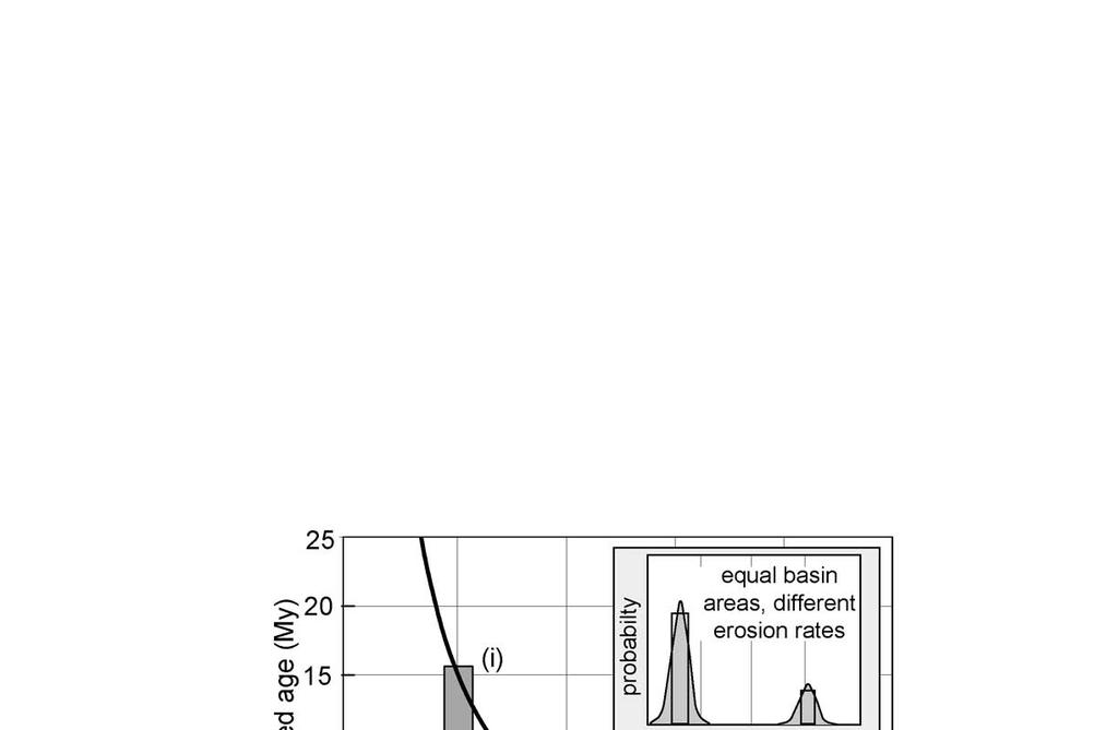
20 Predicted cooling ages are a function of erosion rate and the associated volume of eroded sediment per unit area (Fig.6). Thus, if we wish to investigate the relative proportion of an entire catchment area that is producing a signal of a specific age, we need to correct for the volumetric contribution of that age. For example, although the 15-to-20 Ma age fraction in sample S-24 is relatively minor, because it comprises older cooling ages, it derives from an aerially significant upstream area. Note that the relationship between predicted age and erosion rate (Fig. 6) is not linear in our model because the depth of the closure isotherm varies as a function of denudation rate [Brewer et al., 2003]. Reducing the erosion rate by a factor of two from 2 to 1 mm/yr, for example, has a large effect, changing the predicted cooling age three-fold from 5 to 15 My (Fig. 6). In contrast, the exponential form of this curve means that, when comparing terrains producing cooling ages of >~30 Ma, the difference between the volumetric contribution per unit area as a function of cooling age will be minor. In such cases, the probability distribution of age populations in the sediment will more closely reflect the size of the contributing areas. The reliability of the fluvial signal Two important assumptions in detrital thermochronology studies are: a) the river is efficiently mixing the sediment; and b) the detrital signal is not prone to point sources causing strong temporal variations in the age signal. Landslides, rock falls, and localized storms could influence the latter. If these assumptions are correct, a grab sample should provide a good representation of the entire signal from the river and the upstream catchment. Two pairs of samples were collected to investigate these assumptions. The first pair addressed the homogeneity of fluvial mixing by examining the degree to which samples from different positions at an analogous position on the river yielded comparable age spectra. Sample S-53 and S-52 were collected ~45 m apart on the same modern sand bar in Page 20; Brewer et al.

21 the trunk stream. To test if these two curves are statistically differentiable, we applied the Monte- Carlo methodology to each observed population of ages to generate random grain ages and then summed these ages to generate theoretical PDFs as described by Brewer et al. [2003]. To represent the large range in errors seen in both our single-grain analyses and the summed PDFs (Fig. 3), a more complex method of specifying the 1-s analytical uncertainty was used in this model. Because no consistent relationship of age uncertainty with grain age was observed (Fig. 7a), a PDF was constructed to represent the probability of a specified age uncertainty occurring (Fig. 7b). This error PDF illustrates that, whereas most 1-s analytical uncertainties are <1.5 My, a significant portion of grains has larger associated errors. Therefore, for each modeled grain, the PDF of error ages (Fig. 7b) was randomly sampled (using the same Monte-Carlo methodology), and the resultant 1-s error obtained from that PDF was applied to the model-derived grain age. Based on 500 individual grab samples randomly drawn from the modeled theoretical PDF for S-52/S-53 (Fig. 5), the calculated mismatch between the grab-sample summed PDF and the theoretical PDF [Brewer et al., 2003] was compared against the observed mismatch between S- 52 and S-53. A 2-My smoothing window was used before comparing curves to reduce the influence of individual grains. The theoretical modeling predicted a mismatch of ~20 ± 14% (2s), whereas the observed S-52/S-53 mismatch was 32% (Fig. 8). Hence, the observed mismatch of the two actual samples lies within the expected range of variability, and they can not be proven to be statistically different from each other. Furthermore, in comparison to the observed sample mismatch, the theoretical mismatch is a minimum estimate, because it is drawn from a population defined by the observed samples, whereas the samples themselves were drawn from a broader, but unknown age population. Page 21; Brewer et al.

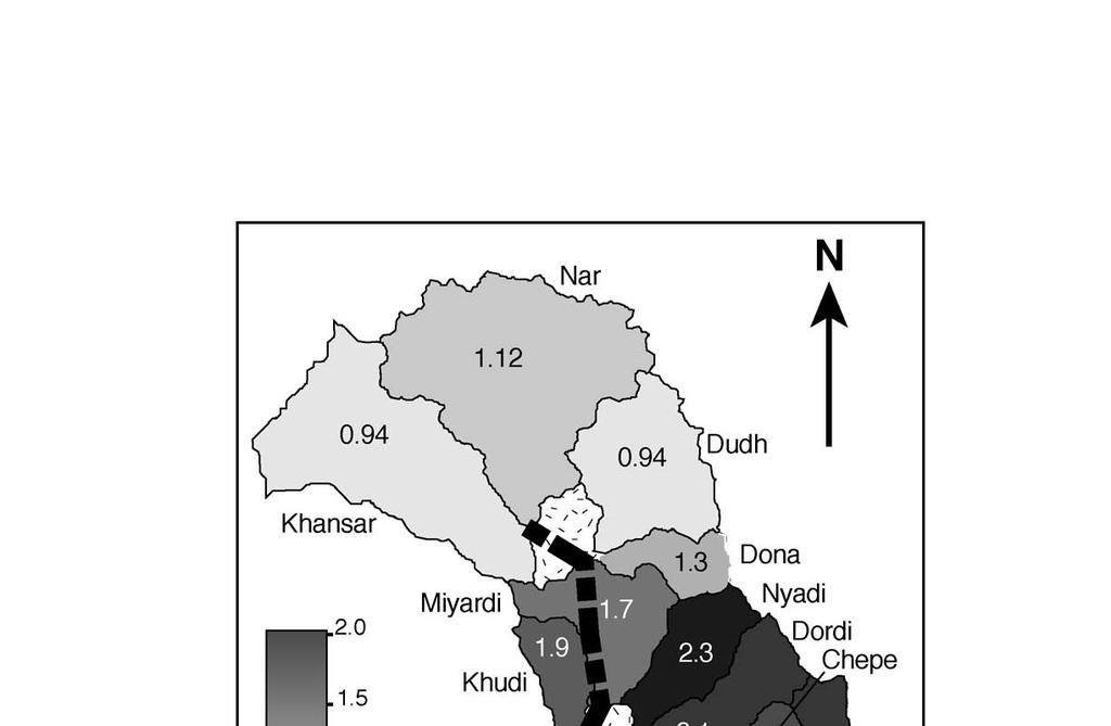
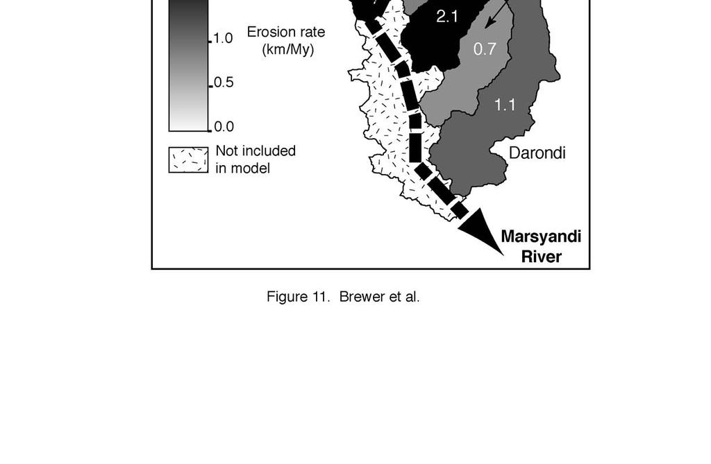
22 The second pair of samples was designed to evaluate the temporal consistency of the detrital cooling-age signal at a particular location. Would samples that are separated by 100 s to 1000 s of years show the same age distribution? If not, the question of sediment storage and production becomes important. Large bedrock landslides would be one scenario where the style of sediment production could affect the detrital cooling-age signal. One can imagine that a landslide might produce a pulse of sediment containing single ages. To test the short-to-medium-term temporal persistence of the detrital signal in one location, a sample (S-08) from the modern riverbed was compared with one (S-09) from an adjacent fill terrace (Fig. 8b) that formed behind a bedrocklandslide dam. The same comparative procedure was applied to these samples, resulting in a 5% mismatch between S-8 and S-9, and an expected mismatch of 21 ± 15% derived from the modeling. Thus the two PDFs are very similar and cannot be considered statistically different. One caveat, however, to this analysis is that the almost unimodal cooling signal may mask temporal variability in sediment supply from the catchment area. Spatial variations of erosion rate Spatial variations in cooling ages derived from low-temperature thermochronology in orogenic belts are commonly used as proxies for analogous variations in erosion rates. The results of the PDF modeling indicate that, within the Marsyandi drainage system, erosion rates vary by over a factor of two: from 0.9 to 2.3 km/my (Fig. 9). The highest rates of 1.9 to 2.3 km/my are found in basins draining the topographic front of the Himalaya. Rates decrease to the north, with the Tibetan Sedimentary Series eroding at rates of 0.9 to 1.1 km/my. Areas to the south of the MCT probably have intermediate rates, but it is difficult to constrain the signal from solely the Lesser Himalaya because most of the rivers also drain the Greater Himalaya sequence. Page 22; Brewer et al.

23 Consider the results from the Darondi Khola (Fig. 3). Approximately 40% of the basin area lies above the MCT zone and is represented by sample S-40. Sample S-37, from the basin mouth, yielded similar ages to sample S-40, but drains the additional area of the Lesser Himalaya, which is 1.5 times the size of the Greater Himalaya portion of the basin. The similarity suggests that either: a) the same erosion rates prevail in throughout the catchment; or b) the Higher Himalaya sequence is producing most of the thermochronometer found at the basin mouth. The latter could be explained either by no effective erosion of the Lesser Himalaya sequence, or low percentages of muscovite in the Lesser Himalayan lithologies. Point counting indicates that the Greater Himalaya sequence is probably dominating the signal because Lesser Himalayan catchments have low abundances of muscovite compared to those draining the Greater Himalayan sequence (Table 1). In addition, lower rates of erosion in the Lesser Himalaya, compared to higher rates on the topographic front, may be an explanation for the older PDF tails that are difficult to fit with the model, for catchments draining both regions. Point-counting results The point-counting results (Table 1) indicate that the sediment composition changes systematically with the downstream addition of tributary material. Samples from the areally extensive Khansar and Nar catchments are rich in rock fragments, containing up to 80%, mainly limestone, clasts from the Tibetan Sedimentary Series. The percentage of rock fragments rapidly decreases downstream, with some addition of granitic rock fragments, to between 20 and 30% towards the basin mouth. The Dudh and Dona Khola, draining the Manaslu granite, are quartzand feldspar-rich and somewhat under-represented in micas. The percentage of muscovite in the tributaries increases rapidly southwards and the Nyadi, Khudi and Dordi all contain 5 to 10% muscovite. The Chepe (S-54) has the largest fraction of muscovite, with over 20% at the basin Page 23; Brewer et al.

24 mouth. Sample S-41 is taken from the Chepe, at the base of the MCT zone, and shows approximately 30% muscovite content. This becomes diluted with the addition of quartz and rock fragments through the lower Himalaya. The two samples in the Darondi show a similar trend of decreasing muscovite and increasing quartz through the lower Himalaya. The percentage of muscovite at the mouth of the Darondi, however, is approximately 5% compared to the much higher value of 23% in the Chepe. Samples are Drainages contained wholly within Lesser Himalayan rocks (S-51, S-56, S-38) all show quartz contents of over 40%, high fractions of rock fragments, and muscovite abundances of 0 to 3%. The rock fragments may be a function of the immaturity of the sediment in relatively small basins (S-38, S-51). As defined by the point counting, the proportion of muscovite in the tributaries is used for the PDF modeling described above. However, the complete mineral proportions of trunk stream and tributaries may also be used for an additional calculation of erosion rate. Mixing the sediment of two rivers together should produce a resulting downstream sample that is representative of the relative contributions from each of the rivers. In reality, the natural variability of the system and point-counting errors mean that the data are more complex. Because of this uncertainty, we use a basic model to examine the general pattern of contributions from each of the inputs and the mixing of the trunk stream. The model uses point-counting data from each of the upstream samples and mixes them to produce a resulting downstream signal. The contribution of each upstream sample is varied from 0 to 100%, and the best solution is picked by finding the minimum residual to the downstream sample. This procedure assumes ideal mixing and no selective deposition, or attrition, of individual mineral species. We have already suggested that the carbonate rock fragments are susceptible to comminution, and hence in some areas they bias the ratios. Therefore, we found Page 24; Brewer et al.

25 that, instead of: a) mixing all the species at once using the method described above; or b) dropping out individual mineral species and recalculating the mixing ratio (with or without renormalizing), the most consistent results were obtained by calculating the mixing ratios for each mineral species individually and taking the mean. This weighted each mineral species equally and eliminated instances where individual mineral species controlled the mixing ratio due to their large volume (e.g. quartz). Based on mixing ratios and catchment areas, relative erosion rates for individual tributaries within the Marsyandi were calculated (Fig. 10). Starting at the most upstream tributary, the sediment volume leaving tributary A was calculated assuming an erosion rate of 1unit per unit area per unit time. For each subsequent downstream tributary, the mixing ratio with respect to the upstream catchment defines a relative volume of contributed sediment that, when divided by tributary area, yields a relative tributary erosion rate. To produce numbers that are of the same order of magnitude as erosion rates calculated by the thermochronology, we normalize the relative erosion rates of a particular basin with the erosion rate derived from thermochronology (in this case using the Dordi Khola). Although there are absolute differences between the erosion rates calculated from thermochronology (Fig. 9) and those calculated from the point-counting analysis (Fig. 11), the general pattern of low erosion in the north of the region, high erosion rates in basins on the southern flank of the main topographic axis, and intermediate erosion rates to the south, is the same. Whereas the PDF modeling suggested variations in erosion rate of up to 2.5 fold, the point-counting model yields variations in predicted rates of >10 fold. These discrepancies are not surprising due to the expected variability of sediment within the river: a) species such as rock fragments will become comminuted downstream; b) carbonate rock fragments and minerals will Page 25; Brewer et al.

26 experience chemical, as well as physical, erosion; and c) hydraulic sorting will be important for minerals with different densities, although sorting appears to have little impact on muscovite in the 500 to 2000 mm size range, as shown by samples S-52 and S-53 (Fig. 8). Conclusions Through examination of the downstream development of a detrital mineral cooling-age signal, this investigation provides insights into long-standing questions concerning the interpretation of detrital-mineral ages. In the past, a sample collected from the foreland basin might be used to interpret erosion rates in the upstream catchment area, but where the erosion was occurring and how much of the basin it represented was unknown. Here, we show that there are systematic and predictable changes in the detrital cooling-age signal of a large, transverse Himalayan river. From the analysis of the Marsyandi Valley detrital system, we learn how the inputs from tributary catchments combine to form the signal at the basin mouth. By implementing a thermalerosional numerical model, we can use the cooling-age distributions from individual tributaries and observable characteristics of the basin (relief and hypsometry) to determine a best-fit erosion rate. The numerical modeling indicates that the detrital cooling-age signal changes systematically in the trunk stream, whereby the input of an age population from an individual tributary is a function of the abundance of the thermochronometer per unit area, the area of the basin, and the rate at which it is eroding. In our analysis, the distribution of muscovite within the catchment is a critical factor in determining the representation of a particular area of the basin in the foreland sample. For example, approximately 30% of the Marsyandi catchment is composed of Tethyan rocks, and yet this represents only a small fraction of the foreland detrital cooling-age signal because of the paucity of muscovite within strata of the Tethyan Sedimentary Series. Page 26; Brewer et al.

27 Comparison of the detrital-age data versus modeling results indicate that comminution of muscovite by fluvial processes seems to be insignificant at the 100 to 200 km scale. The 15-to-20 Ma signal derived from the Marsyandi headwaters is persistent downstream, although decreases in significance. We argue that the calculated volumes of thermochronometer added to the trunk stream are consistent with the downstream dilution of this signal by younger age populations, rather than mechanical breakdown of muscovite. The absence of significant mica loss may be attributable to muscovite moving in the suspended load during the monsoon season, thus encountering less abrasion than during bedload transportation. The variability of the cooling-age signal was tested with samples from 1) different sites on the same sandbar and 2) from nearby deposits of different ages. Our statistical analysis illustrates that although variability exists between samples, the sample pairs were not found to be statistically different at the 95% confidence level: the processes of random selection, from a common parent cooling-age signal, can explain the variation between samples. This indicates that, for at least these two tests, the detrital cooling-age signal is spatially and temporally reliable in this area. The results of the thermochronometry suggest that the topographic front of the Himalaya is eroding faster than the area around it, generating a ~4 to 10 Ma age signal in those basins draining the Greater Himalayan sequence. Areas to the north of the Himalayan topographic axis, on the edge of the Tibetan Plateau, experience the lowest erosion rates and produce grain ages between 10 and 15 Ma for those basins sourced in the Tibetan zone, and 15 to 20 Ma for those basins draining the top of the Greater Himalayan sequence. Intermediate rates are probably found in the lower Himalaya, although the large tributaries draining this zone have headwaters in, and cooling-age signals dominated by, the Higher Himalaya. The pattern of erosion from Page 27; Brewer et al.

28 thermochronology is broadly consistent with the erosion rates calculated from point-counting data. The latter predicts a greater contrast in the erosion rates that should be interpreted cautiously, however, because of the intrinsic variability of sediments within the river system. Two explanations for the overall pattern of the erosion rate are plausible. First, if the MCT and South Tibetan Fault system are active, the high erosion rates of the High Himalaya can be explained by the southwards extrusion of the Greater Himalaya sequence [Beaumont et al., 2001; Hodges et al., 2001]. Alternatively, if the MCT is relatively inactive, then the spatial variation in erosion rate is probably a function of the angle of the underlying Main Himalayan Thrust along which Asia over-thrusts India. Investigations of seismicity indicate the presence of a mid-crustal ramp [Pandey et al., 1995], and increased vertical rock uplift above a steeper section, below the main topographic axis, would account for the spatial pattern of erosion rates [Lavé and Avouac, 2001]. Either of these scenarios introduces the complicating factor of lateral advection. In most investigations to date, cooling ages are converted into rock exhumation rates using an assumption of 1D thermal and kinematic processes. In our model, the depth of the closure isotherm varies as a function of erosion rate and topographic relief, but rock particles still move vertically toward the surface. The thermal structure of an active convergent orogen, however, is not particularly well represented by a simple model of horizontal isotherms, because it is subject to the lateral advection heat energy into the system [e.g. Batt and Braun, 1997; Jamieson and Beaumont, 1988; Jamieson et al., 1998; Willett, 1999]. Rock particles also move laterally, not solely vertically, during erosion and, although beyond the scope of this paper, this complicating factor needs to be considered when assessing the results. This baseline investigation illustrates that, when viewing the array of samples from within the Marsyandi Basin, the downstream evolution of the detrital cooling-age signal in the trunk Page 28; Brewer et al.

29 stream is understandable and can be numerically modeled as a function of contributions from tributaries with variable erosion rates, areas, relief, hypsometries, and muscovite abundances. The interpretation of the most downstream or foreland sample by itself, however, is not necessarily simple because of the complex patterns of tributary mixing. For example, the sample at the basin mouth is dominated by a 4-to-10 Ma population of grain ages, and one might argue that the southern drainages, beginning with the Nyadi catchment (Figs. 2 and 5) and representing ~40% of the area sampled, control the signal. On closer inspection, however, cooling ages from these drainages cannot explain all the intricacies of the older signal: the upstream catchments that drain the upper Greater Himalayan rocks and those of the Tibetan Sedimentary Series, representing ~55% of the basin area sampled, are needed to account for the 15-to-20 Ma age population (Figs. 2 and 5). Our modeling suggests that, despite a larger contributing area, this upstream signal is so much less dominant in the foreland due to the effects of catchment lithology and erosion rate. In this study, we have dated ~500 muscovite grains from 12 locations that have provided new insights into how lithology and drainage-basin characteristics, both easily observable in other modern locations, influence the detrital age signal of the Marsyandi River. Although we argue that the distribution of cooling ages within the foreland provides useful information about the approximate range of erosion rates in the hinterland, considerable caution is needed when interpreting the source and importance of detrital age populations from stratigraphic samples. In order to extract the maximum amount of information from the stratigraphic record, understanding of analogous, but commonly unknown, parameters (hypsometry, catchment boundaries, lithology, erosion rate) that control the modern cooling-age signal is vital. An appreciation both for the complexity of interactions in modern detrital systems and for the Page 29; Brewer et al.

30 primary controls on dominant aspects of the detrital age signal will underpin improved interpretations of the spatial and temporal evolution of orogens based on detrital age studies in the ancient stratigraphic record. Page 30; Brewer et al.

31 References Cited Adams, C.J., M.E. Barley, I.R. Fletcher, and A.L. Pickard, Evidence from U-Pb zircon and 40 Ar/ 39 Ar muscovite detrital mineral ages in metasandstones for movement of the Torlesse suspect terrane around the eastern margin of Gondwanaland, Terra Nova. The European Journal of Geosciences, 10, , Batt, G., and J. Braun, On the thermomechanical evolution of compressional orogens, Geophysical Journal Int, 128, , Beaumont, C., R.A. Jamieson, M.H. Nguyen, and B. Lee, Himalayan tectonics explained by extrusion of a low-viscosity crustal channel coupled to focused surface denudation, Nature, 414, , Bernet, M., M. Zattin, J.I. Garver, M.T. Brandon, and J.A. Vance, Steady-state exhumation of the European Alps, Geology, 29, 35-38, Bevington, P., and K. Robinson, Data reducton and error analysis for the physical sciences, WCB/McGraw-Hill, Bilham, R., K. Larson, J. Freymuller, and P.I. members, GPS measurements of present-day convergence across the Nepal Himalaya, Nature, 386, 61-64, Brandon, M.T., and J.A. Vance, Fission-track ages of detrital zircon grains: implications for the tectonic evolution of the Cenozoic Olympic subduction complex, American Journal of Science, 292, , Brewer, I., D. Burbank, and K. Hodges, Numerical modelling of detrital cooling ages: insights from two contrasting Himalayan drainage basins, Basin Research, 15, , Bullen, M.E., D.W. Burbank, and J.I. Garver, Building the northern Tien Shan: integrated thermal, structural, and topographic constraints, Journal of Geology, 111, , Burchfiel, B.D., C. Zhileng, K.V. Hodges, L. Yuping, L.H. Royden, D. Changrong, and X. Jiene, The South Tibetan detachment system, Himalayan orogen: Extension contemporaneous with and parallel to shortening in a collisional mountain belt, Geological Society of America Special Paper, 269, 1-41, 1992 Burbank, D., J. Leland, E. Fielding, R. Anderson, N. Brozovic, M. Reid, and C. Duncan, Bedrock incision, rock uplift and threshold hillslopes in the northwestern Himalayas, Nature, 379, , Burchfiel, B.C., C. Zhiliang, K.V. Hodges, L. Yuping, L.H. Royden, D. Changrong, and X. Jiene, The South Tibetan Detachment System, Himalayan Orogen: Extension Contemporaneous With and Parallel to Shortening in a Collisional Mountain Belt, 41 pp., Geological Society of America, Denver, Page 31; Brewer et al.

32 Carrapa, B., J. Wijbrans, and G. Bertotti, Episodic exhumation in the Western Alps, Geology, 31, , 2003 Cerveny, P.F., N.D. Naeser, P.K. Zeitler, C.W. Naeser, and N.M. Johnson, History of uplift and relief of the Himalaya during the past 18 Million years: evidence from fission-track ages of detrital zircons from the Siwalik Group, in New Perspectives in Basin Analysis, edited by K.L. Kleinspehn and C. Paola, pp , Springer-Verlag, New York, Coleman, M., and K. Hodges, Evidence for Tibetian Plateau uplift before 14 Myr ago from a new minimum age for E-W extension, Nature, 374, 49-52, Coleman, M.E., The tectonic evolution of the central Himalaya, Marsyandi valley, Nepal, Ph. D. thesis, Massachusetts Institute of Technology, Copeland, P., and M.T. Harrison, Episodic rapid uplift in the Himalaya revealed by 40Ar/39Ar analysis of detrital K-felspar and muscovite, Bengal fan, Geology, 18, , Deino, and Potts, Age-probability spectra for examination of single-crystal 40Ar/39Ar dating results: examples from Olorgesailie, southern Kenya Rift., Quaternary International, 13/14, 47-53, Fowler, C.M.R., The Solid Earth, An Introduction to Geophysics, 490 pp., Cambridge University Press, Cambridge, Garver, J.I., and M.T. Brandon, Fission-track ages of detrital zircons from Cretaceous strata, southern British Columbia: Implications for the Baja BC hypothesis, Tectonics, 13, , Garver, J.I., M.T. Brandon, M. Roden-Tice, and P.J.J. Kamp, Exhumation history of orogenic highlands determined by detrital fission-track thermochronology, Geological Society Special Publication, 154, , Gehrels, G.E., and Kapp, P.A., Detrital zircon geochronology and regional correlation of metasedimentary rocks in the Coast Mountains, southeastern Alaska, Canadian Journal of Earth Sciences, 35, , Hodges, K., and S. Bowring, 40Ar/39Ar thermochronology of isotopically zoned micas: insights from the southwestern USA Proterozoic orogen., Geochemica et Cosmochimica Acta, 59, , Hodges, K., R. Parrish, and M. Searle, Tectonic evolution of the Annapurna Range, Nepalese Himalayas., Tectonics, Hodges, K.V., 40 Ar/ 39 Ar geochronology using the laser microprobe, in Reviews in Economic Geology 7: Applications of Microanalytical Techniques to Understanding Mineralizing Processes, edited by M.A. McKibben and W.C. Shanks, pp , Society of Economic Geologists, Tuscaloosa, AL, Page 32; Brewer et al.

33 Hodges, K.V., Tectonics of the Himalaya and southern Tibet from two perspectives, Geological Society of America Bulletin, 112, , Hodges, K.V., J.M. Hurtado, and K.X. Whipple, Southward extrusion of Tibetan crust and its effect on Himalayan tectonics, Tectonics, 20, , Jamieson, R., and C. Beaumont, Orogeny an metamorphism: a model for deformation and pressure-temperature-time paths with applications to the central and southern Appalachians, Tectonics, 7, 417, Jamieson, R., C. Beaumont, P. Fullsack, and B. Lee, Barrovian regional metamorphism: where's the heat?, Geological Society, London, Special Publications, 138, pp , Lavé, J., and J.P. Avouac, Fluvial incision and tectonic uplift across the Himalaya of Central Nepal, Journal of Geophysical Research, 106, 26,561-26,591, Le Fort, P., Manaslu leucogranite: A collision signature in the Himalaya, a model for its genesis and emplacement., Journal of Geophysical Research, 86, p , Mancktelow, N.S., and B. Grasemann, Time-dependent effects of heat advection and topography on cooling histories during erosion, Tectonophysics, 270, , Najman, Y., M. Pringle, L. Godin, and G. Oliver, Dating of the oldest continental sediments from the Himalayan foreland basin, Nature, 410, , Najman, Y.M.R., M.S. Pringle, M.R.W. Johnson, A.H.F. Robertson, and J.R. Wijbrans, Laser 40 Ar/ 39 Ar dating of single detrital muscovite grains from early foreland-basin sedimentary deposits in India; implications for early Himalayan evolution, Geology (Boulder), 25, , Pandey, M., R. Tandukar, J. Avouac, J. Lave, and J. Massot, Interseismic Strain Accumulation on the Himalayan Crustal Ramp (Nepal), Geophysical Research Letters, 22, , Roddick, J., R. Cliff, and D. Rex, The evolution of excess argon n Alpine biotites - a 40Ar/39Ar analysis, Earth and Planetary Science Letters, 48, , Rowley, D.B., Age of initiation of collision between India and Asia: A review of stratigraphic data., Earth and Planetary Science Letters, 145, 1-13, Searle, M., C. Corfield, B. Stephenson, and J. McCarron, Structure of the North Indian continental margin in the Landakh-Zanskar Himalayas: implications for the timing of obduction of the Spontang ophiolite, India-Asia collision and deformation events in the Himalaya, Geol. Mag., 134, , Seeber, L., and V. Gornitz, River profiles along the Himalayan arc as indicators of active tectonics, Tectonophys., 92, , Page 33; Brewer et al.

34 Stock, J.D., and D.R. Montgomery, Estimating palaeorelief from detrital mineral age ranges., Basin Research, 8, , Stüwe, K., L. White, and R. Brown, The influence of eroding topography on steady-state isotherms. Application to fission track analysis, Earth and Planetary Science Letters, 124, 63-74, Van der Plas, L., and A.C. Tobi, A chart for judging the reliability of point counting results, American Journal of Science, 263, 87-90, Wang, Q., P.-Z. Zhang, J.T. Freymueller, R. Bilham, K.M. Larson, X.a. Lai, X. You, Z. Niu, W. Jianchun, Y. Li, J. Liu, and Z. Yang, Present-Day Crustal Deformation in China Constrained by GlobalPositioning System Measurements, Science, 294, , Whipple, K.X., Fluvial landscape response time; how plausible is steady-state denudation?, American Journal of Science, 301, , White, N.M., M. Pringle, E. Garzanti, M. Bickle, Y. Najman, H. Chapman, and P. Friend, Constraints on the exhumation and erosion of the High Himalayan Slab, NW India, from foreland basin deposits, Earth and Planetary Science Letters, 195, 29-44, Willett, S.D., and M.T. Brandon, On steady states in mountain belts, Geology, 30, , Willett, S.D., Orogeny and orography; the effects of erosion on the structure of mountain belts, Journal of Geophysical Research, B, Solid Earth and Planets, 104, 28,957-28,982, Willett, S.D., R. Slingerland, and N. Hovius, Uplift, shortening, and steady state topography in active mountain belts, American Journal of Science, 301, , Page 34; Brewer et al.

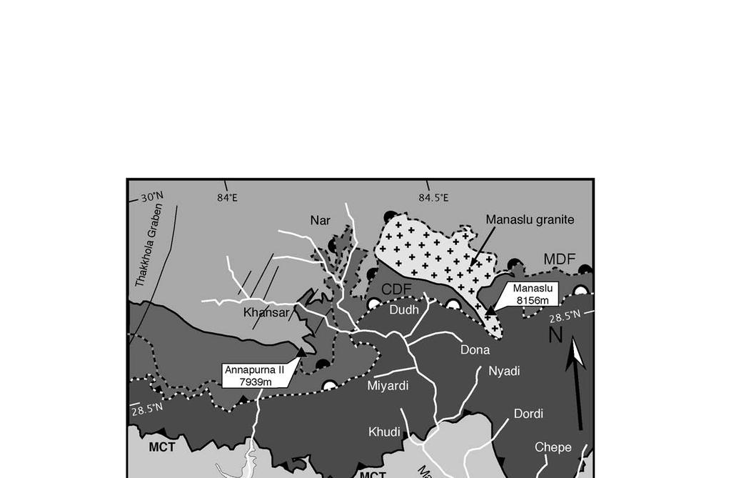
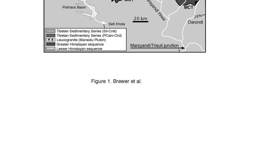
35 Figure captions Figure 1. Simplified geological map of the Marsyandi region adapted from Hodges et al. [1996], initially from Colchen [1996]. The south-verging Main Central Thrust (MCT) separates the Greater Himalaya sequence from the Lesser Himalaya sequence. Other major southverging thrust faults, the Main Boundary Thrust and the Main Frontal Thrust, are to the south of this diagram. The South Tibetan Fault system, with normal displacement, forms two splays in this region: the Chame Detachment Fault (CDF) and the Machhapuchhare Detachment Fault (MDF). Figure 2. Map of Marsyandi drainage system based on a 90-m DEM. Sample locations are displayed with squares (and gray sample numbers) for point-counting sites and circles (and black sample numbers) for 40 Ar/ 39 Ar analysis/point count sites. The Marsyandi drainage (upstream of site 24) is outlined in white. The MCT has triangles indicating south vergence whereas the MDF has half circles indicating extension down to the north. The inset shows the approximate position of the sampling area within Central Asia and the modern geodetic Indo-Asian convergence rate [Wang et al., 2001]. Figure 3. Detrital cooling-age PDFs for samples from the Marsyandi drainage. All axes range from 0 to 25 My on the x-axis and have probability on the y-axis. Areas under the PDF curves (shaded black) represent a total probability of one in each case. The individual plots have been arranged topologically to indicate their position within the Marsyandi River system: geographic locations are shown in figure 2. Additional grain ages in sample 24 (229 ± 18 Ma) and sample 54 (27 ± 0.9 Ma) are not illustrated. Page 35; Brewer et al.

36 Figure 4. Parameters controlling the contribution of an individual tributary to a trunk-stream cooling-age signal. The foreland signal can be modeled as a specified mix of several such tributaries. Figure 5. Model results compared to 40 Ar/ 39 Ar analyses. Real data PDFs (identical to data used in Fig. 3) are shaded gray and smoothed using a 2-My window. Solid black lines are model PDFs generated using the methodology described in the text, and are also smoothed with a 2-My window. The x-axis of each plot ranges from 0 to 30 My, with probability on the y-axis, and the area under each curve represents a probability of one. Figure 6. Predicted cooling ages from our model for specified erosion rates. The non-linearity of the erosion rate-cooling age relation results from changes in the depth of the closure isotherm at different erosion rates. Relative abundances of detrital ages can be predicted based on erosion rates. For two basins of equal area, but eroding at different rates [1 km/my (i) and 3 km/my (ii)], 16-My cooling ages will constitute only 25% of the amalgamated age spectrum (inset). Figure 7. (a) Age versus error (1s) for analyses with greater than 40% radiogenic 40 Ar. No clear relationship between age and error can be seen. Inset (b) shows a PDF generated from the 1s errors. This PDF is smoothed (solid line) and used in the error determination in the numerical model. It can be seen that most assigned errors will be between 0 and 1.5 My. Figure 8. Results of repeat sampling to test: a) the spatial variability of the detrital cooling age signal, and; b) the temporal variation of the signal. For each plot, the shaded PDF is the combined data used in the construction of figure 5, while the PDFs represented by black lines are the contributing data. All curves are smoothed with a 2-My scrolling window. Page 36; Brewer et al.

37 Figure 9. Spatial variation in erosion rates at the drainage-basin scale. Erosion rates are taken from the results of modeling the detrital cooling-age PDFs for individual tributaries. The stippled areas indicate zones not included in the calculations and the dashed gray line indicates the approximate path of the trunk stream. Highest erosion rates are predicted in the middle areas of the Marsyandi Basin, where rivers drain the steep front of the High Himalayas. Slowest erosion rates occur to the north of the topographic axis, in the rain shadow. Figure 10. The procedure used to convert point-counting results into relative erosion rates. Point counting sediment samples from the mouth of drainage A and the mouth of drainage B, in conjunction with a downstream sample AB, can be used to calculate a mixing ratio for the two basins. When combined with basin area, extracted from a DEM, this ratio is used to calculate a relative erosion rate. Figure 11. Spatial variation in erosion rates at the drainage-basin scale based on point-counting data (Table 1) using the methodology illustrated in Figure 10. Relative erosion rates are normalized by the Dordi Khola to allow direct comparison with those derived from the cooling ages (Fig. 9). The stippled areas indicate zones not included in the calculations and the dashed gray line indicates the approximate path of the trunk stream. Note that the overall pattern of erosion is similar to that predicted from cooling ages, with high erosion rates in the middle areas of the Marsyandi Basin and slowest erosion rates to the north of the topographic axis. Page 37; Brewer et al.

38

39

40

41

42

43

44

45 probability a) s-52 smoothed, n=15 s-53 smoothed, n=22 s-52 & s-53 smoothed probability b) s-8 smoothed, n=35 s-9 smoothed, n=10 s-8 & s-9 smoothed Age (My) Figure 8. Brewer et al.

46

47

48