INTEGRATING BASIN MODELING WITH SEISMIC TECHNOLOGY AND ROCK PHYSICS

Transcription

1 INTEGRATING BASIN MODELING WITH SEISMIC TECHNOLOGY AND ROCK PHYSICS A REPORT SUBMITTED TO THE DEPARTMENT OF GOLOGICAL AND ENVIRONMENTAL SCIENCES OF STANFORD UNIVERSITY IN PARTIAL FULFILLMENT OF THE REQUIREMENTS FOR THE DEGREE OF MASTER OF SCIENCE By Wisam AlKawai June 2014

2 Approved for the Department: I certify that I have read this thesis and that, in my opinion, it is fully adequate in scope and quality as a thesis for the degree of Master of Science. Prof. Stephan Graham (Advisor) I certify that I have read this thesis and that, in my opinion, it is fully adequate in scope and quality as a thesis for the degree of Master of Science. Prof.Tapan Mukerji (Co-Advisor) ii

3 Abstract: We explore the link between basin modeling and seismic technology by applying different rock physics models. The data set used in the study is the E-Dragon II data in the Gulf of Mexico. To investigate the impact of different rock physics models on the link between basin modeling and seismic technology, we first model relationships between seismic velocities and porosity and effective stress for well-log data using published rock physics models. Then, 1D basin models at two well locations are built to derive basin modeling predictions of seismic velocities with different rock physics models, and these predictions are compared with average sonic velocities values. Finally, we examine how basin modeling outputs may be used to enhance the inversion process by providing constraints for the background model. For this, we run different scenarios of inverting near angle partial stack seismic data into elastic impedance cube to test the impact of the background model on the inversion results quality. The results of the study suggest that the link between basin modeling and seismic technology is a two-way link in terms of potential applications and the key to refine it is establishing rock physics models that describe changes in seismic signatures with changes in rock properties. iii

4 Acknowledgements: First, I would like to sincerely thank my advisors Prof. Stephan Graham and Prof. Tapan Mukerji for their incredible support and encouragement for completing this work. Without their support and guidance, this work would never have been taken to this level. I look forward to working with both of them for my PhD program. Special thanks to Allegra Hosford Scheirer, Ken Peters and Les Magoon for their valuable support. Thanks to Yunyue (Elita) Li for the helpful discussion about the velocity models in the data. Thanks to Peipei Li for the useful discussion about seismic inversion. I acknowledge the well-log data Copyright (2013) IHS Energy Log Services Inc..I thank Schlumberger/WesternGeco for providing the seismic data. I also thank David Greeley from BP for his great support. Funding and participation in this research is made possible through the support of the Stanford Basin and Petroleum System, Stanford Center for Reservoir Forecasting and Stanford Rock Physics industrial affiliate research programs and through Saudi Aramco Scholarship. Finally, I would like to thank my parents for the great support. iv

5 Contents Abstract... iii Acknowledgements... iv Contents... v List of Tables... vii List of Figures... vii 1. Introduction Motivation Study Area Overview of the Methods Rock Physics Modeling Vp-Vs Modeling Vp-Porosity Modeling Vp-Effective Stress Modeling Basin Modeling D Basin Models Seismic Velocities Calibration Seismic Inversion Near Angle Partial Stack Inversion Inversion Results Basin Modeling Based Background Models Summary Discussion Conclusions Appendices Well-log Data Preparation Interpretation of Vp-Porosity Models Basin Modeling Inputs Basin Modeling Initial Calibration v

6 6.5 Use of Seismic Attributes to Calibrate Basin Models Near Angle Partial Stack Seismic Data Resampling Near Angle Partial Stack Seismic Data Quality Pleistocene Near Angle Elastic Impedance Inversion Miocene Near Angle Elastic Impedance Inversion References vi

7 List of Tables Table 3-1: Basin models stratigraphic intervals input Table 4-1: Inversion scenarios tested in the study Table 6-1: Depths of the top and the base of stratigraphic intervals at wells SS-187 and SS vii

8 List of Figures Figure 1-1: Location of the study area... 3 Figure 1-2: Seismic and well-log data locations... 4 Figure 2-1: Vp-Vs modeling at ST Figure 2-2: Modeling Vp-porosity above 8000 ft... 8 Figure 2-3: Modeling Vp-porosity below 8000 ft... 9 Figure 2-4: Vp normal compaction trends for sandstone and shale Figure 3-1: 1D basin models calibration to porosity and drilling mud weight data Figure 3-2: Default basin modeling outputs of Vp and Vs Figure 3-3: Basin modeling seismic velocities estimates using Vp-porosity models and Vp-Vs model Figure 3-4: Basin modeling seismic velocities estimates using Vp-effective stress relationship combined with Vp-Vs model Figure 4-1: 1D Extracted Pliocene angle dependent wavelet and near angle elastic impedance background models Figure 4-2: Inversion scenarios results Figure 4-3: Near angle elastic impedance background models constrained to basin modeling outputs Figure 4-4: Near angle elastic impedance result using a background model constrained to basin modeling outputs Figure 5-1: Basin modeling default Vp output versus the porosity output Figure 6-1: Estimating the volume of shale (Vshale) at well SS Figure 6-2: Estimating the volume of shale (Vshale) at well SS Figure 6-3: Neutron porosity log clay correction at well SS Figure 6-4: Acoustic impedance changes with porosity and Vshale and acoustic impedance changes vertically along the log Figure 6-5: Operating window of different diagenetic processes in the Plio-Pleistocene sediments (Milliken, 1984) Figure 6-6: Operating window of different diagenetic processes in the Miocene sediments (Gold, 1984) viii

9 Figure 6-7: Cross plot of density and sonic transit time at well SS-187 color-coded by depth zones Figure 6-8: Porosity compaction curves of the lithofacies in the models after calibration Figure 6-9: Porosity-permeability curves of the lithofacies in the models after calibration Figure 6-10: Calibration of the basin model at well SS-187 to elastic properties based on the default velocities outputs in figure Figure 6-11: Calibration of the basin model at well SS-187 to elastic properties based on the velocities outputs in figure Figure 6-12: Original near angle partial stack seismic data with a sampling of 16 ms. 43 Figure 6-13: Extracted wavelet for the Pliocene zone using the original near angle partial stack data combined with well SS Figure 6-14: Pliocene near angle elastic impedance inversion of the original near angle partial stack data Figure 6-15: Resampled near angle partial stack seismic data at 4 ms Figure 6-16: Near angle seismic traces from the original data at well SS-187 for different zones Figure 6-17: Near angle seismic traces from the resampled data at well SS-187 for different zone Figure 6-18: Power spectrums at different zones extracted from the original near angle partial stack seismic data Figure 6-19: Extracted wavelet for the Pleistocene zone Figure 6-20: Near angle elastic impedance inversion at the Pleistocene Figure 6-21: Extracted wavelet for the Miocene zone Figure 6-22: Near angle elastic impedance inversion at the Pleistocene ix

10 Chapter 1: 1. Introduction In this chapter, after describing motivation for this research work, we describe the study area and the dataset used for the work. An overview of the methods used is presented. Subsequent chapters provide the details of the methods and the results Motivation: Basin and Petroleum System Modeling (BPSM) is a powerful technology in hydrocarbon exploration because it allows testing different geologic scenarios with their associated generation, migration and accumulation of oil after modeling deposition and erosion histories and simulating thermal history (Hanstschel and Kauerauf, 2009 and Peters, 2009). BPSM dynamically models changes in rock properties through geologic time by numerically solving coupled partial differential equations with moving boundaries on discretized temporal and spatial grids. This computation results in many outputs of different rock properties including properties such as vitrinite reflectance, temperature, effective stress and porosity. Calibrating geologic scenarios is typically accomplished by comparing basin modeling outputs with existing data. Many calibration data such as vitrinite reflectance (a measure of source rock thermal maturity), temperature and porosity are available just at the borehole vicinity. Seismic attributes such as impedance cubes are spatially extensive. Therefore they offer the potential of a more spatially exhaustive calibration of basin models away from wells by comparing basin model estimates of seismic attributes with observed seismic attributes. However, estimating seismic attributes from 1

11 basin modeling requires combining outputs such as porosity, pore pressure, effective stress and pore fluid saturations with appropriate rock physics models. Extracting seismic attributes such as impedance from seismic impedance inversion requires controls on the low-frequency background trends. Low frequency seismic data below 10 Hz are important in seismic exploration because they experience less attenuation than high frequencies and hence they can penetrate to deeper targets (Dragoset and Gabitzsch, 2007 and Brown, 2010). It is a common practice to control the non-uniqueness of seismic impedance cubes and extend their band-width to include low frequencies when inverting them from band-limited seismic data by combining seismic data with low frequency background models constrained to well-logs and depth trends (Trantola, 1987, Cerney and Bartel, 2007 and Brown, 2010). The fidelity of these background models becomes questionable when well-log data are sparse or even absent. Basin modeling estimates of seismic impedance derived by combining basin modeling outputs with appropriate rock physics models can help to constrain the background models for seismic inversion. Rock physics models are key elements in establishing the link between basin modeling and seismic attributes. This study explores the impact of applying different rock physics models on the link between basin modeling outputs and their associated seismic attributes. It starts by assessing how the basin modeling estimates of seismic velocities change with different rock physics models applied. After that, we explore how the basin modeling outputs can be utilized to constrain background models for seismic impedance. 2

12 1.2. Study Area: The study area is located in the north-central Gulf of Mexico basin off the coast of Louisiana and includes blocks of both Ship Shoal and South Timbalier fields as illustrated in figure 1-1. The Gulf of Mexico basin is a small ocean basin between North American plate and the Yucatan block that formed as a result of an episode of extension and sea-floor spreading during the Mesozoic break up of Pangaea (Galloway, 2008). The structural framework of the basin is dominated by key features like mini-basins and growth faults that resulted mainly from the dynamic interaction between sediments load and salt that was deposited in the Jurassic as a large salt sheet known as Louann Salt. The depositional history of the basin is dominated by fluvial systems and wave dominated deltas and it is characterized by high sedimentation rates during the Cenozoic resulting from formation of the uplands by the Laramide Orogeny (Galloway, 2005). Figure 1-1. Location of the study area. The 3D seismic volume of E-Dragon II data is outlined in red. The Data set used in the study is the E-Dragon II data. It includes 3D seismic data volumes and well-log data as shown in figure 1-2. The 3D seismic data volumes include post stack seismic data, partial angle stack seismic data, velocity cubes for depth conversion and acoustic impedance cube. The well log-data include typical logs such as gamma ray, sonic, bulk density, resistivity and neutron density logs. The data set is supplemented with interpreted horizons for the tops of the Pliocene and the Miocene and biostratigraphic data. 3

13 Figure 1-2. Seismic data location illustrated with a yellow rectangle and locations of avialble well-log data in the study area located in both Ship Shoal and South Timbalier fields within the area of the 3D seismic data volume. Overview of the methods: The study consists of three major parts: a) rock physics modeling, b) basin modeling, and c) seismic impedance inversion. We started the study with rock physics modeling. In this part,we modeled relationships that describe how seismic velocities, Vp and Vs, change with porosity, effective stress and pore pressure. We first modeled the relationship between Vp and Vs for sonic log data at ST-168 that has both P and S waves sonic logs. Then, we modeled Vp-porosity relationships at well SS-187 for the different lithofacies associated with different volume of shale (Vshale) ranges determined because this well has extensive P waves sonic log and neutron porosity log. The details of this modeling are given in the following chapters. Finally, we characterized changes of Vp with effective stress by modeling Vp normal compaction trends with depth for both sandstone and shale at both wells SS-187 and ST-168. The next part of the study is basin modeling at wells SS-187 and SS-160 where we had reasonable age control and calibration data for the basin models. We examined the effect of applying different rock physics models on estimating Vp and Vs from basin modeling results. The goal is to calibrate the basin models to available sonic Vp and Vs data. Following an initial 4

14 calibration step based on porosity and drilling mud weight data, we used three different methods to estimate Vp and Vs from basin modeling results. This gives us an additional calibration and can be used potentially to calibrate basin models away from the wells using Vp and Vs related seismic attributes. It can also be used to calibrate at wells that do not have geochemical calibration data, but have sonic logs available. The last part is angle dependent inversion (ADI) (Anderson and Boggards, 2000 and Jarvis et al., 2004) of near angle partial stack seismic data into near angle elastic impedance. In this part, we first explored the impact of the background model on the inversion results by running different inversion scenarios in which we varied the inversion algorithm as well as the weight assigned to the background model. After running the inversion scenarios, we tested how basin modeling estimates of seismic velocities and density can help to constrain the low-frequency background model for seismic impedance inversion. Chapter 2: 2. Rock Physics Modeling: In this chapter, we present the result of modeling the rock physics modeling which can be divided into three major parts: a) Vp-Vs modeling, b) Vp- porosity modeling and c) Vp-effective stress modeling. Also, we provide some background information about the rock physics modeled we used Vp-Vs Modeling: Modeling Vp-Vs relationship allows predicting Vs changes with different rock properties given the rock physics models describing changes of Vp with these properties. Also, Vs can be 5

15 estimated for wells where only measured Vp sonic logs are available using these Vp-Vs relations. For our study the only well in which both P and S waves sonic logs data were measured is ST-168. Shear waves sonic log data in the other wells were not measured but estimated using Castagna s (1993) Vp-Vs relationship: (km/s) (2-1) that is based on least-squares linear fit to Vp-Vs data of water saturated sandstones.we also examined the mudrock line of Castagna et al. (1985): (km/s) (2-2) We fitted the entire well-log data of Vp and Vs measurements for clean sandstone, shaly sandstone and shale at well ST-168 using these two relationships as shown in figure 2-1. The relationship in equation (2-1) is a fair fit for the clean sandstone data. The shale and the shaly sandstone are generally better fitted with the mudrock line in equation (2-2). These results suggest that the estimated S waves logs in other wells using equation (2-1) are overall an acceptable estimations. In later parts of the study, we volumetrically averaged equations (2-1) and (2-2) when estimating Vs from Vp according to Vshale values. Figure 2-1. Vp-Vs modeling at ST

16 2.2. Vp-Porosity Modeling: We first defined lithofacies based on Vshale. Vshale ranges between 0 and 1 and was defined from gamma ray log values at well SS-187. After defining lithofacies, the Vp-porosity relationships for the sediments above 2438 m were modeled with the constant cement model (Avseth et al., 2001) for all the lithofacies as shown in figure 2-2. This model describes varriations in porosity because of varying sorting for sands that all have a constant cement amount. In this model, we started by modeling the bulk and shear moduli for a dry rock at the critical porosity ø b (which we assumed to be 0.4), using the contact-cement model (Dvorkin et al., 1994) that assumes reduction of initial porosity of a sand pack because of deposition of cement. Then, using the equations for the lower Hashin-Shtrikman bounds we interpolated dryrock bulk ( ) and shear ( moduli for smaller porosities (Avseth et al., 2001): (2-3) and (2-4) where (2-5) and and are respectively bulk and shear modui of the mineral grains that were calculated using a volumetrically weighted Reuss (1929) average of quartz and clay based on the average Vshale value of each lithofacies. Also, we input the coordination number in this model which represent the average number of contacts per grain based on the porosity values using the relationship by Murphy (1982). We assumed a cement fraction of 0.75% quartz cement for sand facies (Vshale < 0.5) and 0.75% clay cement for shale facies (Vshale > 0.5). After obtaining the 7

17 dry-rock bulk and shear moduli values, we calculated the water saturated-rock bulk modulus and shear modulus using Gassmann s (1951) equation. Figure 2-2. Modeling Vp-Porosity above 2438 m. We modeled the deeper part of the well below 2438 m with two different models which are the Han s empirical relation and friable- sand model as shown in figure 2-3. We used Han s (1986) empirical relation for facies with Vshale less than 0.5. This empirical relation is a linear equation based on data of laboratory ultasonic measurements of Vp and porosity for water-saturated sandstones from the Gulf of Mexico at an effective pressure of 40 MPa : (2-6) where is clay volume fraction and is prosoity. For facies with a Vshale higher than 0.5, we used the friable-sand model (Dvorkin and Nur, 1996) that describes Vp-porosity variations with sorting at a specific effective pressure. In this model, we calcualted the elastic moduli values for the critcal porosity of 0.4 end member of a dry rock using Hertz-Mindlin theory (Mindlin, 1949) given the effective pressure and then interpolated the elastic moduli values to lower poroisties using equations (2-2),(2-3) and (2-4). We used in this model a value of MPa for the 8

18 effective stress based on calculating the average effective stress below 8000 ft from the available density log data and drilling mud weight data. The elastic moduli values for the grains of the dry rock were claculated by the same technique used in the constant cement model. After obtaining elastic moduli values for a dry rock, the values of these moduli for a water-saturated rock were calculated again with Gassmann s (1951) equation. Figure 2-3. Vp-porosity modeiling below 2438 m Vp-Effective Stress Modeling: We defined Vp normal compaction trends with depth for sandstone and shale in figure 2-4 to characterize velcoity changes with effective stress and to be able to use these trends in later parts of the study for estimating Vp from stresses values. Defining the Vp normal compaction trends was based on published normal compaction trends for the shallow sediments in the Gulf of Mexico by Dutta et al. (2009): (2-7) for sandstone and (2-8) 9

19 for shale where z is the depth below the mud-line. The trends show an overall good fitting of the sonic Vp data except below a depth of 3658 m for the shale. This can be explained through examining the drilling mud weight data. The well SS-187 drilling mud weight data suggest that the pore pressure is elevated below 3658 m. Also, the higher degree of deviation of the well ST- 168 Vp data for shale from the trend can be explained by an estimating the pore pressure from the drilling mud weight data. When estimating the pore pressure below 3962 m at ST-168, it s even higher than the pore pressure value at SS-187 by about 6 MPa. Figure 2-4. Vp normal compaction trends for sandstone (left) and shale (right). Chapter 3: 3. Basin Modeling: In this chapter, we discuss using seismic velocities to calibrate basin models. We first describe the inputs used to build the basin models as well as the intial calibration of the models. Then, we 10

20 show the results of calibrating basin modeling to seismic velocities after using different rock physics models to drive the basin modeling estimates of seismic velocities D Basin Models: We built 1-D basin models, by defining the ages of the stratigraphic intervals in table 3-1. based on biostraigraphic data combined with interpreted seismic horizons for the top of the Pliocene and the top of the Miocene. Then, we used the average Vshale values in each interval to define the lithology within that interval as a composite lithology of sandstone and shale. Following this, we calibrated the porosity compaction with depth curve of each lithology that was defined by Athy s (1930) law using average porosity values from the corrected netroun porosity log. ( We used a commercial software, Petromod, for the basin modeling). We also used the drilling mud weight data as calibration data for the basin model which can be considered in this case an acceptable proxy of pore pressure because the drilling programs are planned in this basin such that the mudweight is generally increased to prevent fluid flow from formation (Sayers et al., 2002). To match the drilling mud weight data, we perturbed the porosity-permeability curves defiend by multipoint mode (Hanstschel and Kauerauf, 2009) for the lithologies after calibrating the porosity compaction curves until the simulation results showed good calibration to both porosity data and drilling mud weight data as shown in figure 3-1. Stratigraphic Interval Age (Ma) Average Vshale Pleistocene Upper Pliocene Lower Pliocene Upper Miocene Lower Miocene Table 3-1. Basin models stratigraphic intervals input. 11

21 Figure D basin models calibration to porosity and drilling mud weight data Using Seismic Velocities to Calibrate Basin Models: After calibrating the models to porosity and drilling mud weight data, we tested calibrating the models with Vp and Vs data. Using different rock physics models to estimate Vp and Vs can impact this calibration. The first Vp and Vs estimates in figure 3-2 were the default outputs by 12

22 the software without using our calibrated rock physics models. These outputs were obtained after calculating elastic moduli based on the assigned Poisson s ratio for each lithology (Hanstschel and Kauerauf, 2009) and Terzaghi s (1923 and 1943) compressiblity C T that is claculated from the porosity compaction curve using the equation: (3-1) where ø is porosity and is vertical effective stress. The trends of the Vp and Vs outputs seem generally acceptable when compared to the calibration data that represent average sonic velocities values from well logs. However, these outputs always overestimate Vp and Vs resulting in realtively high values compared to the calibraion data. 13

23 Figure 3-2. Default basin modeling outputs of Vp and Vs. The next method we applied to estimate Vp and Vs from basin modeling outputs is combining the basin modeling prosoity outputs with our calibrated Vp-porosity models to obtain Vp. Then, Vs estimates were derived from Vp by simply applying our Vp-Vs relationship. The results of determing Vp and Vs using this method show good calibratin to the average sonic velocities values as illustrated in figure

24 Figure 3-3. Basin modeling seismic velocities estimates using Vp-porosity models and Vp-Vs model. The third method of estimating velocities is based on applying Eaton s (1975) model with an exponent of 3.0: (3-2) where is the overburden pressure, is the pore pressure, is the hydrostatic pressure and is the normal compaction velocity. This method uses the defined normal compaction trends of Vp to calculate Vp from basin modeling outputs of lihostatic, hydrostatic and effecive stresses. The normal compaction trend of Vp at each stratigraphic interval in the model was calcualted through a volumetrically weighted averaging of the normal compaction trends of sandstone and shale according to the average Vshale value in the stratigraphic interval. Similar to the previous method, Vs was estimated from Vp using the Vp-Vs relationship. The results of Vp and Vs estimation using this method show a good match to the calibration data in figure 3-4. However, these results are characterized by less detailed velocity structures when compred to the results from the previous method in figure 3-3. The level of details in the resulting velocities in 15

25 figures 3-3 and 3-4 can be related to the level of details of velocity changes descriped by the rock physics model used to estimate the basin modeling velocity outputs. Figure 3-4. Basin modeling seismic velocities estimates using Vp-effective stress relationship combined with the Vp-Vs model. Chapter 4: 4. Seismic Inversion: This chapter foucses on the sensitivity of the seismic inversion to the background model used to control the inversion result. We first present results of partial angle stack inversion of different 16

26 inversion scenarios designed to test the impact of the background model on the inversion quality. The reason for running partial angle stack inversion is to obtain elastic impedance that is a function of both Vp, Vs and density. Combining the resulting acoustic imedance cube with the available acoustic impedance cube can potentially help any future interpretation work in utlilzing information about Vp, Vs and desnity to classify the lithofacies in the subsurface. Following the inversion scenarios, we show some results of constraining the impedance background model to basin modeling outputs Near Angle Partial Stack Inversion: In this part of the study, we examined the impact of the background model on the quality of inversion results by running six different scenarios of near angle elastic imedance inversion at the Pliocene. In the inversions we varied the inversion algorithm, the weight asisgned to the background model and the qualiy of the backgrouund model used in the inversion process as explained in table 4-1. For all scenarios we extracted an angle dependent wavelet after correlating the near angle partial stack trace with a synthetic seismogram at well SS-187. The synthetic seismogram was created from well-log data using the Zopperitiz (1919) equation for reflectivity for the angle range between 0 to 16. The background model of elastic impedance was conditioned to well-log data using Connolly s (1999) equation for elastic impedance, as described below. The inversion process requires a forward model. Here the seismic traces were modeled by convolving a wavelet with refelctivity series (Tarantola, 1987 and Rusell and Hampson, 1991) : (4-1) The reflectivity series were calculated at every interface across which elastic impedance changes as follow: 17

27 (4-2) The elastic impedance EI was calculated using Connolly s (1999) equation: (4-3) where is density, is the incidence angle and: (4-4) Scenario Algorithm Background Background Model Weight Model I Model-Based Inversion I 0.40 II Model-Based Inversion I 1.00 III Model-Based Inversion I 0.00 IV Sparse-Spike Inversion I 0.40 V Sparse-Spike Inversion I 0.00 VI Spase-Spike Inversion II 0.40 Table 4-1. Inversion scenarios tested in the study. The algorithms used are model-based inversion and sparse spike inverision. (A commercial software, Hampson-Russell CE8\R4.4.1, was used for the inversion). Both of these algorithms start with a low frequency background model and perturb the impedance values in the model until a good match between seismic data and the computed seismic traces is acheived ( Russell and Hampson, 1991). The maximum possible perturbance of the background model is determined by the weight assigned to the background model as part of the input parameters for the inversion. The only major difference between these two algorithms is that sparse-spike inversion assumes sparseness of the reflectivity series (Riel and Berkhout, 1985 and Tarantola, 1987). 18

28 At the start of the inversion process, the angle dependent wavelet (figure 4-1.a) for the Pliocene zone time window was extracted after tying the synthetic seismogram created from well-logs at well SS-187 using the Zoepppritz s (1919) equation with the near angle partial stack trace at the same location. The resulting correlation cofficient achieved after the seismic well-tie is Following the wavelet extraction, background model I was built for the inversion process. Equations (4-3) and (4-4) were used to constrain the background model in figure 4-1.b with the P and S waves sonic logs and the density logs at the wells SS-160 and ST-143. Also, intepreted horizons of the top of the Pliocene and the top of the Miocene were used to constrain the geometry of the model. Using equation (4-3) and (4-4) once again, background model II ( figure 4-1.c) was constrained to the default basin modeling outputs of seismic velocities in figure 3-2 and densities at the locations of wells SS-187 and SS-160. This model has higher values of near angle elastic impedance because of the high values of the default seismic velocities outputs. Having this model allows testing the impact of the quality of the background model on the inversion results. (a) 19

29 (b) (c) Figure 4-1. Extracted Piocene angle dependent wavelet (a), near angle elastic impedance background model I (b) and near angle elastic impedance background model II (c) Inversion Results: The results of the four inversion scenarios are shown in figure 4-2 along with their average cross correlation cofficeints between the modeled synthetic seismic traces and original near angle stack seismic traces. The cofficients were calculated from average cross correlation cofficients for each scenario at multiple locations scattered all over the study area. A comparison between the resulting near angle impedance trace from each inversion scenario at the location of well SS-187 and computed near angle elastic impedance trace from smoothed well-logs at the same well is 20

30 illustrated on the same figure. The results of the inversion scenarios and their associated average cross correlation cofficients vary from each other. The sparse spike scenario results show blocky impedance traces, whereas the model-based scenarios results show ringy impedance traces. This character of the impedance traces from the model-based scenarios is likely to be caused by the quality of the near angle partial stack seismic data. The results of the two scenarios with zero weight assigned to the background model are noisy particularly the sparse-spike that seems even problematic. When comparing the overall quality of the results of the four scenarios, it can be concluded from the results of the inversion scenarios that the sparse-spike scenario IV with a weight of 0.4 assigned to the background model is the best in terms of the quality of the resulting near angle impedance volume. For both algorithms, we see that the background model has a strong influence in constraining the result and it helps to improve the cross-correlation between the modeled synthetic seismic taces and the original seismic traces. It can also be observed that perturbing the background model is necessary to produce an impedance volume with realistic horizontal and vertical variation. Scenario II clearly produced an impedance trace that is very smooth and very close to the near angle elastic impedance values caclualted from the well-log data. However, that scenario resulted in a poor cross correlation cofficient, because it is too smooth and hence it results in a modeled synthetic seismic traces with weak changes of the seismic signatures within the Pliocene. Finally, the results suggest that the quality of the background model is important for obtaining good quality inversion results as can be seen from scenario VI. This background model II used in this inversion scenario has very high elastic impedance values in it and the resulting impedance values are completely off the well-log impedance values. Also, the resulting cross correlation between the modeled synthetic traces and 21

31 the original near angle seismic data is very poor. The results of the inversion scenarios suggest the importance of a background model to control the non-uniqueness of the inversion and the quality of the background model has signficant impact on the quality of the inversion results. Scenario I: average cross correlation coefficient = 0.86 Scenario II: average cross correlation coefficient = 0.37 Scenario III: average cross correlation coefficient =

32 Scenario IV: average cross correlation coefficient = 0.91 Scenario V: average cross correlation coefficient = 0.70 Scenario VI: average cross correlation coefficient = 0.29 Figue 4-2. Inversion scenarios results and comparison of the results with the smoothed calcuated near angle elastic impedance trace at well SS-187 from well-log data. 23

33 4.3. Basin Modeling Based Background Models: Following the inversion results that showed sensitivity to the background model, we tested the idea of using basin modeling outputs to constrain the near angle impedance background model. One motivation for this idea is the work by Petmecky et al. (2009) that showed improvement in the velocity background models for depth conversion after constraining them to basin modeling velocity outputs. Although this idea of using basin modeling outputs to constrain the background model might not be very applicable in this particular case, understanding how basin modeling outputs can constain the background models can have important potential areas where the welllog control is not extensive enough to capture all the changes in seismic velocities due to certain geologic changes. We used the basin modeling Vp and Vs estimates in figures 3-3 and 3-4 since they are close to the calibration data values and we combined them with the basin modeling density output to generate pseudo logs at wells SS-187 and SS-160 obtained after resampling all the combined outputs at a sampling of 0.15 m through linear interpolation. Then, the background models were constrained using the psuedo logs at the wells after calculating near angle elastic impedance from the puedo log data using equations (4-3) and (4-4). We built two different background models based on the different methods for estimating Vp and Vs from the basin modeling outputs. The results are shown in figure 4-3. The background model constrained with the Vp and Vs estimates in figure 3-3 based on Vp-porosity models and the density output is signficantly more detailed than the model constrained with Vp and Vs estimates in figure 3-4 based on Vp-effective stress models along with the density output. Also, the background model constrained with Vp and Vs values based on Vp-porosity relations and density outputs more greatly resembles the background model in figure 4-1.b that was condtioned to well-log data. To further test the idea of using basin modeling outputs to constrain the background models for 24

34 seismic inversion, we ran one more sparse spike inversion scenario using the model in figure 4-3.a with a weight of 0.40 assigned to the background model. The inversion result along with the resulting elastic impedance trace at the location of well SS-187 are illustrated in figure 4-4 with an average cross correlation cofficient between the modeled synthetic seismic and the original near angle seismic data of (a) (b) Figure 4-3. Near angle elastic impedance background models based on : basin modeling density output and estimated Vp and Vs from Vp-porosity models (a) and basin modeling density output and estimated Vp and Vs from Vp-effective stress relationship (b) 25

35 Average cross correlation coefficient = 0.85 Figure 4-4. Near angle elastic impedance inversion result using the background model in figure 4-3.a and compariosn of the resulting near angle elastic impedance at well SS-187 with smoothed near angle elastic impedance calculated from the well-logs Chapter 5: 5. Summary: This chapter summarizes the results of the study in the discussion. We also provide some explaintations of these results in the discussion and we highlight the key conclusions for this work at the end Discussion: The rock physics modeling results of Vp-porosity relationships suggest that there is a change in the type of trends decribing these relationships above and below 2438 m. The trends of Vppororsity relations above 2438 m are generally flatter than those below 2438 m. These flatter trends are recongized as depositional trends (Avseth et al., 2005) where textural variations produced by sedimentation are the major factors controlling porosity changes. The trends below 2438 m of Vp-porosity relationships are generally steeper and these trends are recognized as diagenetic trends in which diagenetic processes such as mechanical compaction are the major factors of porosity reduction. Overall, the Vp-porosity relationships are complex, and they are 26

36 influenced by any changes of textural properties of the sedimetns such as the degree of consolidation and sorting. On the other hand, the models describing the Vp normal compaction trends for sandstone and shale are overall simplistic trends in which Vp smoothly increases with depth as long as the pore pressure of the sediments is hydrostatic. The variations of the 1D basin models velocity estimates indicate high sensitivity of the basin modeling velocity estimates and hence the velocity calibiration to the rock physics models used. The default velocity ouputs in figure 3-2 overestimate the seismic velocities because of the Terzaghi s compressibility model implemented in determining the elastic moduli values. Terzaghi s compressibility in equation (3-1) assumes that the total change in the induced voluemetric strain in a period of time by changing stress with time is equivalent to the total prosity loss in that same time period. This concept simplifies the fact that the total observed induced voluemetric strain in a porous medium is a combination of volumetric strain of the mineral matrix as well as the pores. This simplification leads to overestimating the increase in velocity as porosity decreases and defining very steep Vp-porosity trends. This is illustrated in figure 5-1 by plotting the basin modeling Vp default output versus porosity output at well SS- 187 and fitting them with a straight and then comparing it with examples of some of the rock physics models of Vp-porosity we defined in a previous chapter. This line is clearly steeper than Han s contour shown in the figure and has a higher Vp intercept. Also, the Vp-porosity models on the same figure vary signficantly from each other and using Terzaghi s compressiblity for the entire well is a crude estimation of the Vp-porosity relationship. The results of estimating Vp and Vs in figure 3-3 using Vp-porosity models show more detailed velocity structures than those figure 3-4 estimated by Vp-effective stress models, and this difference can be alotted to the differences in the level of sophstication of the description of changes in seismic velocities 27

37 provided by each of these models as discussed previously. Also, rock physics models that result in more detailed basin modeling estimates of velocities might be more important when calibratting 2D and 3D basin models with velocities where there are probably more heterogenities inherted in the model that should be addressed carefully. Figure 5-1. Basin modeling default Vp output versus the porosity output linear fitting compared with some of the rock physics models of Vp-porosity. The inversion scenarios show sensitivity to both the used algorithm and the weight assigned to the background model. As discussed previously, the inversion scenarios with a weight of zero assigned to the background model showed noisy results which are likely to be caused by the original quality of the data, as well as the non-uniqueness of the inversion process. An important conclusion to draw from the inversion scenario results is that having a good background impedance model is of essence for controlling non-uniqueness of the seismic inversion and obtaining good quality inversion results. The background models conditioned to basin modeling velocity and density estimates support our proposed idea of using basin modeling outputs combined with the appropriate rock physics models to constrain the impedance background 28

38 model and the inversion results obtained using one of these models are very good. Background models derived from basin modeling outputs are sensitive to the rock physics model used. This prompts careful application of rock physics models to determine seismic velocities from basin modeling outputs to condition impedance background models. In seismic inversion, the level of details of the background model is crucial because an accurate and detailed background model provides a better constraint for the inversion process as can be seen from the inversion scenario in figure 4-4 using the background models conditioned to basin modeling outputs. Therefore, applying rock physics models that yield more detailed descriptions of velocity changes with rock properties becomes necessary when constraining impedance background models with basin modeling outputs while a simplistic rock physics model might be good enough in calibrating 1D basin models with seismic velocities, as illustrated previously in figure 3-4. This practice of applying rock physics models appropriately to condition background models of seismic impedance or seismic velocities with basin modeling outputs can have important potential applications in area where the well-log data do not capture certain changes in velocities due to certain geologic changes, and in that case basin modeling can address these geologic changes and appropriate rock physics modeling then can help predicting the velocity changes. Example of these scenarios is an over-pressured basin where the well-logs do not penetrate the over-pressured rocks as in the study by Petmecky et al. (2009) Conclusions: Based on the results of this study, rock physics is the key to link basin modeling outputs with seismic attributes and this link is a two-way link. For basin modeling, basin models can be calibrated to seismic attributes that are spatially extensive such as elastic impedance. For seismic 29

39 technology, basin modeling outputs can constrain building the background models and low frequency trends for impedance inversion and seismic imaging. The required degree of refinement of the link between basin modeling outputs and seismic attributes depend on the scope of the study in which the link is applied. Refining the link depends on the rock physics model used. Therefore, it is an important practice to establish rock physics models that quantify changes of seismic attributes with rock properties and then apply these models to link basin modeling with seismic attributes. The goal of the study and the available data should be taken into full consideration in this practice. Chapter 6: 6. Appendices: 6.1. Well-Log Data Preparation: Given the well log data set, it was important to interpret lithofacies from the available well-log data at well SS-187 to proceed with rock physics modeling in the well. For this purpose, we used the gamma ray log shown in figure 6-1.a to infer the Vshale after picking a sand line and a shale line. After doing a linear interpolation between these two lines, we obtained a log of Vshale ranging between 0 and 1 as shown in figure 6-1.b. Al the outlier values that are either lower gamma ray than the sand line value or higher gamma ray than the shale line were forced respectively to be a Vshale of 0 or 1. Also, a similar Vshale interpretation was done at well ST- 168 in figure

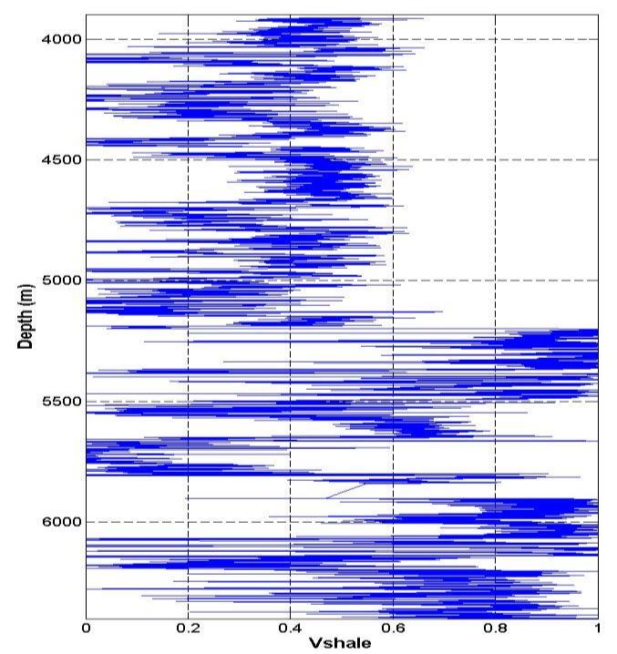
40 Figure 6-1. Estimating the volume of shale (Vshale) at well SS-187 Figure 6-2. Estimating the volume of shale (Vshale) at well ST

41 Another important correction we applied to the log data is correcting the neutron porosity logs for clay minerals. The neutron porosity log tends to overestimate porosity in shale because of the water bounded to the clay minerals in the shale. We assumed in this correction that the porosity of a pure shale is 12% above 1524 m, 10% below 1524 m and above 3048 m and 6% below 3048 m ft. These assumptions of the shale porosity at the depth zones were based on calculating the porosity of a pure shale in these zones based on the bulk density log. The original neutron porosity log is shown in figure 6-3.a along with the corrected neutron porosity log in figure 6-3.b. Figure 6-3. Neutron porosity log clay correction at well SS Interpretation of Vp-Porosity Models: Looking at the modeling results of the Vp-porosity relations, it is important to understand the factors causing the change of the Vp-porosity trends around a depth of 8000 ft (2438 m) as discussed previously to be able to better characterize the basin in any future basin modeling work. To characterize the causes of this change, a cross plot of porosity versus Vshale for well 32

42 SS-187 was generated and color-coded by acoustic impedance (AI) values as in figure 6-4.a. When looking at this plot, two discrete classes can be identified in figure 6-4.b: (1) a class of higher AI values and more rapid changing of AI with porosity given a constant Vshale value and (2) a class with lower AI values and less sensitivity of AI to porosity changes. The first class of higher AI values dominates the lower part of the log below 8000 ft and the second class of lower AI values dominate the upper part of the log above 8000 ft as illustrated in figure 15.c. the transition between the two classes in figure 6-4.c looks very gradual. The depth of the transition of cluster at figure 6-4 is about the same depth of Vp-porosity models trend changes. Therefore, it is very likely that both changes of Vp-porosity trends and changes in the clusters in figure 6-4 are both caused by the same certain changes of the sediments. Understanding these causes requires characterization of the burial and diagenetic histories of the sediments. (a) (c) (b) Figure 6-4. Acoustic impedance changes with porosity and Vshale in (a) and (b) and acoustic impedance changes vertically (c). 33

43 Results from previous works that aimed to characterize the digenetic processes of the sediments across the Gulf of Mexico (Gold, 1984 and Milliken, 1984) show good agreement with the observations of the gradual transition in figure 6-4. These two studies were based on thin sections and x-ray diffraction (XRD) results of samples collected across the Gulf of Mexico for the Pliocene-Pleistocene sediments (Milliken, 1984) and Miocene sediments (Gold, 1984) to identify the different diagenetic processes altering the rocks and come up with a model of how these processes operate. According to these two studies, the processes that cause lithification of the sediments include mechanical compaction, grain alteration and cementation. Grain alteration and cementation processes are thermally driven except for calcite cementation. The models for the depths at which the grain alteration and cementation processes start are shown in figures 6-5 and 6-6. It is clear that a depth of 8000 ft is too shallow to start these processes except for calcite cementation. The observations from both studies suggest that the occurrence of calcite cementation is highly localized and hence it is highly unlikely that calcite cementation produces a volumetric trend with depth. This suggests the likelihood of mechanical compaction being the major factor of the observed changes in trends of the rock physics models of Vp-porosity relationships around 8000 ft. Also, mechanical compaction can explain the gradual transition of AI observed in figure 6-4.c. Another model that supports that concept of mechanical compaction being the leading factor in changing the degree of consolidation of sediments in this shallow part is the paper by Lander and Walderhaug (1999), where they used some samples from the Gulf of Mexico to validate their model of predicting the reservoir quality of the sands. The model they presented suggested that the porosity loss is dominated by mechanical compaction at shallow depths like above 8000 ft before quartz cementation starts to become effective. 34

44 Figure 6-5. Operating window of different diagenetic processes in the Plio-Pleistocene sediments (Milliken, 1984) Figure 6-6. Operating window of different diagenetic processes in the Miocene sediments (Gold, 1984) 35

45 An evidence of that mechanical compaction is the main cause of the change of the rock physics models of Vp-porosity around 8000 ft can be observed when plotting sonic transit time (DT) versus density for shale to interpret the driving mechanism of over-pressure (Bowers, 2002 and Hoesni, 2004). For this reason, we plotted DT versus density for sediments with a Vshale greater than 0.85 in figure 6-7. The sediments clearly follow a compaction line along which DT decreases and density increases and sediments below ft where over-pressure starts deviate from the trend following another parallel line that is above and to the left of original compaction line. This plot suggests mechanical compaction as the main cause of over-pressure around 1200 ft leading to reversal of density and velocity from the normal compaction trends. Therefore, this cross plot shows another evidence of mechanical compaction being the main mechanism altering the rocks in this relatively shallow zone of depth. Figure 6-7. Cross plot of density and sonic transit time at well SS-187 color-coded by depth zones 6.3. Basin Modeling Inputs: When building the 1D basin model, we assigned ages for the top and the bottom of each stratigraphic based on interpreted horizons for the tops of the Pliocene and the Miocene and biostratigraphic data. The depths of the top and the bottom of each stratigraphic interval at well 36

46 SS-187 are specified in table 6-1. For the other model at well SS-160, we used the same stratigraphic intervals of the same ages and lithofacies except that we changed the depth of the top and the bottom of each interval based on biostratigraphic data at the well and interpreted horizons as illustrated in table 6-1. For the boundary condition of the paleo-water depth, we used publications of the paleo-water depth curves in a nearby area in the South Timbalier Field by Stude (1978). The heat flow history was based on a publication by Nagihara and Jones (2005) such that we assumed a constant heat flow through time of 40 mw/m 2. Layer Depth of the Depth of the Depth of the Top Depth of the Top at well SS- Base at well at well SS-160 (m) Base at well SS- 187 (m) SS-187 (m) 160 (m) Pleistocene Upper Pliocene Lower Pliocene Upper Miocene Lower Miocene Table 6-1. Depths of the top and the base of stratigraphic intervals at wells SS-187 and SS Basin Models Initial Calibration: Following building the 1D basin models, the models were calibrated to honor existing porosity and drilling mud weight data. To calibrate to the existing porosity data from the corrected neutron porosity logs, we defined compaction curve of each lithology using Athy s (1930) Law with depth and we used average porosity values from the log to calibrate the compaction curve of each stratigraphic interval as shown in figure 6-8. Following calibrating the porosity compaction 37

47 curve, we started perturbing the permeability and porosity relationship defined by the multipoint model (Hanstschel and Kauerauf, 2009) until a good calibration of the drilling mud weight data is achieved. Peturbing the permeability curves was done based on observations of over-pressure in the drilling mud weight data around which ft which then requires having a seal to generate over-pressure. The resulting permeability porosity curves after calibration are shown in figure

48 Figure 6-8. Porosity compaction curves of the lithofacies in the models after calibration. Red lines represent connection of calibration data points that are user-defined. 39

49 Figure 6-9. Porosity-permeability curves of the lithofacies in the models after calibration. 40

50 6.5. Use of Seismic Attributes to Calibrate Basin Models: After calibrating basin models with seismic velocities, there is a potential of calibrating the basin models with other different seismic attributes that are dependent on seismic velocities such as Vp/Vs Poisson s ratio and Young s modulus. Calibration with these attributes can have potential application such as characterizing a source rock with basin modeling for unconventional plays. Since these attributes are dependent on seismic velocities, having good rock physics models that very well characterize changes of seismic velocities with rock properties is also an essence when calibrating with these attributes. We observed that taking the default velocity outputs by the software to derive Vp/Vs, Poisson s ratio and Young s modulus results in values that are off the average values calculated from well-log data as shown in figure However, we obtained good match between the average calculated values from the well-log data and those derived from the seismic velocities outputs obtained by combining basin modeling porosity output and Vpporosity models as shown in figure Figure Calibration of the basin model at well SS-187 to elastic properties based on the default velocities outputs in figure

51 Figure Calibration of the basin model at well SS-187 to elastic properties based on the velocities outputs in figure Partial Angle Stack Seismic Data Resampling: The original sampling of the partial angle stack seismic data in figure 6-12 is 16 ms. This sampling can be somewhat problematic in the inversion process because of aliasing. An example of a problematic near angle elastic impedance inversion for the Pliocene zone is shown in figure This inversion result was obtained using the same background model I in figure 4-1 combined with an extracted wavelet in figure 6-13 using the well SS-187 along with original near angle stack seismic data with a sampling of 16 ms. The poor quality of the inversion results can be attributed to the aliasing problems in the data used, as well as the extracted wavelet, which both make it difficult to obtain good quality inversion results. To mitigate these difficulties associated with the aliasing of 16 ms sampling, we re-sampled the data in the frequency domain and brought the sampling down to 4 ms as illustrated in figure The resampling was accomplished by first taking the derivative of the seismic data to obtain sparsespike representation of the seismic data and then convolving the spikes with a higher frequency wavelet. 42

52 Figure Original near angle partial stack seismic data with a sampling of 16 ms. Figure Extracted wavelet for the Pliocene zone using the original near angle partial stack data combined with well SS

53 Average cross correlation cofficeint= 0.41 Figure Pliocene near angle elastic impedance inversion of the original near angle partial stack data. Figure Resampled near angle partial stack seismic data at 4 ms. 44

54 6.7. Inversion Quality Control: Looking at the results of the inversion scenarios in the Pliocene zone, the ringy character of the impedance trace resulting from model based inversion is a problematic result that requires further investigation to better understand the limitations in the quality of the inversion outputs. Resampling the data can be a potential source that produces undesired artifacts that limit the quality of the inversion results. To investigate any possible artifacts associated with the resampling of the data, we first plotted the seismic traces of the original near angle stack data at well SS-187 for the Pleistocene, Pliocene and Miocene zones, respectively, in figure Then, we plotted the seismic traces for the same zones at the same location from the re-sampled data in figure Comparing at the seismic traces in figures 6-16 and 6-17, it is clear that the Pliocene zone is characterized by traces of anomalously high frequency that is even much higher than the frequency of the Pleistocene traces. This high anomalous high frequency content of the Pliocene traces is definitely not a signature of the primary signal but rather some anomalous noise or artifact within the data. Figure Near angle seismic traces from the original data at well SS-187 for different zones. 45

55 Figure Near angle seismic traces from the resampled data at well SS-187 for different zones. To further investigate this issue of abnormal high frequency concentrated in the Pliocene Zone, we extracted power spectrums from the original seismic data without any resampling applied for the three zones that are laterally extensive over the area of the seismic data cubes in figure The spectrum of the Pliocene zone shows a dominant frequency of 15.6 Hz, which is slightly higher than the dominant frequency of the Pleistocene which is 15.1 Hz. Although the difference of the dominant frequency is subtle, it suggests an evidence of abnormal high frequency in the Pliocene, because the higher frequency experiences higher attenuation and hence penetrates to shallow depths only. Also, it can be argued from the figure that there is more content of high frequencies around 20 Hz in the Pliocene than in the Pleistocene. On the other hand, the Miocene zone shows a lower dominant frequency of 14.5 H than the other two zones and a lower content of high frequencies around 20 Hz as one can expect from attenuation of high frequencies with depth more rapidly than low frequencies. The key thing to conclude from this analysis is the issue of data quality within the Pliocene zone which can make seismic inversion results in the 46

56 Pliocene zone problematic and limits the quality of the inversion results obtained in the Pliocene zone. Figure Power spectrums at different zones extracted from the original near angle partial stack seismic data. 47

57 6.8. Pleistocene Near Angle Stack Inversion: Following the same method of inversion in the Pliocene zone, we this time inverted the near angle partial stack into elastic impedance within the Pleistocene zone. We used a sparse spike inversion algorithm with a weight of 0.40 assigned to the background model. The background model is model I in figure 4-1. Since the inversion is for the Pleistocene, we extracted a wavelet for the Pleistocene time window in figure 6-19 after accomplishing a seismic well-tie within the Pleistocene zone, given a correlation coefficient of 0.78 at well SS-187 between the synthetic seismic data and the original near angle stack seismic trace within the Pleistocene window. The resulting near angle elastic impedance within the Pleistocene is in figure When examining the quality of the inversion result using the same technique used to examine the inversion results in the Pliocene, we observed an average cross correlation coefficient of 0.93 between the modeled synthetic and the original seismic data. Figure Extracted wavelet for the Pleistocene zone. 48

58 Figure Near angle elastic impedance inversion at the Pleistocene. The red curve is the impedance result at the at location of well SS-187 and the blue curve is the smoothed near angle elastic impedance calculated at the same well Miocene Near Angle Partial Stack Inversion: Similar to the Pleistocene and Pliocene zone, we inverted the near partial angle stack data within the Miocene into near angle elastic impedance using sparse spike inversion with a weight of 0.4 assigned to the background model. We extracted a wavelet specific for the Miocene zone in figure 6-21 after reaching a good seismic well-tie with a correlation coefficient of The resulting near angle elastic impedance for the Miocene is shown in figure The corresponding average cross correlation coefficient with the original near angle stack seismic traces in the Miocene is This better quality of the inversion results of the Pleistocene and the Miocene can be related to the quality of the original near angle partial stack seismic data that showed better quality in the Pleistocene and the Miocene. 49

59 Figure Extracted wavelet for the Miocene zone. Figure Near angle elastic impedance inversion at the Miocene. The red curve is the impedance result at the at location of well SS-187 and the blue curve is the smoothed near angle elastic impedance calculated at the same well. 50