Magnetotelluric measurements for determining the subsurface salinity and porosity structure of Amchitka Island, Alaska

Transcription

1 Appendix 6.A Magnetotelluric measurements for determining the subsurface salinity and porosity structure of Amchitka Island, Alaska Martyn Unsworth, Wolfgang Soyer and Volkan Tuncer Department of Physics and Institute for Geophysical Research University of Alberta, Edmonton, Alberta, T6G 0B9, CANADA Draft Report prepared for CRESP This report by Martyn Unsworth and CRESP 1

2 Summary Amchitka Island, in the Aleutian Islands of Alaska, was used for the underground testing of nuclear weapons from 1965 to Projects Long Shot, Milrow and Cannikin tested warheads with approximate yields of 70, 1000 and 5000 kilotons respectively. Since the test program concluded, there have been concerns about the possible release of radionuclides into the marine environment. The hydrogeology of small islands such as Amchitka is characterized by a layer of freshwater overlying a saltwater layer. The freshwater is derived from rainfall and discharges offshore. The salt water is typically stagnant and a dynamic balance determines the location of the fresh to saltwater interface. The change from fresh to saltwater typically takes place over a broad transition zone. Hydrogeological modeling of this type of groundwater system has provided estimates of the timing and quantities of radionuclides that could be released from the test sites on Amchitka Island. A key parameter in this modeling is the depth of the fresh to salt water transition. However, there is very little data available to constrain hydrogeological models of Amchitka Island. Deep salinity measurements were made in a few boreholes prior to the underground explosions. Remote sensing of subsurface electrical resistivity is a complementary technique for mapping the salinity and porosity of the subsurface. This can be achieved using electromagnetic exploration methods, such as magnetotellurics (MT). The MT method uses naturally occurring radio waves with frequencies Hz to determine the resistivity of the Earth. During the 2004 CRESP Amchitka Island Expedition, magnetotelluric data were collected on profiles that passed through each of the three test sites. After processing and inverting the MT data, two-dimensional models of subsurface electrical resistivity were derived. These showed that a pattern of increasing, decreasing and increasing resistivity was observed at each test site on Amchitka Island. The depth at which resistivity begins to decrease corresponds approximately to the top of the transition zone as the salinity increases. The deeper increase in resistivity approximates the base of the transition zone (TZ), as salinity remains constant and the decreasing porosity causes a rise in resistivity. The following depths were derived from the resistivity models, and uncertainties were estimated in some parameters. Shot depth(m) Salinity at shot (g/l) Top of TZ(m) Top of TZ Possible range(m) Base of TZ(m) Base of TZ Possible range(m) Milrow Long Shot Cannikin The processing was repeated with a range of control parameters, and several independent software packages were used. In each case, the same basic results were obtained. Subject to the limits of the analysis, it appears that each of the underground nuclear explosions was located in the transition zone from fresh to saltwater. This implies shorter transit times to the marine environment than if the shots were located in the saltwater layer. 2

3 1. Introduction 1.1 Background Amchitka Island is located in the western Aleutian Islands of Alaska. From 1965 to 1971 it was used as an underground test site for nuclear weapons that were too large for the Nevada test site. Since the test program was concluded, there have been concerns about the possible transportation of radionuclides into the marine environment. Hydrogeological modeling has constrained the possible transit times and quantities of radiation that could be released into the marine environment. However, there are few constraints on subsurface conditions beneath the island. Prior to the 2004 survey, the depth at which a transition from fresh to salt water occurred was not well known, and this is a key parameter in determining transit times. As part of the CRESP Amchitka Island environmental evaluation in 2004, geophysical data were collected on the island to give additional constraints on subsurface structure. The geophysical work in 2004 focused on electromagnetic imaging that mapped subsurface electrical resistivity. This parameter is sensitive to the porosity and salinity of the groundwater and is thus useful in providing constraints for hydrogeological modeling In this report, the motivation, data collection and analysis are described in detail. The report concludes with an interpretation in terms of models of subsurface salinity and porosity distributions at the Long Shot, Milrow and Cannikin test sites. 1.2 Electrical resistivity and coastal hydrogeology The electrical resistivity of the upper few kilometers of the Earth s upper crust is largely controlled by the presence of interconnected aqueous fluids. The resistivity of a rock formation is a function of four parameters: (1) The salinity of the groundwater (2) The porosity (i.e. the fraction of the rock that is occupied by a fluid) (3) The degree of interconnection of the fluid (i.e. does the fluid form a connected network through the medium, or is it in isolated pockets) (4) The resistivity of the host rock This is illustrated by a set of theoretical calculations in Figure 1. This study represents a typical coastal location, and represents the structure found on Amchitka Island. The salinity values represent a layer of fresh water above the intruding seawater. A transition zone exists with a distributed increase in salinity (Figure 1a). In this example, a relatively high degree of interconnection is assumed, as is typical of fractured near surface rocks. Note that the fluid resistivity (ρ w ) decreases through the transition zone (Figure 1b) as the salinity increases. The first example shows a porosity-depth profile that is constant (Figure 1c). This results in a resistivity profile (ρ o ) that decreases uniformly through the 3

4 transition zone and is then constant at depth (1d). Note that electrical resistivity is the reciprocal of electrical conductivity. Porosity typical decreases with depth (Giles et al, 1998; Rubey and Huppert, 1959) and a more realistic scenario is shown in Figure 1e. This results in an increase in resistivity with depth that opposes the effect of increasing salinity with depth. Note that in the second example (Figure 1f), the transition zone from fresh to salt water is expressed as a decrease of resistivity with increasing depth. The top of the salt water corresponds to the depth at which the bulk resistivity begins to increase again with depth. This is because between depths of 500 and 1200 m in Figure 1f, the resistivity decreases as the groundwater becomes more saline. However, below 1200 m, the salinity is constant at the seawater value and the decreasing porosity causes a rise in resistivity. This theoretical study shows that by remotely sensing the electrical resistivity of the earth, the fluid distribution and composition can be determined from the surface in a noninvasive manner. 1.3 Geophysical techniques for measuring electrical resistivity A number of remote sensing techniques can be used to image subsurface resistivity in the upper few kilometers (McNeill, 1990). Several methods have been used in previous studies in the context of coastal hydrogeology. For studying shallow structure (0-100 m depth) DC (Direct current) resistivity methods can be used to see how far seawater intrudes inland from the shore (Hagemeyer and Stewart, 1990). Inductive loop-loop surveys have also been widely used and have the advantage that direct contact with the Earth is not needed. Ground-based inductive surveys have delineated saline groundwater plumes (Goldstein et al, 1990) and mapped contamination near waste disposal sites (Buselli et al, 1990). For deeper penetration the time-domain method can image to depths in excess of 1 km by using a larger transmitter loop than in the studies listed above (Hoekstra and Blohm, 1990). For imaging at greater depths, the magnetotelluric (MT) technique is most effective. This uses naturally occurring electromagnetic signals in the frequency range ( Hz). MT images subsurface resistivity structure through the skin depth effect, since the depth of signal penetration is inversely related to signal frequency. In audio-frequency magnetotellurics (AMT) frequencies of Hz are used, and if natural signals are not adequate then they can be supplemented by the use of a transmitter in the controlled source audio-magnetotelluric method (CSAMT). This technique was used for characterization at the proposed radioactive waste disposal site at Sellafield in the United Kingdom (Unsworth et al, 2000). The transmitter was necessary to collect data in the presence of extreme cultural noise and this study showed the presence of a saline zone very close to the proposed waste disposal facility. Seawater intrusions can extend a long way inshore. At the Chicxulub impact crater in Mexico, both well logs and MT data show the presence of a freshwater wedge overlying a salt intrusion up to 50 km from the coast (Unsworth et al, 2002). 4

5 Which of these techniques would be most suitable on Amchitka Island? The target depths of 1-2 km are too deep for DC resistivity and are at the depth limit for large loop time domain methods. The logistical effort for large loop time-domain measurements would be significant in the trackless tundra encountered on Amchitka Island. Magnetotellurics (MT) exploration represents the most effective tool for mapping the extent of salt water intrusions beneath the island. 1.4 Magnetotelluric survey design The 2004 MT fieldwork was designed to answer the following questions: (a) Determine the depth of the fresh-salt water interface The hydrogeological modeling of subsurface flow on Amchitka uses observations of subsurface salinity and porosity as inputs (Hassan et al, 2002). However, the available data is quite limited, since very few boreholes were drilled on the island. Possible transit times for radionuclides from the shot cavities to the marine environment are very sensitive to these parameters, and geophysics can constrain these parameters. Based on hydrogeological data available from drilling conducted prior to the underground tests, and other studies of coastal hydrogeology, it was anticipated that a fresh water layer would be present at the surface, with a deep layer of salt water. Prior to the 2004 survey limited data was available to determine the depth of this interface on Amchitka Island. Thus the primary goal of the MT survey was to determine the depth of this interface at each test site and map depth variations across the island. To confirm that an MT survey would be able to address this question, a modeling study was undertaken prior to the fieldwork. A hypothetical resistivity model of Amchitka Island was generated, and this included the approximate bathymetry on each side of the island. The near surface structure was assumed to be layered in the upper few kilometers. Layer 1 represented a typical near surface layer, with significant porosity and saturated with fresh water. Layer 2 had a lower porosity and is also saturated with fresh water. Below this layer 3 is a saltwater layer with lower electrical resistivity. In model A the saltwater was present at 2000 m while in B it is present at 1500 m. Synthetic magnetotelluric (MT) data were computed for these models using the algorithm of Rodi and Mackie (2001) and showed distinct responses. A decrease in apparent resistivity occurs at 11 Hz when the freshwater layer is 1500 m thick. This frequency has decreased to 6 Hz when the layer is at 2000 m depth. The differences between the two apparent resistivity curves are significant, and would be detectable in field MT data with a realistic amount of noise. This study was important in determining the type of MT instrumentation to be used in the survey, since there are two distinct types of MT systems that can be used. Audiomagnetotelluric (AMT) data is specifically designed for shallow exploration and operates in the frequency band 10, Hz. Conventional broadband MT uses 5

6 different magnetic field sensors and collects data from Hz. Using an AMT system would have the advantage of detecting small scale features in the upper few hundred meters of the subsurface. However, it would not be able to detect the decrease in apparent resistivity due to depth variations of the salt water layer. Thus it was decided to use a broadband MT system. Some AMT sensors were taken to Amchitka Island to cover the eventuality that limited high frequency data were required in certain areas. (b) Can subsurface features associated with nuclear testing be imaged with MT? Zones of fracturing, such as the shot cavity and collapse chimney, would be expected to have a lower resistivity, owing to the enhanced porosity. It was expected that such features might be observed, especially for the Cannikin test. Also, a plume of contaminated groundwater might be discernable in the resistivity model as a region of low resistivity. (c) Can faults be detected through their effects on groundwater flow? Hydrogeological models have been used to determine the likely flow patterns and leakage times (Hassan et al, 2002). The predictions made by these models are very sensitive to the presence of faults in the near surface geological section. Faults can act as both seals that prevent groundwater flow or conduits with enhanced porosity and hydraulic conductivity (Caine et al, 1997). The effect of these faults has been detected in a number of MT studies. This includes site characterization at the Sellafield site (Unsworth et al, 2000) and studies of the San Andreas Fault in California (Unsworth et al., 1997). Thus it was anticipated that the Amchitka MT survey might reveal if the hydrogeology is influenced by faults that are adjacent to the underground test sites. 6

7 2. Magnetotelluric data collection on Amchitka Island in 2004 Magnetotelluric (MT) data were collected on Amchitka Island in June 2004 to image the sub-surface resistivity structure. Standard techniques were used for both MT data collection and data processing. The instrumentation used was the V5-2000, a commercial system produced by Phoenix Geophysics in Toronto. MT exploration utilizes recording of both electric and magnetic fields, and thus two distinct types of MT instrumentation were used in the Amchitka Island survey. 5-channel MT sites At these locations both electric field and magnetic field data are recorded. The magnetic fields were measured using induction coils, which are cylinders about 1.5 m long weighing 20 kg. These sites were placed close to roads and tracks to simplify the logistics. 2-channel MT sites (2E) At these stations, only electric fields are measured, and the instrumentation is much lighter. Thus stations more than 500 m from roads used 2E instrumentation. This introduces some error into the data processing sequence, since both electric and magnetic fields are required to compute the apparent resistivity of the Earth with MT. Thus, at 2E sites, the magnetic field from the nearest 5-channel station was used in the data processing. It can be shown that magnetic fields generally exhibit a weaker spatial variation than the electric fields (Mc Neill and Labson, 1987). This assumption is tested in Section 3.1 to assess its validity The 2004 Amchitka Island survey used the two 5-channel MT systems owned by the University of Alberta, two 5-channel systems rented from Phoenix Geophysics and two 2E systems also rented from Phoenix Geophysics. Magnetic fields were recorded with MTC-30 induction coils and electric fields measured with 100 m dipoles using lead-lead chloride electrodes at each end. Prior to the survey on Amchitka Island, all six MT instruments were tested on Adak Island in a disused quarry south of the town site. This testing allowed for calibration of the MT instruments, ensured that all units were working correctly, and allowed new field crew members to be trained prior to the arrival of the expedition on Amchitka Island. It also indicated that wind noise would be an issue in subsequent data collection. Broadband magnetotelluric (MT) data were collected on Amchitka Island at the 29 stations shown in Figures 2 and 3 using the Phoenix V system. Note the distribution of 5-channel and 2E stations. The recording times are summarized in Table 1. Magnetotelluric time series were generally recorded for at least 18 hours at each station, and at a number of locations, MT data were recorded for several days. This field procedure allowed for multiple estimates of the magnetotelluric impedance at each frequency, and permitted the robust processing to separate signal and noise. The instrumentation performed well in the rugged field conditions encountered on Amchitka Island, and no units malfunctioned during the survey. 7

8 3. Magnetotelluric data analysis 3.1 Time series analysis Measurements of the magnetic fields were difficult owing to the strong winds that caused significant ground vibration. This caused the induction coils to move, and the changing component of the Earths static magnetic field along the axis of the coil results in magnetic noise. This type of noise can be removed through use of the remote reference technique (Gamble et al, 1979, Egbert and Booker, 1986), which requires that MT data is simultaneously recorded at two locations. At these locations, it is required that the noise recorded is incoherent, while the MT signal is coherent. On Amchitka Island the strongest noise was in the magnetic fields and due to ground motion caused by wind and wave action. A station separation of a few hundred meters is adequate for effective remote reference processing in this situation, as is illustrated in Figure 4. The MT data that is processed without a remote reference shows artificially low resistivities in the frequency band Hz (Figure 4a). If interpreted directly, these data would suggest the presence of a shallow conductor. When a remote reference station is included in the processing, the apparent resistivity curve becomes smoother and the low resistivities are not observed (Figure 4b). On most days of the survey, all six MT units were recording simultaneously giving an array of MT data. This geometry can be used for multi-station data processing, as described by Egbert (1997), and at some stations gave a modest improvement over the remote reference results (Figure 4c). The arrays used in time-series processing are listed in Table 2. In order to verify that the time-processing scheme of Egbert (1997) had been correctly implemented, an alternative processing code was applied to the MT data for certain sites. This is shown in Figure 5 where the Phoenix Geophysics processing package is compared to the results of Egbert s algorithm for station AM18. Note that the differences are very limited, indicating that the results of the time-series processing can be trusted. Conventional MT data processing assumes that electric and magnetic field data are both recorded at each station. However, at a number of stations on Amchitka Island logistics only permitted the recording of electric fields using the 2E instruments. Thus to process these data, synchronous magnetic fields from an adjacent MT station were used. In general, the spatial variation of magnetic fields is less than electric fields. However, the magnetic fields do vary horizontally and the effect of this phenomena on the resistivity models derived in this report must be considered. Figure 6 shows the effect of using nonlocal magnetic fields in the computation of MT responses at stations AM01 and AM04. While observable differences are observed when a local magnetic field is replaced by a non-local field, the effect is quite small and the main features of the apparent resistivity and phases curves are not altered. Vertical magnetic fields are routinely recorded in MT surveys and can provide good lateral sensitivity to many structures. A vertical magnetometer was installed at each 5- channel station on Amchitka Island. However, it was very difficult to completely bury the vertical induction coils and wind noise was severe on each day of the survey. The remote 8

9 reference technique was applied, but it was not possible to obtain useful vertical magnetic field data. Magnetotelluric data are sometimes affected by static shifts (Jones, 1988). These are the result of small scale, near surface structures that spatially alias the MT data. It was also anticipated that static shifts on Amchitka Island could result from the extreme resistivity contrast associated with the coastline. To address extreme static shifts in MT data, external measurements of near surface resistivity are needed, and time-domain electromagnetic measurements are a common technique. DC (direct-current) resistivity measurements can also be used. In anticipation of severe static shift problems, the University of Alberta DC resistivity system was taken to Amchitka Island. The absence of large static shifts, and limited survey time, resulted in the system not being used. 3.2 Dimensionality of the magnetotelluric data Before MT data can be converted into a resistivity model of the subsurface, it is essential to understand the dimensionality of the data. This determines if a one-dimensional (1-D), two-dimensional (2-D) or three-dimensional (3-D) interpretation must be used. Given the lateral contrast in resistivity produced by the seawater, it is clear that a 1-D approach would not be valid. Thus, it was required to see if a 2-D approach would be applicable. A 2-D analysis is much simpler than a full 3-D analysis, but must be carefully justified. The geoelectric strike direction was computed using the method of Caldwell et al (2004) and the results are summarized in Figure 7. The blue and red lines at each station show the strike direction at each station for three frequency bands. Note that there is a 90 ambiguity in the strike angle. As the frequency decreases, the depth sampled by the MT signals increases. At high frequency ( Hz) the strike direction is poorly defined and the MT data are approximately 1-D (see the MT pseudosections in section 3.3 for additional evidence for this). However at frequencies below 10 Hz, a well defined strike of N55 W or N35 E is observed. External information must be used to determine which of these directions is correct. Since the geometry of the low resistivity seawater dominates the resistivity structure, it is clear that an island parallel strike of N55 W is appropriate (Figure 2). The vertical magnetic fields can also give an idea of dimensionality and strike direction. However, owing to the low quality of these data in the Amchitka Island survey, this was not possible for this dataset. Thus on the basis of the above analysis, the data can be considered 2-D, with a strike (invariant) direction approximately parallel to the axis of the island. The MT data were rotated mathematically to this co-ordinate system for all subsequent analysis. 9

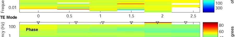
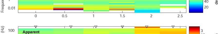
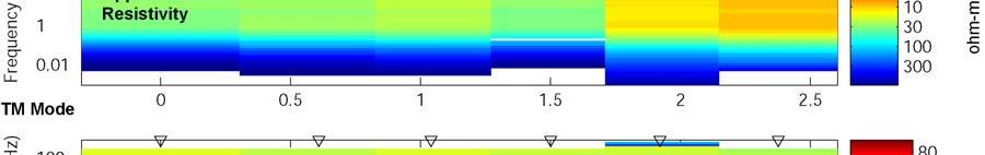
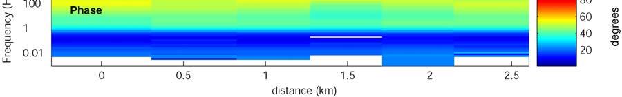
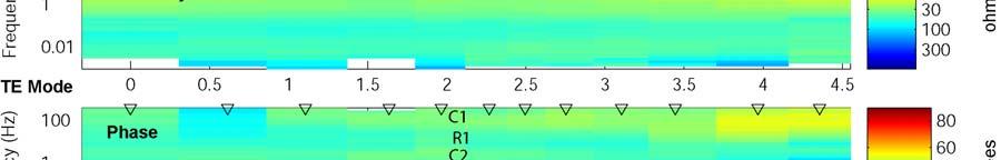
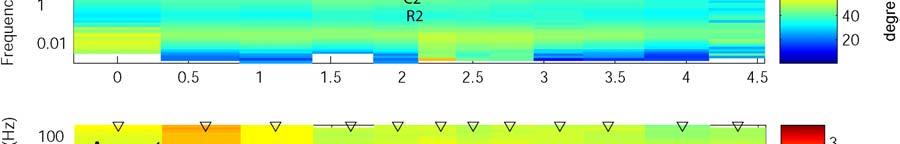
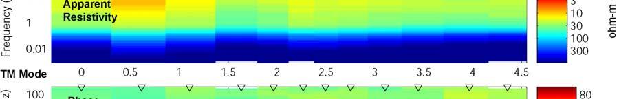
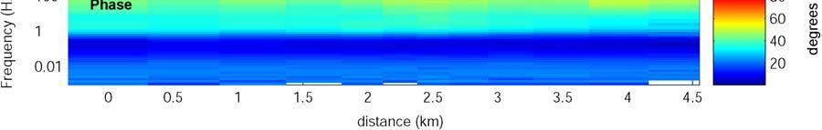
10 3.3 MT pseudosections, apparent resistivity and phase curves Long Shot line A typical apparent resistivity and phase curve for an MT station on the Long Shot profile is shown in Figure 5. The electric currents flowing along the island comprise the transverse electric (TE) mode, while electric current flowing across the island comprise the transverse magnetic (TM). In a 1-D configuration, these two modes will give identical values of apparent resistivity and phase. However, over a 2-D Earth the apparent resistivity values computed from the TE and TM mode will be different. Since the depth of MT signal penetration increases as frequency decreases, the horizontal axis can be considered as a proxy for depth. At high frequency (shallow depth) the apparent resistivity is approximately constant at a value of 30 Ωm. Below a frequency of 1 Hz, the TE and TM curves diverge. The TM mode curve shows high apparent resistivities, while the TE-mode exhibits more modest values. This basic pattern is observed at essentially all MT sites on Amchitka Island (Figure 8), and is due to the socalled ocean effect. This occurs because the low resistivity ocean layer increases the TMmode electric currents that flow across the island. The apparent resistivity is the ratio of electric to magnetic field strengths, and this increases the apparent resistivity. Note that the ocean effect also lowers the phase of the TM mode. Thus to determine the structure in the upper 1-2 km beneath the surface of the island, it is necessary to examine data above a frequency of 0.1 Hz. As frequency is decreased from 300 Hz a subtle oscillation in the TE mode apparent resistivity can be observed. In the frequency band Hz the apparent resistivity is low (i.e. it is conductive). A subtle pattern of resistive (30-10 Hz), conductive (3-0.3 Hz) and resistive ( Hz) features can be seen in the apparent resistivity data at most stations in the centre of the island (Figure 6). The MT phase also exhibits these changes. A phase angle above 45 is considered high and indicates a conductor, while a phase below 45 is considered low and indicates a resistive structure. Note that a pattern of high-low-high-low TE phases can be observed from Hz. These subtle oscillations in apparent resistivity and phase above 0.1 Hz are due to an approximately layered resistivity structure in the upper 1-2 km of the subsurface. The variation in MT data along each profile can also be displayed in pseudosection format. This is a contoured plot of apparent resistivity or phase with distance on the horizontal scale and frequency on the vertical scale. Since lower frequencies penetrate deeper into the Earth, this gives an impression of how resistivity varies with depth. The Long Shot pseudosection is shown in Figure 9 and the pattern of conductive-resistiveconductive-resistive can be seen in both TE mode apparent resistivity and phase (labeled C-R-C-R). Note also that the TM-mode pseudosections show the high resistivity and low phase of the ocean effect below a frequency of 0.1 Hz. This obscures the oscillations due to the layered structure in the upper 1-2 km of the island. Note that the relatively smooth variation in apparent resistivity across the island on each profile indicates a smooth spatial variation in resistivity. 10

11 3.3.2 Milrow line The Milrow line pseudosection is shown in Figure 10, and is similar to that observed on the Long Shot line. The pseudosection shows more evidence of noise than the other profiles, mainly because recording times for this profile were quite short, and less than 6 hours at some stations Cannikin line The Cannikin pseudo section is shown in Figure 11. Note that near surface resistivity values are a little higher than on the Long Shot profile and again the ocean effect dominates the TM data. The conductive-resistive-conductive-resistive pattern can be seen in the TE mode apparent resistivity, but it is not as clear as on the Long Shot profile. However, this pattern is clear in the TE phase, especially to the west of the Cannikin ground-zero. 3.4 Magnetotelluric data modeling and inversion To interpret the MT data, the next step is to take the MT data that is a function of frequency and convert it into a model of subsurface resistivity as a function of true depth. The dimensionality analysis described above showed that a two-dimensional (2-D) approach is appropriate. In this study, extensive 2-D inversions were used and a number of 3-D forward calculations were performed to validate this approach. The 2-D NLCG6 inversion algorithm of Rodi and Mackie (2001) was used in this study. The NLCG6 algorithm uses non-linear conjugate gradients and is a stable algorithm that is widely used by both academic and industrial geophysicists. It has been used a number of previous studies at the University of Alberta, and the use of the algorithm is well understood. The inverse problem of magnetotellurics requires that a finite set of noisy MT data is converted into a resistivity model of the Earth that accounts for the measured MT data. This inverse problem is non-unique (Parker, 1994) and it can be shown that if a solution can be found, then an infinite set of models can also be found. Thus the inversion of MT data requires that additional constraints are applied to the resistivity model to give a unique solution. This process of constraining the solution is termed regularization (Tikhonov and Arsenin, 1979) and generally requires that the model is spatially smooth, and/or close to a starting model. As described above, interpretation of MT data from a coastal environment requires that the low resistivity of the seawater is correctly modeled. This is because the seawater is a stronger conductor than most features present on the surface of the Earth. Thus a first stage in MT data analysis was to generate a 2-D bathymetry model for each profile. This used data courtesy of Mark Johnson at the University of Alaska, Fairbanks. A standard salinity was assumed for both the Bering Sea and Pacific Ocean, which yields a seawater resistivity of 0.3 Ωm. A starting resistivity model was developed with a 100 ohm-m 11

12 seafloor and the simplified bathymetry (Figure 12). Two methods were used to include the conductive ocean in the inversion process. In the first, the seawater resistivity was fixed during the inversion process. This was found to be somewhat unstable and resulted in a spatially rough resistivity model beneath the island. This occurs because any inaccuracy in seawater depth cannot be overcome by extending the seawater conductor to depth. Rather the inversion placed artificial conductors beneath the island. A much more satisfactory approach was too use a softer constraint that simply allowed the regularization to find the smoothest model compared to the starting model. This approach was found to be much more stable Long Shot profile inversions Inversion parameters for the Long Shot inversion model shown in Figure 13 included: Error floor for apparent resistivity 20% Error floor for phase 4% Trade-off parameter, τ = 3; Vertical to horizontal smoothness control parameter, α = 1; Frequency band Hz The inversion automatically estimated the static shift coefficients, but these were small for this profile (see discussion above about the possibility that these coefficients could have been measured externally with a DC resistivity system). A representative inversion model for the Long Shot line is shown in the centre panel of Figure 13. Figure 14 shows the measured MT data, and the apparent resistivity and phase predicted by the inversion model in Figure 13. Note that these two quantities are very similar, indicating that the measured MT data are fit well. The statistical fit of the data can be measured by the root-mean-square (r.m.s.) misfit. A statistically ideal fit would be unity, but a value in the range is generally considered acceptable. The Long Shot model in Figure 13 has an r.m.s. misfit of and was obtained after 195 iterations of the NLCG6 inversion algorithm. The fit of the MT data can also be displayed as residuals, which are defined as the misfit normalized by the standard error. The misfit pseudosections show that the measured MT data are generally fit to within plus or minus one standard error and that the fit is essentially white (i.e. there are no systematic variation with frequency or horizontal position). A profile of resistivity as a function of depth at the Long Shot Ground Zero is shown in Figure 15b (red curve). By comparison with Figure 1, the following features can be identified in the resistivity model and interpreted. 12

13 Layer m Increasing resistivity Fresh water, decreasing porosity Layer m Decreasing resistivity Transition zone, increasing salinity Layer 3 >1500 m Increasing resistivity Salt water, constant salinity decreasing porosity Note that the transition zone (TZ) is observed as the zone where resistivity decreases with depth. This region is sketched on Figure 13. The top of the seawater layer is located at the depth where resistivity begins to increase again. A wide range of permutations of inversion control and regularization parameters was investigated to ensure that the final resistivity model is robust (i.e. it does not depend on a particular choice of control parameters). Two key parameters that control the inversion algorithm are: τ: Controls the balance between fitting the MT data and regularizing the resistivity model. A high value of τ produces a resistivity model that has a poorer fit to the measured MT data, but is spatially smooth. A small value of τ will give a better fit to the MT data, but the model may be rough and contain artifacts. α: Controls the balance between horizontal and vertical smoothness of the resistivity model. A value of α greater than 1 produces a model with horizontal layering, while values of α below 1 produces vertical features. A set of nine inversions that included all combinations of α = [0.3, 1, 3] and τ = [1, 3, 10] was undertaken. The results are shown in Figure 15 and it can be seen that only small changes are produced in the final resistivity model. The basic pattern of conductorresistor-conductor-resistor is observed in all nine models and shows that the Long Shot inversion model is relatively robust. The actual values of resistivity in the depth range 0 to 5 km vary by a factor of 20-30% at most. Other parameters that control the inversion were varied and in the majority of cases, the same basic resistivity model was obtained. This included using several techniques for estimating static shift coefficients, changing the value used for the resistivity of ocean and altering the frequency range of MT data included in the inversion. To test the stability of the NLCG6 inversion, an independent inversion algorithm was applied to the Long Shot MT profile. Figure 16 shows a comparison of the resistivity models obtained with the REBOCC algorithm (Siripunvaraporn and Egbert, 2001) and the NLCG6 inversion (Rodi and Mackie, 2001). The two resistivity models are quite similar and exhibit the same pattern of high and low resistivities. Thus the results derived with the NLCG6 inversion are not artifacts of just a single inversion algorithm. 13

14 A final test to examine the stability of the inversion model was to vary the coordinate system used in the 2-D inversion. Figure 17 shows the preferred value of the strike direction (N55 W) with variations at N65 W, N60 W and N50 W. Note that only small variations are produced from these changes in angle, indicating that the resistivity model is insensitive to rotation angles of Milrow profile inversions The inversion model for Milrow is shown in Figure 13 (lower panel), using the same control parameters as for the Long Shot line. The fit to the measured MT data is shown in pseudosection format in Figure 18. The inversions were repeated for a range of α and τ values (Figure 15a) and strike directions (Figure 17a) Cannikin profile inversions The inversion model for the Cannikin profile is shown in Figure 13 (upper panel), using the same control parameters as for the Long Shot line. The fit to the measured MT data is shown in pseudosection format in Figure 19. The inversions were repeated for a range of α and τ values (Figure 15c) and strike directions (Figure 17c). 3.5 Synthetic inversions to examine model resolution The resolution and reliability of the MT inversion process can be understood by inverting synthetic data, i.e. the forward responses of a certain resistivity model. This process is illustrated in Figure 20 for the Long Shot profile. The model on the left shows a simplified form of the model derived by inversion of the field data on the Long Shot profile. The ocean is present on each side of the island and a layered resistivity structure is present beneath the island with a sequence of conductive-resistive-conductive-resistive. The MT data predicted for this model were computed with the algorithm of Rodi and Mackie (2001) and 5% random noise was then added to them. The same station distribution was used as in the 2004 survey. These synthetic MT data were then inverted using exactly the same approach as used for the real MT data. The resulting inversion model is shown on the right, and a vertical plot of resistivity as a function of depth at the Long Shot ground zero is shown below. Note that the inversion model is spatially smoother than the original (true) model. This occurs because the inversion process imposes smoothness on the solution through regularization. It also reflects the diffusive, long-wavelength nature of the MT signals used to image the subsurface. Sharper interfaces may occur, but it is difficult to image them with MT. Also note that the synthetic inversion model recovers all key features of the true model. The low resistivity layer which represents the transition zone ( m) is well imaged. If the inflection point in the smooth inversion resistivity model is taken to represent the top of this layer, then there is good agreement between the true and inversion model. 14

15 3.6 Three-dimensional MT forward modeling There are several strong indicators that the Amchitka Island MT data are twodimensional (2-D) above a frequency of 0.01 Hz. These include: (a) The dimensionality analysis presented earlier in this report, that showed a stable, island parallel, geoelectric strike direction (Section 3.2) (b) The success, and acceptably low r.m.s. misfits achieved by the NLCG6 inversions of the MT data for each profile (Section 3.3) (c) The similarity of the three inversion models (especially Milrow and Long Shot) shows that major changes in resistivity do not occur along the island (Figure 13) Despite these encouraging signs, it is important to consider if 3-D induction effects are influencing the onshore MT data. This might be expected because of the high contrast in resistivity between the island ( Ωm) and the surrounding seawater (0.3 Ωm). While the bathymetry around Amchitka Island is approximately 2-D, there are some significant features that must be considered. These include the finite length of island, headlands such as Crown Reefer Point etc. A set of three-dimensional resistivity models were generated using the approximate regional bathymetry data obtained from Mark Johnson at the University of Alaska, Fairbanks. A simple layered structure beneath the island was developed that was based on the inversion models in Figure 13. Forward responses were then computed using the algorithm of Mackie et al., (1994) implemented in the Winglink software package produced by Geosystem SRL. The results of this modeling exercise are summarized in Figure 21. Model 1 represents the actual bathymetry around Amchitka Island, and a quasi-layered structure is used, based on the models in Figure 13. The predicted apparent resistivity and phase at a station in the centre of the island is shown. In Model 2, the island is extended east-west to examine the effects of the ends of the island. In Model 4, the island is shortened to bring the ends closer to the survey area. As expected, these changes produce a significant effect on the predicted MT data, but at frequencies below 0.1 Hz. Since the shallow hydrogeological structure produces responses in the Hz frequency band, it is unlikely that regional 3-D effects are influencing the models in Figure 13. A range of other 3-D models were investigated and gave essentially the same result. 3.7 Summary of modeling and inversion The analysis presented in this section has shown that the inversion models for each profile can be considered robust. The final resistivity models do not depend on a particular choice of control parameters and are apparently free of 3-D effects. Similar models are obtained when other inversion algorithms were used. The next stage in the analysis is to interpret these models, bearing in mind the uncertainties and limitations indicated in this section. 15

16 4. Interpretation and discussion 4.1 Comparison with resistivity logs Long Shot Ground Zero An important step in verifying the resistivity models derived from the MT data is to compare them with resistivity measurements made in boreholes. A number of well logs were available in the vicinity of the Long Shot Ground Zero for this comparison. Figure 22 shows the electrical resistivity data from wells EH-1, EH-3, EH-5, EH-6 (US Army Corp of Engineers, 1965). To make an objective comparison between the resistivity model and well log data requires that the method of measurement is understood. MT images subsurface resistivity from surface measurements and detects relatively large scale features. In contrast, the well log measurement is made by an instrument within the borehole, much closer to the target. As a consequence smaller scale variations in electrical resistivity can be detected. The logs shown in Figure 22 have been spatially smoothed by taking a running mean of resistivity as a function of depth and three separate log measurements were made in each well. Wells EH-1, EH-3, EH-5 and EH-6 all show the following features in common: (a) A decrease in resistivity from the surface to a value of approximately Ωm at a depth of m. (b) A steady increase in resistivity from m depth This basic pattern is also observed in the resistivity-depth profile derived from the MT measurements (dashed profile). However, the agreement is not as close as observed on the other Amchitka Island profiles. This poor agreement is due in part to the spatial variability in near surface resistivity structure. The best agreement is observed for well EH-3, which is closest to the MT station used in Figure 22. Milrow Ground Zero Figure 23a shows the well log comparison at the Milrow ground zero. Good agreement is observed between the normal well logs and the MT derived resistivity models, with a steady increase from 20 ohm-m to 40 ohm-m. The conductance shows good agreement, but the lateral log data does not give good agreement. Cannikin Ground Zero Figure 23c shows a comparison of MT derived resistivity and well log information for the Cannikin location. Again, the well log profiles have been spatially smoothed to allow for a more objective comparison between the two datasets. Good agreement is observed between the two independent measurements of subsurface resistivity. In the upper 400 m, the resistivity is around 20 ohm-m, and this increases to ohm-m below 600 m. 16

17 An alternative comparison of the MT model and well log information is presented in the bottom row in Figure 23 where the cumulative conductance is plotted as a function of depth. This is the integrated electrical conductivity from the surface to the depth plotted and emphasizes the long spatial wavelengths present in the resistivity depth variation. In summary, this comparison verifies that subsurface resistivity values are being correctly imaged with the MT data. No major shifts in resistivity have resulted from the proximity to the low resistivity ocean. 4.2 Porosity and salinity at Long Shot and Milrow Ground zeros The resistivity models for Long Shot and Milrow clearly show a multi-layer resistivity structure (Figures 13,15 and 17). By analogy with the theoretical study shown in Figure 1, this model can be qualitatively interpreted as follows: Layer m Increasing Fresh water, decreasing porosity resistivity Layer m Decreasing Transition zone, increasing salinity resistivity Layer 3 Below 1500 m Increasing Salt water. Constant salinity resistivity and decreasing porosity These results are in agreement with the salinity data measured close to the Milrow Ground Zero at Milrow in well UAE-2, which reported values of salinity close to that of seawater (35 g/ litre) at a depth of 1500m. This comparison can be made quantitative at the Long Shot Ground Zero, as summarized in Figure 24. Panel (a) shows the reported salinity (TDS) values from UAE-2 and values in between are interpolated. These data were used because deep salinity data were not available at Long Shot, owing to the shallow (700 m) well at this location. The uppermost data point is at a 400 m depth, and a linear decrease is assumed between this point and the surface. Below 1500 m the TDS value for seawater is used, as there is no reason to expect hypersaline brines are present in this area. The resistivity of the groundwater (ρ w ) was then computed using the empirical relationship of Block (2001) and is plotted in Figure 24(b). This assumes that the resistivity of the water (in ohm-m) is given by: ρ w = 4.5 (TDS)

18 where TDS is the amount of total dissolved solids in g/litre. Note that as the salinity rises, the resistivity of the water decreases (Figure 24b). The next stage of the analysis is to determine the porosity that is required to give agreement between the resistivity imaged with the MT data, and that predicted by the salinity variation in Figure 24b. This requires that a relationship between bulk resistivity and the rock properties (porosity, fluid resistivity and the distribution of the pore fluid) is determined. In this study Archies Law was used, and is a standard empirical relationship used in reservoir characterization. Archie (1942) discovered that an empirical relationship for the resistivity of a completely saturated rock (ρ o ) is given by ρ ρ o w = F = φ = m where F is termed the formation factor, Φ is the porosity and ρ w is the resistivity of the pore fluid. On a log-log plot of ρ o as a function of Φ, a straight line should result with slope m. A key control parameter in Archie s Law is the cementation factor m. Empirical studies show that this lies between 1 and 2. Typical values reported include m = for consolidated sandstones and m = 1.3 for unconsolidated sands. It can be shown that the case with m=1 corresponds to fluid distributed in cracks, while m = 2 corresponds to fluid distributed in spherical, poorly connected, pores. A value of m = 1.5 represents an intermediate case and is used in this study as the preferred value. Figure 24c shows the porosity variation required for agreement between the predicted and observed electrical resistivity for m = 1, m = 1.5 and m = 2. The porosity inferred with a cementation factor of m = 1.5 is around 30% at the surface and decreasing to 2% at a depth of 3000 m. These porosity values can be evaluated by comparison with compilations of porosity-depth variations derived from well log data. Giles et al (1998) list upper and lower bounds of porosity for a range of lithologies and these are shown in Figure 27b. While the porosity values obtained for Long Shot are lower than many studies, they are certainly within the expected range of values. Most of these studies report an exponential decrease in porosity with depth, as suggested by Rubey and Hubbert (1959). It should also be noted that these porosities are in agreement with the study of core recovered from pre-test drilling on Amchitka Island (see Figure 2.3 in Hassan et al, 2002). The above calculations were repeated with other equations relating salinity to resistivity. For example, Meju, (2000) studied a landfill in a location where the water resistivity (ρ w ) in ohm-m and TDS were related by: ρ w = 6.12 (TDS) This equation was used in the Long Shot analysis and the final porosities were very similar to those shown in Figure 24. The porosity was also computed using the modified brick layer model of Schilling et al (1997). This gave porosity values close to that determined for Archie s Law with m = 1. Note that this calculation will give the lowest porosities, since they assume the highest degree of interconnection (i.e. the smallest possible amount of fluid is needed to lower the resistivity). 18

19 As shown in Figure 1, the transition zone begins approximately at the depth at which resistivity begins to decrease. At Long Shot this occurs at 600 m depth. The range of inversion models shown in Figures 15 and 17 indicates this depth could be in the range m. The depth of the saltwater layer is expressed by the depth at which the resistivity increases at depth. This occurs because the salinity has reached the seawater value and cannot increase any more. Decreasing porosity below this depth causes a rise in resistivity. Thus the MT data show that the saltwater layer occurs at a depth of 1700 m below the Long Shot Ground Zero (Figure 24). Figures 15b and 17b show the results of different inversions using varying control parameters, and indicate that the saltwater layer lies in the depth range m. A similar analysis was undertaken for the Milrow ground zero, as shown in Figure 25, and a similar porosity-depth variation was inferred. At Milrow the transition zone begins at 900 m depth, but could be in the range m. The increase in resistivity, and by inference the salt water layer, occurs at 1700 m at Milrow (Figure 24). Figures 15a and 17a suggest that this depth is in the range m. In summary, the salinity and resistivity log data from boreholes close to the Milrow and Long Shot Ground Zero locations are consistent with resistivity models derived from the MT data. Realistic values of porosity are required to give agreement with the predicted and observed subsurface resistivities. Thus the MT study confirms the hydrogeological evidence that both Long Shot and Milow were was detonated towards the upper edge of the transition zone from fresh to saltwater. It should be noted one potential limitation of these calculations is that borehole salinity measurements were made prior to the underground explosions, and the geophysical measurements were made afterwards. If the explosions caused significant changes in subsurface porosity and salinity, then this may influence the calculations. 4.3 Porosity and salinity at Cannikin Ground Zero The resistivity models for Cannikin show a layered structure in the upper 4000 m of the subsurface. While the relative depth variations are similar to those observed in the Long Shot and Milrow area, the absolute resistivity values are higher, especially in the low resistivity layer between 1500 and 3000 m (Figure 13). This change in absolute resistivity values is real, since it is observed in both the MT models and resistivity logs (Figure 23). It should also be noted that salinities at Cannikin are significantly lower than in the Long Shot and Milrow area. At a depth of 1500 m in the Milrow shaft a salinity of 30 g/l was observed (UAE-2). In contrast, at the base of the Cannikin shaft, the reported salinity was 3 g/l (UAE-1). Given the higher elevation of Amchitka Island on the Cannikin profile, it would be expected that the fresh-salt water interface would be at a greater depth than in the Long Shot and Milrow area. The analytic formula of Ghyben-Herzberg (Todd and Mays, 2005) 19

20 assumes a static groundwater regime and buoyancy calculations predict the interface depth to be 40 times the surface elevation above sea level. This predicts depths of m and m in the Long Shot and Milrow and Cannikin areas respectively. These values are consistent with the depths previously determined from the MT data. As with the Long Shot and Milrow profiles, it is important to understand what combinations of salinity and porosity are consistent with resistivity models derived from the measured MT data. At Cannikin, the porosity can be computed in the same way as for the other profiles. However, there are uncertainties about the salinity data measured at Cannikin and an assumed porosity will be used to determine the possible range of salinity values Compute porosity assuming the salinity is known The first stage of analysis for Cannikin was to assume that the salinity (TDS) values measured in well UAE-1 for Cannikin are reliable. These TDS values are low, and it has been speculated that they reflect mixing of drilling fluids with the groundwater (Fenske, 1972). The MT data collected in this project provide a way of evaluating these TDS data. An identical porosity calculation was undertaken, and the results are shown in Figure 26. The surface value of resistivity was taken from near surface salinity measurements and below the bottom of the shaft, a linear increase to seawater values was assumed. The computed porosity is quite similar to that at Long Shot and Milrow and decreases with depth from surface values of 30% to around 3% at 3000 m depth (Figure 26). The porosity depth variations for the three ground zeros are shown together in Figure 27(a). Note that the values at Cannikin are slightly higher than at Milrow and Long Shot but show a similar trend. Note the zone of essentially constant porosity between 1000 and 2000 m. Given the fact that the TDS values for Cannikin and Milrow-Long Shot were quite different, this result suggests that the computational approach is valid, as similar geological structures are expected in these two parts of the island (and hence similar porosities). It should also be noted that the porosities computed in this analysis are effective porosities. Subsurface structures often contain dual porosity systems with fluids in both networks of cracks and isolated pores. The MT exploration method uses natural electric currents to image subsurface resistivity, which is dominated by the porosity and interconnection of fluids. This effectively measures the amount of interconnected pore space. An additional perspective on the porosity values can be obtained by comparison with other studies of porosity depth variations. Giles et al (1998) compile a number of datasets for varying lithologies and some of these are shown in Figure 27b. Maximum and minimum porosities are shown for carbonate, shale and sandstone lithologies. No adequate datasets were found for the breccia and volcanic rocks encountered on Amchitka Island, but porosities are likely to be similar, perhaps lower. Note that the 20

21 porosities inferred for Amchitka Island (with a cementation factor, m = 1.5 in Archie s Law) are low compared to the data of Giles et al (1998), but within the range of observed values. The porosity data in Figure 27b show an exponential decrease with depth, as do the Amchitka Island models. Is it reasonable for the porosities to be systematically higher at Cannikin than Milrow? The geological setting is essentially the same at the two locations, so that is unlikely to be the explanation. The effect of the underground explosion would be to increase porosity through fracturing, If the enhanced porosity at Cannikin is due to the explosion, then a low resistivity zone should be centered on the shot location. In contrast, the resistivity values at Cannikin are higher across the entire profile. Additionally, an increase in porosity would also have resulted from the Milrow test that had a 1 megaton yield. On the basis of this analysis and the synthetic study in Figure 1, the top of the transition zone is located at a depth of 900 m, with a possible range m. The increase in resistivity that corresponds to the base of the transition zone occurs at a depth of 2500 m below the Cannikin Ground Zero. The uncertainty analysis in Figures 15 and 17 that this depth could lie between depths of 2000 and 2700 m. By analogy with Figure 1, this depth defines the top of the saltwater layer Compute the salinity (TDS) assuming the porosity data is known As mentioned in the previous section, is it possible that the Cannikin salinity data are unreliable? The values at the base of the shaft are significantly below those expected for seawater and there is no evidence of the distributed rise that characterized the Milrow salinity data. To test this hypothesis, a second calculation was performed. This assumed that the porosity-depth profile for Milrow was also valid for Cannikin (Figure 28). The computations used a cementation factor of m = 1.5 in Archie s Law and the results showed that a significant increase in salinity below 2000 m is required, likely indicating the presence of the saltwater layer. Another calculation used a simple exponential decay of porosity with depth (Rubey and Hubbert, 1959) and gave a similar result (Figure 29). This shows that the increase in salinity at Cannikin is not the result of the non-uniform decrease in porosity used in Figure 27. Thus the analysis presented above strongly suggest that at the Cannikin Ground Zero the reported salinity data in well UAe-1 are consistent with the MT for a similar porosity depth variation to that inferred in the Milrow-Long Shot area. This indicates that the Cannikin test took place in the transition zone, perhaps implying a shorter transit time to the marine environment ocean that a location in the saltwater layer. It should also be noted that the transition from fresh to salt water layer is indicated by the decrease in resistive at depth in each model in Figure 13. In the Cannikin model, this occurs at greater depth than for Milrow and Long Shot. At the greater depth of the 21

22 Cannikin explosion, the porosity is lower and thus the relative decrease in resistivity is smaller. 4.4 Evidence for faults influencing the hydrogeology? In the study at the Sellafield site described by Unsworth et al (2000), shallow faults exhibited a strong influence on the near surface resistivity, since they acted as barriers to shallow groundwater flow. This effect is not observed on any of the resistivity models presented for Amchitka Island, which are generally spatially smooth. Rougher models can be generated from the MT data, but are not required by the MT data. Another reason for the apparent absence of fault induced resistivity variations in the models shown in Figure 13 is that most of the faults mapped on Amchitka Island are essentially parallel to the MT profiles. The original plan for the 2004 MT survey included profiles that were located away from the underground test sites. This would have given constraints on hydrogeology that was not influenced by the explosions, and would have also determined if cross island faults were influencing the hydrogeology. However, the short survey time on Amchitka Island did not permit these MT data to be collected. 4.5 Evidence for structures associated with the underground explosions Do the resistivity models in Figure 13 show evidence for features produced by the underground nuclear explosions? A fundamental limitation in answering these questions is that MT profiles were not collected in regions unaffected by the underground nuclear tests. While each MT profile shows a predominantly layered structure, there are lateral variations. These are likely due to heterogeneity with the layer, but the non-uniform station spacing can also reduce resolution. However, several features can be seen that may be related to the alteration of the subsurface, especially for the Cannikin test. These include low resistivity values in the upper 500 m of the eastern part of the Cannikin Line. In this area the profile crosses the collapse area and the surface is highly fractured, a situation that would lower the electrical resistivity. There is also a hint in Figure 13 that in the high resistivity layer at m depth at Cannikin, there is a reduced resistivity that is spatially coincident with the location of the shot cavity and collapse chimney. However, the station spacing likely does not allow this feature to be resolved with confidence. 22

23 5. Conclusions On the basis of the MT data collection, analysis and interpretation listed above, the following conclusions can be derived. It should be noted that there is inherent nonuniqueness associated with the analysis of geophysical data. Notwithstanding, the following conclusions appear to be robust in this respect. 1. At the Long Shot Ground Zero, the transition from fresh to salt water occurs in the depth range 600 to 1700 m. This implies that the Long Shot explosion was detonated near the top of the transition zone. 2. At the Milrow Ground Zero, the transition from fresh to salt water occurs in the depth range 900 to 1700 m. Thus it appears that the Milrow explosion was detonated near the top of the transition zone. 3. At Cannikin the transition from fresh to saltwater occurs in the depth range 900 to 2500 m. The greater depth of the saltwater layer at this location is consistent with the higher topography in this part of the island. On the basis of these values, the Cannikin shot cavity was located in the transition zone. 4. The relatively low salinity data measured in UAe-1 prior to the Cannikin test are consistent with the MT data. However, it should be remembered that salinity measurements in UAE-1 were made prior to the detonation and geophysical measurements were made 34 years afterwards. 5. Inferred effective porosities are around 30-40% at the surface, decreasing to 2-3% at 3000 m. This is higher than values assumed in several hydrogeological models, thus giving longer transit times for radionuclides. 6. There is some evidence in the resistivity model for enhanced porosity that could have been caused by enhanced fracturing in the Cannikin chimney. 7. No evidence was found for shallow faults influencing the groundwater flow. Additional MT data is needed to reliably address this question, since most faults are oriented parallel to the MT profiles. Coverage was limited owing to the short time available for MT data collection in June

24 6. Acknowledgements This report was prepared with the support of the U.S. Department of Energy, under Award No. DE-FG26-00NT40938 to the Institute for Responsible Management, Consortium for Risk Evaluation with Stakeholder Participation II. However, any opinions, findings, conclusions, or recommendations expressed herein are those of the authors and do not necessarily reflect the views of the Department of Energy. The 2004 field work was made possible by the hard work and endurance of Anna Forstromm, Chrystal Rae and William Shulba in some challenging field conditions. We thank Dan Volz for his patient and good-humored support as Expedition Manager. Logistical support from B+N Fisheries and the crew of the F/V Ocean Explorer is also gratefully acknowledged. Technical support from Phoenix Geophysics of Toronto resulted in the high quality MT data obtained during the survey. The bathymetry data were provided courtesy of Robert Aguirre, Zygmunt Kowalik, and Mark Johnson. The authors acknowledge many discussions with David Kosson, Chuck Powers, David Barnes, Anna Forstromm, and other members of CRESP. Discussions with Ben Rostron at the University of Alberta are also gratefully acknowledged. 24

25 7. References Archie, G. E., The electrical resistivity log as an aid in determining some reservoir characteristics, Trans. Am. Inst. Min. Metall. Pet. Eng., 146, 54-62, Block, D., Water Resistivity Atlas of Western Canada Abstract, paper presented at Rock the Foundation Convention of Canadian Society of Petroleum Geologists, Calgary, June 18-22, Busselli, G., C. Barber, G.B. Davis and R.B. Salama, Detection of Groundwater contamination near waste disposal sites with transient EM and electrical methods, in Geotechnical and Environmental Geophysics Volume II, Society of Exploration Geophysics, Editor S.H. Ward, 27-39, Caine, J. S., J. P. Evans, G. B. Forster, Fault zone architecture and permeability structure, Geology, 24, , Caldwell, T.G., H. M. Bibby and C. Brown, The magnetotelluric phase tensor, Geophys. J. Int, 158, , 2004 Egbert, G. D. and J. R. Booker., Robust estimation of geomagnetic transfer functions, Geophysical Journal of the Royal Astronomical Society, v. 87, p , Egbert, G. D., Robust multiple-station magnetotelluric data processing, Geophysical Journal International, 130, , Fenske, P.R., Event related hydrology and radionuclide transport at the Cannikin Site, Amchitka Island, Alaska, Desert Research Institute, Center for Water Resources research, Report 45001, NVO , 41pp, 1972 Gamble, T. D., W. M. Goubau and J. Clarke, Magnetotellurics with a remote reference, Geophysics, 44, p , Giles, M.R., S.L. Indrelid and D. James, Compaction the great unknown in basin modeling, in Duppenbecker, S.J. and J.E. Iliffe, (Eds) Basin modeling : Practice and Progress, Geological Society, London, Special Publications, 141, 15-43, Goldstein, N.E., S.M. Benson and D. Alumbaugh, Saline groundwater plume mapping with electromagnetics, in Geotechnical and Environmental Geophysics Volume II, Society of Exploration Geophysics, Editor S.H. Ward, 17-25, Hagemeyer, R.T. and M. Stewart, Resistivity investigation of salt-water intrusion near a major sea-level canal, in Geotechnical and Environmental Geophysics Volume II, Society of Exploration Geophysics, Editor S.H. Ward, 67-77, Hassan, A., K. Pohlmann, and J. Chapman, Modelling groundwater flow and transport of radionuclides at Amchitka Island s Underground Nuclear tests: Milrow, Long Shot and Cannikin, report submitted to Nevada Operations Office, National Nuclear Security Administration, U.S. Department of Energy, Hoekstra, P. and M.W. Blohm, Case histories of time-domain electromagnetic soundings in Environmental Geophysics, in Geotechnical and Environmental Geophysics Volume II, Society of Exploration Geophysics, Editor S.H. Ward, 1-15, Jones, A., Static shift of MT data and it s removal in a sedimentary basin environment, Geophysics, 53, , Mackie, R. L., J. T. Smith, and T. R. Madden, Three-dimensional electromagnetic modeling using finite difference equations: The magnetotelluric example: Radio Science, 29, ,

26 McNeill, J.D., Use of Electromagnetic methods for Groundwater studies, in Geotechnical and Environmental Geophysics Volume I, Society of Exploration Geophysics, Editor S.H. Ward, McNeill, J. D. and V. Labson, Geological mapping using VLF radio fields, in Electromagnetic Methods in Applied Geophysics Volume 2, Society of Exploration Geophysics, Editor S.H. Ward, Meju, M. A., Geoelectrical investigation of old/abandoned, covered landfill sites in urban areas: model development with a genetic diagnosis approach, Journal of Applied Geophysics, 44, , Parker, R. L., Geophysical Inverse Theory, Princeton University Press, New Jersey, Rodi, W., R. L. Mackie, Nonlinear conjugate gradients algorithm for 2-D magnetotelluric inversion, Geophysics, 66, , Rubey, W. and M.K. Hubbert, Role of fluid pressure in mechanics of overthrust faulting, II, Bulletin of the Geological Society of America, 70, , Schilling, F. R., G. M. Partzsch, H. Brasse, G. Schwarz, Partial melting below the magmatic arc in the central Andes deduced from geoelectromagnetic field experiments and laboratory data, PEPI, 103, 17-31, Siripunvaraporn, W., G. D. Egbert, An efficient data-subspace inversion for twodimensional magnetotelluric data, Geophysics, 65, , Tikhonov, A. N. and Arsenin V. Y., Methods for Solving Ill-Posed Problems, Nauka, Moscow, Todd, D. K., and L. W. Mays, Groundwater hydrology, John Wiley and Sons, New York, Unsworth, M. J., P.E. Malin, G.D. Egbert and J. R. Booker, Internal Structure of the San Andreas Fault Zone at Parkfield, California, Geology, 25, , Unsworth, M.J., X. Lu and M.D. Watts, CSAMT exploration at Sellafield: characterization of a potential radioactive waste disposal site, 65, , Geophysics, Unsworth, M.J., O. Campos, S. Belmonte, P.A. Bedrosian and J. Arzate, Electrical resistivity structure of the Chicxulub Impact crater from magnetotelluric exploration, Geophys. Res. Lett., United States Army Corps of Engineers, Project Long Shot, Amchitka Island, Alaska; geologic and hydrologic investigations (phase I) Prepared by U.S. Army Engineer District, Alaska and U.S. Geologic Survey, Anchorage,

27 AM21 Cannikin E N 38m 2004/06/21 03:02: /06/21 17:59:58 AM13 Cannikin E N 48m 2004/06/18 02:35: /06/18 17:59:58 AM10 Cannikin E N 40m 2004/06/17 03:19: /06/17 17:59:58 AM07 Cannikin E N 78m 2004/06/17 01:20: /06/17 17:59: /06/17 22:00: /06/18 17:59: /06/19 01:33: /06/19 07:53: /06/20 05:42: /06/20 17:59:58 AM20 Cannikin E N 94m 2004/06/21 00:46: /06/21 17:59:58 AM09 Cannikin E N 84m 2004/06/17 03:03: /06/17 17:59:58 AM15 Cannikin E N 82m 2004/06/20 03:44: /06/20 17:59: /06/20 23:39: /06/21 17:59: /06/21 21:06: /06/22 17:59:58 AM08 Cannikin E N 77m 2004/06/17 01:32: /06/17 13:29: /06/17 21:46: /06/18 17:59:58 AM17 Cannikin E N 67m 2004/06/20 05:07: /06/20 17:59:58 AM12 Cannikin E N 64m 2004/06/18 01:54: /06/18 17:59:58 AM11 Cannikin E N 62m 2004/06/18 00:41: /06/18 17:59:58 AM16 Cannikin E N 53m 2004/06/19 01:32: /06/19 17:59:58 AM14 Cannikin E N 86m 2004/06/19 02:05: /06/19 17:38: /06/20 05:58: /06/20 17:59:58 AM26 Long Shot E N 53m 2004/06/22 07:39: /06/22 17:59:58 AM25 Long Shot E N 59m 2004/06/22 07:19: /06/22 17:59:58 AM24 Long Shot E N 56m 2004/06/22 01:28: /06/22 06:20:14 AM04 Long Shot E N 60m 2004/06/16 00:06: /06/16 17:59: /06/17 04:44: /06/17 17:59:58 AM06 Long Shot E N 57m 2004/06/16 03:26: /06/16 17:59:58 AM01 Long Shot E N 52m 2004/06/15 05:56: /06/15 12:43: /06/16 02:02: /06/16 17:59: /06/17 04:16: /06/17 09:07: /06/17 19:39: /06/18 17:59: /06/20 06:22: /06/20 12:44: /06/21 05:17: /06/21 12:14: /06/22 00:10: /06/22 17:59:58 AM18 Long Shot E N 53m 2004/06/21 02:21: /06/21 17:59: /06/22 00:19: /06/22 17:59: /06/16 03:34: /06/16 17:59:58 AM19 Long Shot E N 32m 2004/06/22 01:27: /06/22 05:28:42 AM03 Long Shot E N 45m 2004/06/16 00:11: /06/16 17:59:58 AM30 Milrow E N 52m 2004/06/23 02:44: /06/23 06:33:59 AM28 Milrow E N 36m 2004/06/22 22:04: /06/23 01:48:59 AM23 Milrow E N 48m 2004/06/21 23:45: /06/22 05:04: /06/22 18:59: /06/23 06:00:44 AM27 Milrow E N 42m 2004/06/22 21:13: /06/23 01:49:35 AM02 Milrow E N 45m 2004/06/15 06:45: /06/16 02:59: /06/16 04:05: /06/16 17:59:58 AM29 Milrow E N 43m 2004/06/23 02:33: /06/23 07:16:13 Table 1: Details of station locations and run times for the 2004 Amchitka Island MT survey. Recording times are listed in Universal Time. 27

28 Profile Site Files Instrument Magnetic field Processing Remote stations Site/Array Cannikin am j20 2E am18 (LS) RR am15 am j17 2E am07 A amc_14 am j16 2E am08 A amc_2 am j ch... RR am11 am j20 2E am18 (LS) RR am15 am j16 2E am08 A amc_2 am j ch... A amc_6 am j ch... A amc_3 am j19 2E am15 A amc_17 am j17 2E am11 A amc_13 am j17 5ch... A amc_3 am j18 2E am07 A amc_4 am j1819 5ch... A amc_5 Long Shot am j21a 2E am18 RR am15 am j21a 2E am18 RR am15 am j21 2E am18 RR am15 am j ch... A amc_2 am j15 2E am03 A amc_11 am j14-17, ch... A amc_6 am j ch... RR am15 am j15 2E am03 (LS) A amc_11 am j21 2E am23 (MI) RR am18 am j15 5ch... A amc_1 Milrow am j22a 2E am23 A amc_10 am j22 2E am23 A amc_9 am j ch... A amc_9 am j22 2E am23 A amc_9 am j14 5ch... RR am01 am j22a 2E am23 A amc_10 Array definitions amc_1: am01,am02,am03,am04,am05,am06 amc_3: am01,am07,am08,am11,am12,am13 amc_5: am07,am01,am14,am15,am17 amc_7: am01,am15,am18,am19,am23,am24 amc_9: am23,am18,am27,am28 amc_11:am03,am01,am04,am02,am05,am06 am04,am01,am02,am03,am05,am06 amc_13:am11,am01,am07,am08,am12,am13 am07,am01,am08,am11,am12,am13 amc_15:am08,am01,am07,am11,am12,am13 amc_17:am15,am01,am07,am14,am17 am18,am01,am15,am19,am23,am24 amc_19:am18,am01,am15,am25,am26 amc_2: am08,am04,am09,am10 amc_4: am07,am14,am16 amc_6: am15,am01,am18,am20,am21, amc_8: am15,am01,am18,am25,am26 amc_10: am23,am29,am30 amc_12: amc_14: amc_16: am14,am07,am16 amc_18: Table 2: Time series processing parameters for the Amchitka island MT data. RR = remote reference. A = array processing. LS = Long Shot. MI = Milrow. 28

29 Figure 1: Theoretical study of the effect of subsurface porosity and salinity on the overall resistivity of a rock (a) Variation of salinity as a function of depth (TDS = total dissolved solids) (b) resistivity of the ground water assuming the empirical relationship of Block (2001). (c)+(d) The porosity is constant with depth, resulting in a uniformly decreasing bulk resistivity with increasing depth. (e)+(f) Porosity decreases with depth, resulting in a more complex variation of bulk resistivity with depth. TZ = transition zone from fresh to salt water. Note that in (f) the resistivity decreases through the transition zone, and increases in the saltwater layer. 29

30 Figure 2: Map of Amchitka Island showing the magnetotelluric (MT) transects and bathymetry. The red triangles denote the locations of the three underground nuclear explosions. Black circles show the locations at which MT data were recorded in June

31 Figure 3: Details of the MT survey area on Amchitka Island showing the three profiles. Ground zeros of the nuclear explosions are represented by yellow triangles, 2E stations by red dots and 5-channel sites represented by blue dots. Color shading denotes elevation. 31

32 Figure 4: Apparent resistivity and phase recorded at station AM01. (a) Local processing showing the effect of severe down bias from Hz (b) remote reference processing with magnetic fields at station AM15, essentially removes the bias (c) Array processing with stations AM15, AM21, AM20 and AM18 yields comparable results. Note that xy = TE mode and yx = TM mode. Figure 5: Comparison of two independent time series processing schemes for station AM18. The x symbols are the results obtained using the algorithm of Egbert (1997). The dots show the results of the standard Phoenix Geophysics software package. 32

33 Figure 6: Effect of using non-local magnetic fields in time series processing. Left panel shows the ratio of magnetic fields at AM01 and AM04, compared to AM01. The centre panel shows the apparent resistivity at AM01 when local (AM01) and non-local (AM03) magnetic fields are used. The right panel shows the same quantities for station AM04. Figure 7: Dimensionality analysis for the Amchitka Island MT data. The red and blue lines denote the geoelectric strike direction that gives the best fit to the measured 2-D data. Note that there is a 90º ambiguity in this quantity. At the high frequencies ( Hz) the strike direction is poorly determined. At lower frequencies, corresponding to deeper signal penetration, a well-defined strike, parallel to the axis of the island is observed. 33

34 Figure 8: Apparent resistivity and phase curves for all the Amchitka Island MT stations in a N55 W co-ordinate system. Red curves show the TE mode and blue curves the TM mode. Blue circles show stations where both electric and magnetic fields were recorded. At stations denoted by the red circles, only electric fields were recorded. 34

35 Figure 9: Pseudosection for the Long Shot profile MT data. Station locations are denoted by the triangles and the vertical frequency scale is logarithmic. Since lower frequency signals, penetrate deeper into the Earth, this type of display gives a visual impression of how resistivity varies with depth. The TE mode is computed from electric currents flowing parallel to the island, while the TM mode is computed from electric currents flowing across the island. The TE mode shows an oscillation of conductive-resistiveconductive-resistive across most of the profile. The major difference between the TE and TM modes at low frequency (below 0.1 Hz) is due to the effect of the ocean. 35

36 Figure 10: Pseudosection for the Milrow profile MT data 36

37 Figure 11: Pseudosection for the Cannikin profile MT data 37

38 Figure 12: 2-D starting model used for all inversions, with simplified bathymetry. The seawater has a resistivity of 0.3 Ωm and the subsurface is a uniform 100 Ωm. 38

39 Figure 13: Inversion models for Long Shot, Milrow and Cannikin profiles. Long Shot model is amc_lgs_tetm_1_6_mju_a1_t3_stat_tetm; the Milrow profile model is amc_mil_tetm_1_3_mju_a1_t3_stat_tetm and the Cannikin profile model is amc_can_tetm_1_6_mju_a1_t3_stat_tetm. Asterisks show the locations of explosion cavities. The dashed lines denote the inferred location of the transition zone (TZ), defined by the downward decrease in resistivity. 39

40 Figure 14: Data fit for the Long Shot profile. Data were fit with an r.m.s. misfit of after 195 iterations. 40

41 Figure 15: Variation of resistivity with depth for a set of nine inversion models with different combinations of inversion control parameters. The models are shown at the ground zero for each profile and use α = [0.3, 1, 3] and τ = [1, 3, 10]. The red profile denotes the reference inversion model for α = 1 and τ = 3. All inversions solved directly for static shift coefficients. Asterisks denote the depths of the explosions. TZ = transition zone. Figure 16: Inversion model derived for Long Shot line using the REBOCC inversion and NLCG6 inversion. Note that the REBOCC inversion model is very similar to that derived with the NLCG6 inversion. The similarity of results indicates that the inversion model is robust. Asterisks denote the location of the shot cavity. 41

42 Figure 17: Variation of resistivity with depth as the strike angle is varied. All inversions used α = 1 and τ = 3 and solved directly for static shift coefficients. The red curve is for the preferred value of N55 W. Other rotation angles are N50 W, N40 W N60 W. Note that the choice of rotation angle has little effect on the variation of resistivity with depth. Asterisks denote the depths of the explosions. TZ = transition zone. Figure 18: MT data fit for the Milrow profile. Data were fit with an r.m.s. misfit of after 105 iterations. 42

43 Figure 19: MT data fit for the Cannikin profile. Data were fit with an r.m.s. misfit of after 100 iterations. 43

44 Figure 20: Synthetic inversion study to examine the resolution of subsurface resistivity for the Long Shot profile. TE and TM data were generated for the model shown in the left column and 5% random noise was added. Inversion amc_lgs_tetm_fwd_2_1 is shown on the right and used tau = 3. Final r.m.s. misfit was after 87 iterations. 44