The role of the Alaskan Stream in modulating the Bering Sea climate

Transcription

1 1 The role of the Alaskan Stream in modulating the Bering Sea climate Tal Ezer 1 and Lie-Yauw Oey 2 1 Old Dominion University Center for Coastal Physical Oceanography 4111 Monarch Way, Norfolk, VA 23508, USA (tezer@odu.edu) 2 Princeton University Program in Atmospheric and Oceanic Sciences P.O.Box CN710, Sayre Hall Princeton, NJ , USA (lyo@princeton.edu) Final Version: December 8, 2009

2 2 Abstract. A numerical ocean circulation model with realistic topography, but with an idealized forcing that includes only lateral transports is used to study the role of the Alaskan Stream (AS) in modulating the Bering Sea (BS) variability. Sensitivity experiments, each one with a different strength of the AS transport reveal a non-linear BS response. An increase of AS transport from 10 to 25 Sv causes warming (~0.25 ºC mean, ~0.5 ºC maximum) and sea level rise in the BS shelf due to increased transports of warmer Pacific waters through the eastern passages of the Aleutian Islands, but an increase of AS transport from 25 to 40 Sv had an opposite impact on the BS shelf with a slight cooling (~-0.1 ºC mean, ~-0.5 ºC maximum). As the AS transport increases, flows through passages farther downstream in the western Aleutian Islands are affected and the variability in the entire BS is reduced. Transport variations of ~0.1Sv in the Bering Strait are found to be correlated with mesoscale variations of the AS and associated transport variations in the Aleutian Islands passages. These results have important implications for understanding the observed variations in the Bering Strait and potential future climate variations in the Arctic Ocean.

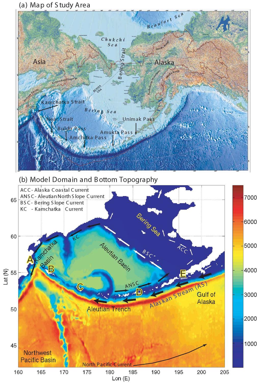
3 3 1. Introduction The Bering Sea (BS), located between Alaska in the east and Russia in the west (Fig. 1) plays an important role in the global ocean circulation and climate change. It provides the only connection (through the Bering Strait) between the Pacific Ocean to the south and the Arctic Ocean to its north. The northeastern part of the BS is a wide and shallow (depth < 200 m) continental shelf, while the southwestern portion (known as the Aleutian Basin) is deep (up to 3500 m); a strong northwestward Bering Slope Current (BSC, Fig. 1b) is observed between the two [e.g., Johnson et al., 2004; for reviews of the circulation and physical oceanography of the BS see Takenouti and Ohtani, 1974; Royer and Emery, 1984, Stabeno et al. 1999, and others]. The BS ice coverage and ecosystem is affected by global climate change and by long-term Pacific Ocean decadal variability [Jin et al., 2009]. Seasonal and interannual variations in the atmospheric pressure system over the North Pacific may impact storm tracks and possibly ocean gyres over the BS [Pickart et al., 2009]. Models and observations also suggest that the Bering Strait flow can play a crucial role in the global ocean overturning circulation and long-term climate changes in the Atlantic and Pacific Oceans [De Boer and Nof, 2004; Keigwin and Cook, 2007]. The interaction of the BS with the adjacent basins depends on the (northward mean) flow through the narrow and shallow Bering Strait which connects it to the Chukchi Sea in the north, and flows through several passages along the long chain of the Aleutian Islands in the south. While long-term currents and transports through the Bering Strait have been measured for some time [Aaagaard et al., 1985; Coachman and Aaagard, 1988; Roach et al., 1995; Woodgate et al., 2005, 2006], observations of the

4 4 transports through the Aleutian Island passages are more sparse and limited to a few main passages [Favorite, 1974; Reed, 1990; Reed and Stabeno, 1993; Stabeno and Reed, 1992; Stabeno et al., 2005; Panteleev et al., 2006; Ladd and Stabeno, 2009]. The main Aleutian passages are, from east to west [see Stabeno et al., 1999, 2005 for details], Unimak Pass, Amukta Pass, Seguam Pass, Amchitka Pass, Buldir Pass, Near Strait and Kamchatka Strait (Fig. 1a); they are generally shallower in the east and deeper in the west. Only the easternmost connector, Unimak Pass, allows significant northward flow of shelf water (the Alaskan Coastal Current, ACC; Fig. 1b) to enter directly into the BS shelf. While the flow in Unimak Pass seems uniform across the shallow (~100 m) pass, the other passages often have flows into the BS along the eastern side of the pass and return flows out of the BS along the western slope of the pass [Stabeno et al., 1999]. The westernmost and deepest passage (sill depth > 4000 m), the Kamchatka Strait, is the only passage with a dominant southward surface intensified flow (the Kamchatka Current, KC; Fig. 1b) along the continental slope; deep return flows into the BS is found on the eastern side of the strait [Stabeno et al., 1999]. Northward transports through these passages can vary from one passage to another (from ~0.1 Sv to ~15 Sv; 1 Sv = 10 6 m 3 s -1 ) and have variations on time scales ranging from days to seasonal and interannual [Reed and Stabeno, 1993; Stabeno et al., 2005]. The variability of the flow in individual passages is often an order of magnitude larger than the mean, for example observations in Amchitka Pass show a mean transport of ~0.3 Sv northward, but a range of ±3 Sv [Stabeno et al., 1999]. Moreover, mean transport based on observations may not be very accurate since most observations done in this region cover only the upper 1000 m and do not extend to measure deep, near-bottom currents. One wonders if inflow/outflow variations are merely

5 5 redistributed through different passages with no significant influence on the BS, or if there is a net cumulative effect that may change the BS circulation and balance of mass and energy. We will use a numerical model to investigate the relation between transports across different passages. Previous high resolution numerical simulations of the variability of flows through the Aleutian Islands by Overland et al. [1994] show the complex nature of these flows. However, their model had only three vertical layers and did not include the Bering Sea shelf. We will use here a more realistic model that extends from the shelf to the deep ocean and has high horizontal and vertical resolutions. The variations of transports through the Aleutian passages are especially complex because of the strong variability and limited direct observations of the Alaskan Stream (AS, Fig. 1b). The AS is the northern boundary of the Pacific subarctic gyre, flowing westward at speeds reaching in some places over 1 m s -1, from the Gulf of Alaska, along the southern edge of the Aleutian Islands Arc and toward the western North Pacific basin. There are evidence from observations [Reed, 1984, 1990; Stabeno and Reed, 1992; Reed and Stabeno, 1993; Stabeno et al., 2005] and models [Liu and Leendertse, 1982; Maslowski et al., 2008] that waters from the AS enter the BS and that flow through the passages are strongly influenced by variations in the AS transport. Reed and Stabeno [1993] show that the AS turned north and entered the Near Strait in the western Aleutian Islands in some years, while during other years Stabeno and Reed [1992] found an anomalous AS path, where it turned south and did not pass through the Near Strait. Stabeno et al. [2005] show correlations between low-pass filtered transports at Amukta Pass in the eastern Aluetian Islands and the AS transport. In addition to the northward deflection of the AS into the BS, observations [Favorite, 1967; Stabeno and Reed, 1992]

6 6 and models [Overland et al., 1994] indicate that the AS separates southward at various locations, perhaps as a result of conservation of potential vorticity along the curved island chain [Thomson, 1972]. Measuring the AS transport and position is difficult because of the influence of mesoscale eddies [Overland et al., 1994; Crowford et al., 2000; Maslowski et al., 2008], so estimates of the AS transport range from 8-25 Sv, based on upper ocean observations [Reed and Stabeno, 1999], to 28 Sv, based on full water column observations [Waren and Owens, 1988], or even up to Sv as inferred from models and altimeter data [Maslowski et al., 2008]. An AS transport of 25 Sv is used in our model for the control case; this value is considered a reasonably mean transport given the large discrepancy between the different studies [Pickart et al., 2009]. The Stream is believe to have seasonal variations associated with the seasonal pressure system and related variations in the circulation in the Gulf of Alaska [Reed, 1968; Brower et al., 1977; Royer, 1975; Cummins, 1989; Pickart et al., 2009], though some observations do not show evidence of seasonal change in AS transport [Favorite, 1967; Reed and Stabeno, 1999]. While observations and models show clearly that the AS impacts the exchange of waters between the BS and the Pacific Ocean, it is not clear how the AS influences the BS climate. Can the impact of the AS be felt farther north, affecting the Bering Strait through flow toward the Chukchi Sea, and thus potentially influencing the Arctic and the Atlantic oceans climate? The observed variability of the Bering Strait transport has dominant seasonal cycle [~0.8 Sv mean and ~ Sv variations, Coachman and Aagaard, 1988; Woodgate et al, 2005] associated with the seasonal wind pattern, but variations of fresh waters associated with the fresh and warm ACC in the eastern BS may

7 7 also be important [Woodgate and Aagaard, 2005; Woodgate et al., 2006]. Interannual variations in the Bering Strait transports [Coachman and Aagaard, 1988] are typically ~0.1 Sv, but at times can reach up to ~50% of the mean [Roach et al., 1995]. Some observations that indicate long-term Bering Strait mean transport of less than 0.6 Sv [Aagaard et al., 1985] may reflect interannual variations. Because of the dominant role of the Bering Strait fluxes on Arctic ice and climate, it is important to understand the mechanisms influencing its dynamics and variability. The goal of our study is to understand the role of the mean AS transport and its mesoscale variations in affecting the BS-Pacific Ocean water exchange across the Aleutian Islands and its potential impact on the Bering Strait outflow from the BS into the Arctic Ocean. To isolate the AS impact from other dominant factors like tides, seasonal sea-ice variations, fresh water and wind patterns, etc., we will use a numerical model with an idealized forcing that includes only lateral transports with different AS transports. The two main questions we try to answer are: 1. How do the mean transport of the Alaskan Stream affect the dynamics of the Bering Sea? and 2. How much of the observed variability in transports exchange between the Pacific-Bering-Arctic system can be attributed to mesoscale variations in the AS, when there is no time dependent forcing in the system. The paper is organized as follows: section 2 describe the model setting and the experiments performed, section 3 analyses the model results for the different experiments and section 4 offers discussion and conclusions. 2. Model setting and sensitivity experiments

8 8 The numerical model is based on the Princeton Ocean Model (POM) code [Mellor, 2004; for the latest version see which is a terrain-following (sigma-coordinates), free surface, primitive equation ocean circulation model. The model includes the Mellor and Yamada [1982] turbulence closure scheme for vertical mixing coefficients. The Bering Sea configuration of the model with realistic surface forcing and various data assimilation modules [Oey et al., 2005; Lin et al., 2007] is part of an ongoing climate and ecosystem modeling studies [Wang et al., 2003; Jin et al., 2009]. However, in the study presented here, only simplified forcing is used in order to isolate the role of the Alaskan Stream transport. Therefore, in this study there is no data assimilation, no sea-ice, no tides, no winds and zero surface heat/salt fluxes. In fact, there is no any time-dependent forcing in the model, so all the variations in the flow are internally generated by current instability and generation of mesoscale eddies. The horizontal model grid cells are Δx ~ 5km and Δy ~ 8km. The sigma coordinate (scaled over the water column) in the vertical has 51 layers with higher resolution near the surface and bottom. The model domain and bottom topography are shown in Fig. 1b. Open boundaries include radiation boundary conditions that allow the baroclinic flow to adjust to the density field. In the analysis of area averaged properties the regions within a few degrees near the south, east and west open boundaries will be ignored, but not the area near the north boundary where the outflow dominated boundary have only small impact on the interior.

9 9 The only imposed conditions on the lateral boundaries are the total (surface to bottom) inflow transport that include the Alaskan Stream (AS in ) on the eastern boundary, outflow (AS out ) through the western boundary in the western Pacific Ocean, and outflow to the Chukchi Sea (CS out ) north of the Bering Strait on the north boundary. In all the experiments CS out ~0.5 Sv and AS out = AS in - CS out, whereas different values of AS in are imposed in each experiment (but held fixed throughout the integration) as described below ( AS will be used to denote the AS transport, dropping the in ). Note that the northward transport, CS, is below most Bering Strait mean transport estimations of ~0.8 Sv (though during some years transports less than ~0.6 Sv are found, Aagard et al., 1985). One should keep in mind that the model s transport in the Bering Strait neglects contributions from fresh-water and wind driven forcing and the focus here is on variations around the prescribed mean, not on getting a realistic mean. Note that the radiation boundary conditions allow a dynamic adjustment of the flow, so for example, the prescribed CS out = 5 Sv in the north, resulted in a Bering Strait net transport that varies from ~0.05 Sv to ~6 Sv with mean of ~0.35 Sv (see discussion later). Experiments with AS values from 5 to 40 Sv have been tested, but here we describe 3 experiments: 1. AS=10Sv, 2. AS=25Sv and 3. AS=40Sv; they represent values below average, around observed average and high transports, respectively. The experiments start from annual mean climatological temperature and salinity as initial conditions [based on the latest World Ocean Atlas, 2005; Locarnini et al., 2006], followed by a 12-years spin-up period. The analysis for each experiment includes daily fields obtained from a 1-year period at the end of the spin-up. With constant forcing, the model has reached a quasi-steady state

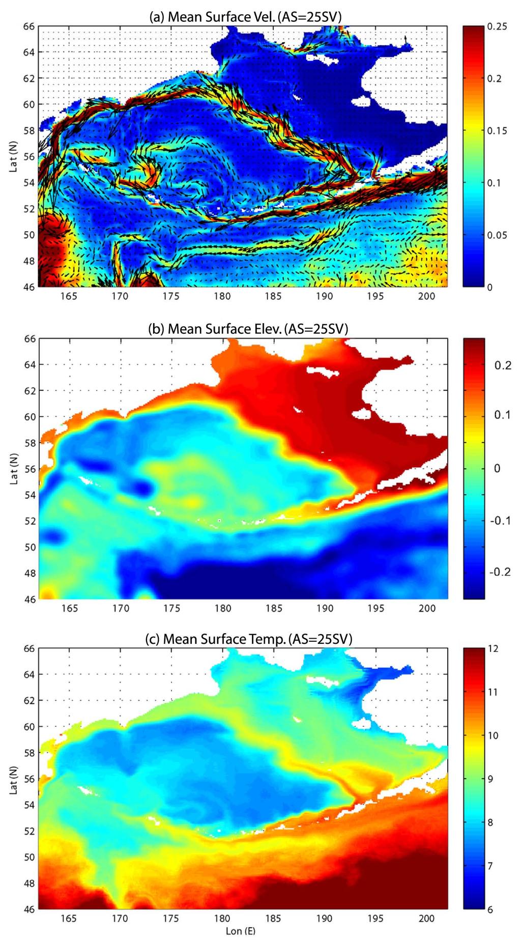
10 10 with no apparent climate drift, but has mesoscale variations generated internally in the model interior mostly due to variations in the AS. 3. Results 3.1. Mean model circulation Despite neglecting realistic forcing and seasonal variations, the model reproduced the main observed features of the general circulation in the Bering Sea [Favorite, 1974; Takenouti and Ohtani, 1974; Brower et al., 1977; Royer and Emery, 1984; Stabeno et al., 1999] quite well; Fig. 2 shows the annual mean of velocity, sea surface height and temperature for case AS=25Sv. The velocity (Fig. 2a) shows the AS flowing westward south of the Aleutian Islands with decreasing speed, as some of its surface warmer waters flow north (see the warm plumes in the temperature, Fig. 2c) through the Aleutian passages to form the Aleutian North Slope Current, ANSC [Stabeno et al., 2009]. The ANSC turns north to form the Bering Slope Current, BSC [Stabeno et al., 2009], part of which turns toward the Bering Strait and the rest forms the Kamchatka Current, KC [Panteleev et al., 2006] which flows south back into the Pacific Ocean through the Kamchatka Strait. Near the surface, the BSC is approximately in geostrophic balance with higher sea level in the Bering Sea shelf east of the BSC and lower sea level in the Aleutian Basin west of the BSC (Fig. 2b). Note that the higher sea level in the BS compared to the Arctic Ocean is an important factor in driving the northward flow through the Bering Strait [Stabeno et al., 1999], thus our results (shown later) of the

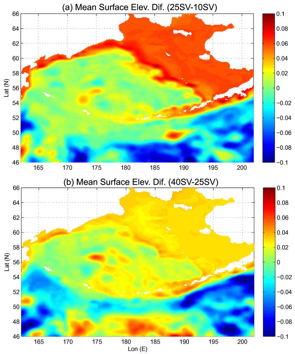
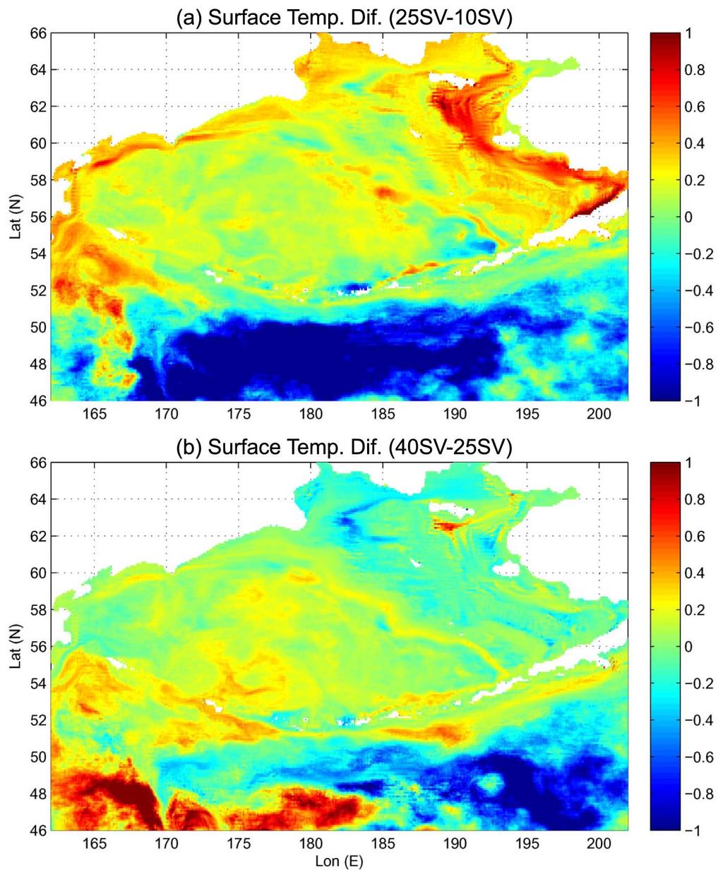
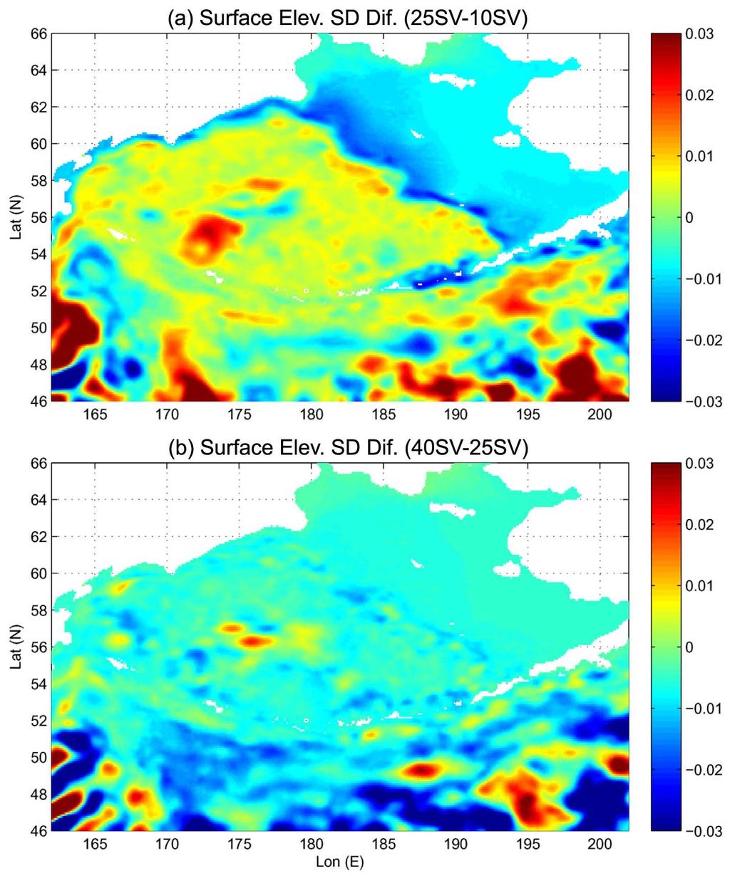
11 11 impact of AS transport on BS sea level may have implications for the Arctic Ocean climate. Note that in addition to the well documented northward branches of the AS, it also separates southward at several locations (e.g., near 180ºE and 193ºE in Fig. 2a), a phenomenon indicated in observations [Thomson, 1972; Favorite, 1974; Stabeno and Reed, 1992] and models [Overland et al., 1994] Spatial variations induced by the Alaskan Stream Transport To evaluate the spatial impact that the AS transport has on the BS, differences between different model experiments are shown for the mean fields (Fig. 3 and Fig. 4) and for the variability (Fig. 5). If the impact of the AS transport on the BS is linear, the changes when the AS transport increases from 10 Sv to 25 Sv should have the same trend as when it increases from 25 Sv to 40 Sv, however, this is not the case. The most noticeable change when the AS transport increases is the increase in mean sea level over the BS shelf (Fig. 3). As will be shown later, the increase in BS sea level also increases the geostrophic flow of the BSC and the northward flow through the Bering Strait. When the AS transport changes from 10 Sv to 25 Sv (Fig. 3a), this impact on sea level is especially large and results in warming (~0.5ºC, Fig. 4a) along the eastern shelf that is consistent with increase of transport of warm waters by the ACC. However, further increased AS transport from 25 Sv to 40 Sv causes a slight cooling of the BS shelf (Fig. 4b). The cooling is larger in the northern shelf ( ºE, 62ºN), caused by a weakening of the northward branch of the BSC as it turns south to form the KC. As the AS becomes more inertial, the area of impact on the Aleutian Islands

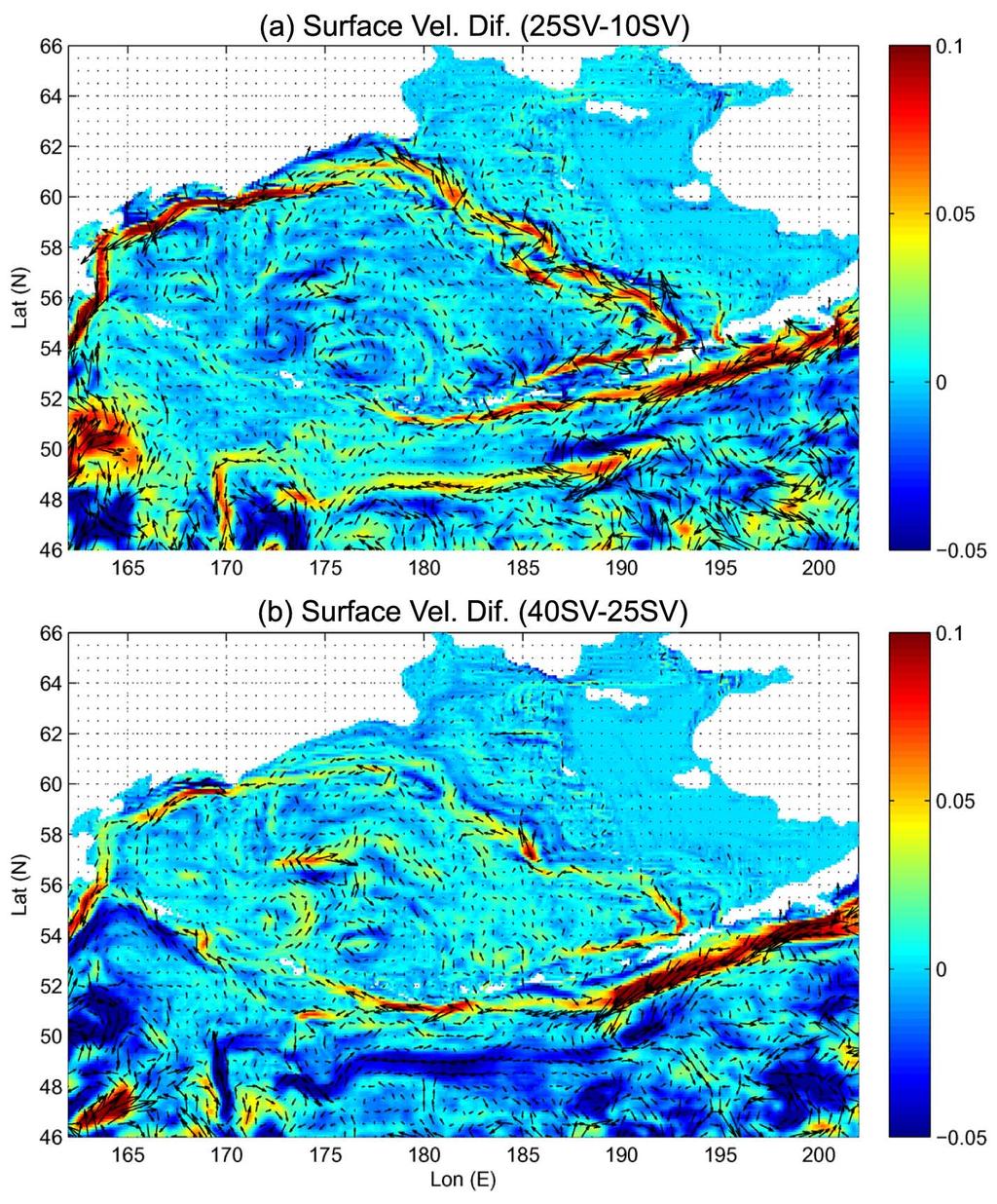
12 12 region is shifted farther downstream (westward), as seen in the surface elevation gradients between the Aleutian Basin and the Pacific Ocean (Fig. 3a versus Fig. 3b) and in the warming seen west of 180ºE when AS transport increases from 25 Sv to 40 Sv (Fig. 4b). The non-linear BS response to the AS transport is also noticeable in the change in sea surface height variability (Fig. 5). When AS transport increases from 10 to 25 Sv, the BS shelf variability decreases but the Aleutian Basin variability increases (Fig. 5a). However, a further increase of AS transport from 25 Sv to 40 Sv results in overall decrease in variability almost everywhere. There seem to be a threshold in which mean currents dominate over mesoscale variability in the model. The changes in surface flow between the experiments are shown in Fig. 6. Increasing the AS transport from 10 to 25 Sv intensifies the ANSC, the BSC and the KC (Fig. 6a), while increasing the AS transport from 25 to 40 Sv results in increasing flows farther to the west near the western Aleutian passages Temporal variations and water exchange through passages The model domain is divided into three different regions according to the topography (Fig. 1b): 1. Bering Sea shelf, 2. Aleutian Basin and 3. Northwest Pacific Basin; (1) and (2) are separated by the BSC and (2) and (3) by the Aleutian islands. Note that there is only one direct connection between (1) and (3), Unimak Pass, but many passages between (2) and (3). Area averaged sea surface height (SSH) and kinetic energy per mass (KE= 2 2 u + v ) over each of the three sub-regions are calculated from the daily

13 13 model output and shown in Fig. 7. The regions near the model boundaries, within ~3 longitude degrees in the east and west and ~3 latitude degrees in the south, were ignored. If there is a correlation between, say increased SSH in one sub-region and decreased SSH in adjacent basin, it will indicate a net transport of water between the basins. For example, given the area of the BS shelf in the model (~600,000 km 2 ), a gain of 15 cm in SSH over a 10 day period translates to ~0.1 Sv of net inflow transport into this region. Although the model does not have any time-dependent forcing, there are noticeable temporal variations associated with mesoscale and basin-scale variations. Large variations in SSH are especially apparent over the BS shelf, but they decrease as AS transport increases (Fig. 7a-c); they are equivalent to up to ~0.1 Sv net gain/loss. The BS shelf SSH is highly correlated with the inverse of the Pacific SSH (correlation coefficient R~-0.9) for all experiments, but the Aleutian Basin SSH is highly correlated with the inverse of the Pacific SSH (R~-0.7) only for AS transport over 25 Sv. The latter result is consistent with the previously discussed idea that increasing AS transport shifts the variability farther west, i.e., affecting the Aleutian Basin in the central and western BS more than the eastern shelf area. The increase in the annual mean SSH over the BS, as seen in Fig. 3) is also evident here. In contrast to the SSH anti-correlations, the area averaged surface kinetic energy in the BS (right panels of Fig. 7) have positive correlations with the Pacific Ocean, but they are significantly higher for a weaker AS (R~0.6 for AS=10Sv, but R<0.3 for AS=25Sv). Therefore, for AS=10Sv when KE increases in the Pacific Basin (say between days , Fig. 7d) it also does so for the BS, but no similar response is seen for the other two cases, AS=25Sv or AS=40 Sv (Fig. 7e and Fig. 7f). The implication is that BS

14 14 variability may be more sensitive to mesoscale variations during years with relatively weaker AS. The correlation between area-averaged properties in the BS and the Pacific Ocean indicates transport exchanges across the Aleutian Islands. The Aleutian Islands Arc stretches for some 3000 km with 30 or more passages; only few passages have been explored [Stabeno et al., 2005]. Therefore, we do not attempt to analyze the flow through all the passages. Instead, we first examine transports across 4 large sections (defined in Fig. 1b), then we will study more closely the model variability in a few passages that have been observed. The annual mean maximum surface velocity and total transports across the 4 sections are shown in Fig. 8a and Fig. 8b, respectively. The surface velocity is in general agreement with observations: flow enters the BS from the eastern and central passages and exit through the Kamchatka Strait. For example, the strong southwestward flow in section A-B is consistent with the observed direction and speed of the KC [Panteleev et al., 2006], and the north-eastward inflow in section C-D is consistent with the currents observed through the Amchitka Pass [Reed, 1990]. The surface flow in all the sections increases when the AS transport increases. The interpretation of the total model transports across the sections (Fig. 8b) is more difficult, as the variability (thin black lines) is often larger than the mean (color thick arrows). With increasing AS transport the variability in transports is reduced and so is the net transport, except the easternmost shallower section D-E. The mean transports through many passages are not well known, and large discrepancies often found in estimates based on different observations, therefore, quantitative model-data comparisons are very difficult to do (see more on this later when comparing the model with

15 15 observations at specific passages). The model means in A-B and in C-D are not in agreement with previous estimates, but given the idealized forcing (e.g., no wind-driven circulation) the model is not expected to exactly reproduce the observations. In particular, the model produces strong deep currents that seem to balance the upper ocean flow, but long-term near bottom currents have not been measured in many passages. Deep inflows into the BS in most passages are assume to exist, usually along the eastern slope of each pass [see Fig. 3 in Stabeno et al., 1999], but their transports are not well known. Net transports from the Pacific Ocean into/out-from the BS must be balanced by either raising/dropping BS sea level or by out/in flow to the Arctic Ocean through the Bering Strait (there is no water fluxes by rivers or through the air-sea interface in the model). Therefore, the linear correlation between the transports at the 4 Aleutian sections and the transport of the Bering Strait is calculated from the daily data and shown in Fig. 8c. Generally, when inflow transports through the eastern Aleutian Islands increase, the northward Bering Strait transport increases (positive correlations with sections C-D and D-E) and the southward outflow through the Kamchatka Strait increases (negative correlation with section A-B). Section A-B and C-D are also highly correlated with each other (Fig. 9). Correlations are much higher for AS=10Sv than for the other experiments, which is consistent with the reduction of variability for stronger AS (Fig. 7 and Fig. 8b). The relation of the mesoscale variations in transports across the Aleutian Island sections are shown in Fig. 9. Again, it is apparent the variability decreases when AS transport increases. The largest variations (up to Sv) are in sections A-B and C-D which nicely balances each other, i.e., net inflow/outflow around Amchitka Pass corresponds to

16 16 outflow/inflow through Kamchatka Strait. Variations in the other sections are smaller, but not negligible (~5 Sv). An important question is whether the transports through the Aleutian passages merely balance each other as seems in Fig. 9, or there is a net imbalance that can impact the BS? Such imbalance can contribute to sea level variations in the BS and potentially to variations in the Bering Strait transport. Fig. 10 shows the Aleutian transport versus the Bering Strait transport for the three experiments. The Aleutian-Bering Strait correlation is slightly higher when the Bering Strait transport lags by 2-days behind the Aleutian transports. This lag is of the order of the time it takes a barotropic wave to propagate around the BS (they slow considerably over the shallow shelf). When the AS transport increases, the Aleutian-Bering Strait correlation slightly increases, but the variability of the Bering Strait transport decreases; the standard deviations of the Bering Strait transport is 0.1Sv, 0.09Sv and 0.08Sv for AS=10Sv, 25Sv and 40Sv, respectively. The sensitivity of the Bering Strait transport to changes in the Aleutian transports (the slope of the linear regression fit line in Fig. 10) is also a monotonic function of the AS transport, but on average, an increase of ~3 Sv in the Aleutian net transport into the BS will cause ~1 Sv increase in the Bering Strait transport (and the rest, ~2 Sv, will contribute to changes in BS total volume, thus in sea level). Note that the model variations in the Bering Strait transport of ~±0.3 Sv (Fig. 10) are comparable to the observed interannual variations in the Bering Strait transport over ~30-year period (Coachman and Aagaard, 1988), so even a small imbalance in the Aleutian transports may be significant in terms of its long-term impact on transports toward the Arctic Ocean.

17 17 The variations in volume transports shown in Figures 8-10 would also have important implications for heat exchange between the Pacific Ocean, the Bering Sea and the Arctic Ocean. The idealized model does not include surface heat fluxes to allow calculations of complete heat budgets, nevertheless, the experiments indicate how the AS transport may impact the heat transports in/out of the BS. Observation-based estimates of heat transports are available for the Bering Strait, but not for the Aleutian passages. The mean northward heat transport through the Bering Strait in the model is around 0.01 PW (1 PetaWatt=10 15 Watt) or ~3.1x10 20 J y -1. In comparison, Woodgate et al. [2006] estimated the heat flux in the Bering Strait to vary between 1-3x10 20 J y -1 with considerable interannual variations. The lack of surface heat loss over the BS in the model should result in heat fluxes larger than observed through the Bering Strait, so despite the underestimated volume transport in the model, the heat transport is quite reasonable for this idealized experiment. The heat flux through the Bering Strait increases by ~15% when the AS transport increases from 10 to 25 Sv, but decreases by ~5% when the AS transport increases from 25 to 40 Sv; this result is consistent with the heating and cooling of the BS shelf seen in Fig. 4a and Fig. 4b, respectively. Woodgate et al. [2006] estimated that ~1/3 of the warming and increase in heat flux through the Bering Strait between 2002 and 2004 can be attributed to the ACC. As for the heat flux through the Aleutian passages, the largest change between the 3 experiments occurred in the eastern passages (across section D-E, Fig. 1b), where northward mean heat transports of , and PW were found for experiments 10, 25 and 40 SV, respectively (an increase of ~53% and 11% between the experiments). These changes would affect the heat transports by the ACC and BSC, and thus likely impact the heat flux through the

18 18 Bering Strait, as suggested by Woodgate et al. [2006]. The increased heat transport into the BS across the eastern Aleutian passages when the AS transport increases is balanced in the model by an increased of heat transport out of the BS through the Kamchatka Strait. However, these changes would also affect the air-sea heat exchange and sea-ice formation over the BS; such processes are neglected here, so further discussion of the net heat balance in the BS are left for follow up studies with more realistic forcing Comparison with observed transports Since the model forcing is idealized: no wind, no tides, no sea-ice nor any timedependent forcing, and consists of only forcing by constant lateral transports, comparisons with observations may tell us what portion of the observed variability is forced by the AS and mesoscale variability generated by internal dynamics. Over the years, observations of transports have been taken across some of the Aleutian Island passages and more consistently in the Bering Strait; some of these observations are summarized in Table 1 and compared with the model experiments. Note that the 6 major Aleutian passages included in Table 1 may have been observed more than others, but nevertheless are only part of the many [~30; Ladd and Stabeno, 2009] passages, thus the total transport in Table 1 is not expected to be balanced. In fact, comparing the sum of the 6 Aleutian transports in Table 1 with the transport of all passages in Fig. 8 indicates ~4-5 Sv of missing outflow transports (i.e., in passages not included in Table 1). Close examination shows that the missing transports are distributed as follows: (1) ~2.5 Sv additional southward transport is found in section B-C (Fig. 1b), probably around Near

19 19 Strait. This can explain the relatively low net transport in the model s Kamchatka Strait. (2) ~3 Sv additional southward transport is found in section C-D near Buldir and Amchitka Passages. This region has been poorly observed and often show southward flows ([Stabeno et al., 1999]. (3) ~1.5 Sv additional northward transport is found in section D-E. This transport may include the Akutan and Samalga passages [~0.5 Sv total; Ladd and Stabeno, 2009] east of Amukta Pass as well as additional inflow in unobserved eastern passages. Therefore, the total transport in the eastern passages that feed the ANSC is actually closer to observations than the impression given by the low model s transport in Amukta Pass. It is noted that very recent estimates of the transport through Amukta Pass [4.7 Sv; Ladd and Stabeno, 2009] are significantly higher than previous estimations. Since the model forcing is idealized, discrepancies from observations are expected. However, it is also clear that there is little consensus of the transport across most passages between different observations and estimates vary sometimes by an order of magnitude. In some cases the direction of the mean transport vary between one observation to another, especially for deep passages like Amchitka where transports range from ~3-4 Sv outflow to 2-5 Sv inflow [Reed, 1984, 1990; Stabeno et al., 1999]. The problem relates to lack of deep observations, the large mesoscale variability and interannual variations that cause unusual transports in some years [Stabeno and Reed, 1992; Reed and Stabeno, 1993]. The model mean transports and variability are in general in better agreement with observations across shallower passages than in deep western passages (e.g., Near and Kamchatka Straits). Interestingly enough, in one of the least explored passages, Buldir Pass, the model actually show large inflow transport (~4-5 Sv).

20 20 Until there are long-term, high resolution direct velocity observations that extends all the way from the surface to the bottom (over 4000 m in Kamchatka Strait) it will be difficult to quantitatively assess the model results. Note that velocity and transport estimates from temperature and salinity casts often assume a level of no motion at say 1500 m depth, but as will be shown later (Fig. 11), flow in straits often have strong near-bottom currents, so such assumptions may not be correct. The model suggests that a large part of the discrepancy between various observations may be attributed to mesoscale variability since the standard deviation of transports is large compared with the mean. In the deep straits, variability of model transport is ~±4-8 Sv compared with ~1-3 Sv mean transport. The impact of the AS transport on the mean and variability is different for each passage, for example, there is little impact on the transport through Amchitka Pass and Near Strait, but when AS transport increases from 10 Sv to 40 Sv, the net transport in Kamchatka Strait is changed from small inflow to small outflow. The stronger observed southward transport in Kamchatka Strait [Panteleev et al., 2006] can be partly attributed to the southward seasonal wind pattern along the coast of Asia [Pickart et al., 2009]; as mentioned before, the model neglects this forcing. In the Bering Strait, the transport variability is about 30% of the mean, though it should be acknowledged that the model mean is low compared to observations, as it largely depends on the imposed northern open boundary conditions, and does not include a wind-driven component which is known to control Bering Strait flow variability [Coachman and Aagaard, 1988; Woodgate et al., 2005]. To quantify the impact of the AS transport on different passages in comparison with mesoscale variability, an impact factor is defined as the ratio between the range of

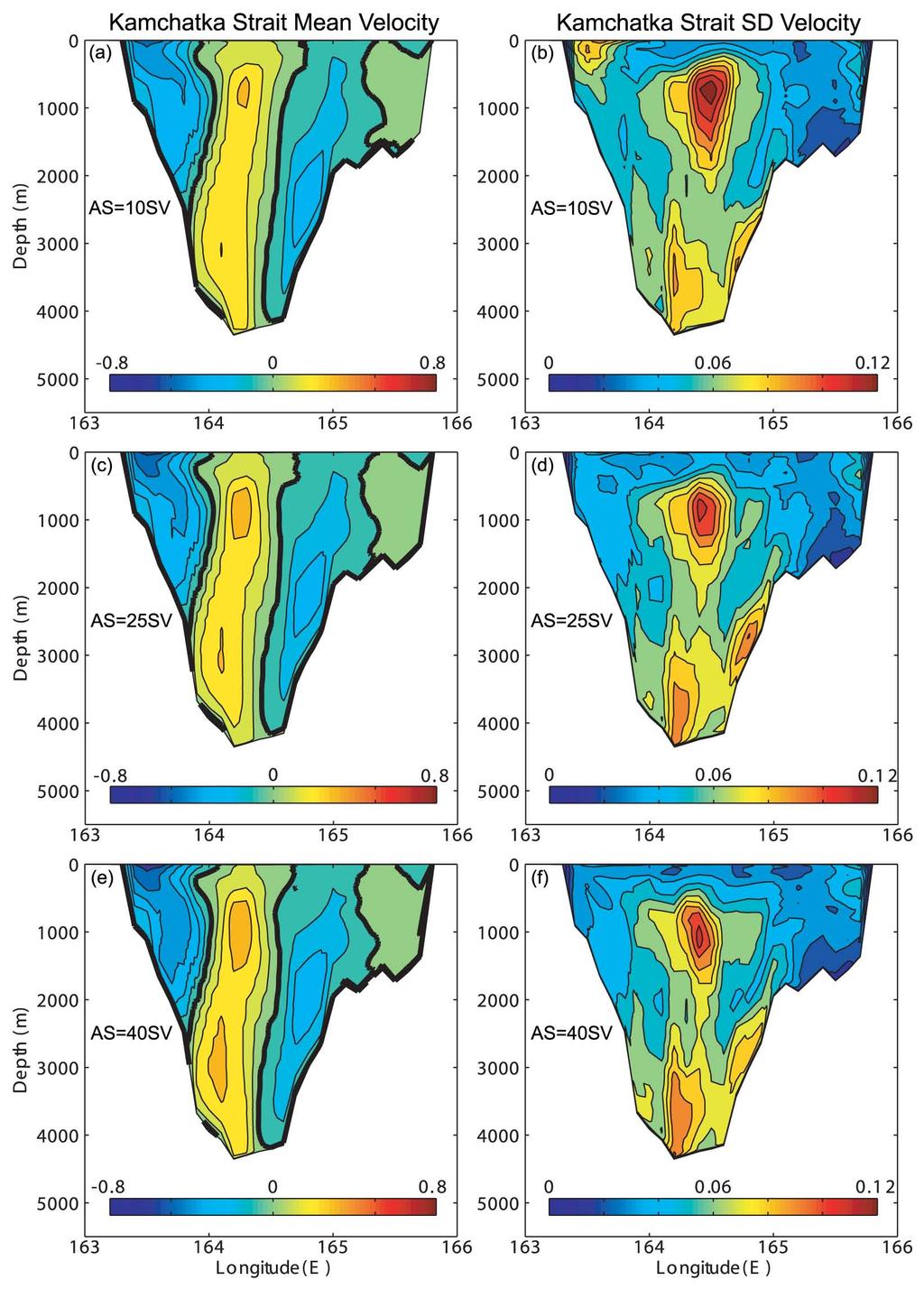
21 21 transport variations between the three experiments and twice the average standard deviation of the mesoscale variations (last column in Table 1). In the relatively shallow passages (Unimak, Amukta and Buldir) and in the outflow of Kamchatka Strait, climatic changes in the AS transport may contribute to the variability the equivalent of ~30% of the mesoscale variability. The variability ratio factor is surprisingly similar in these 4 passages located thousands of kilometers from each other. The two deep inflow passages (Near Strait and Amchitka) seem to have different variability ratios, whereas mesoscale variations dominate over climatic AS transport variations (which contribute only 4-12% of the variability). The latter may explain the conflicting transport estimates between different observations taken at these two passages [Reed, 1984, 1990; Stabeno and Reed, 1992; Reed and Stabeno, 1993; Stabeno et al., 1999]. Kamchatka Strait seems to stand out as a place where the model mean transport (~3 Sv net inflow in AS=10Sv to ~1 Sv net outflow in AS=40Sv) appears to disagree with most observations that estimate a net outflow of 5-15 Sv due to the southward flowing Kamchatka Current [Stabeno et al., 1999]. Therefore, the velocity and variability across this strait for the three experiments are shown in Fig. 11. The observed strong outflow of the Kamchatka Current along the western coast of the strait is well reproduced in the model (~25 Sv), but the model flows at the deep (water depths > 4000 m) portion of the strait (left panels of Fig. 11) have not been observed (only very limited number of measurements are available in such deep waters). Therefore, the model results suggest that estimations of total transports in the strait based on upper ocean observations may not be accurate. In the model, a barotropic inflow occupies the center of the strait from ~ m, and a deep outflow is seen along the eastern slope of the strait centered

22 22 around 2000 m depth. The outflow region is where most of the variability occurs (right panels of Fig. 11), with a maximum standard deviation of ~0.15 m s -1 found at 500 m depth in the center of the strait. Since the model neglects wind variations, there are almost no variations in the currents at the upper ~500 m. The impact of the AS transport is to increase both the KC outflow and the return inflow. However, the former is increased more than the latter due to the net increase of inflow transports through the Aleutian passages, resulting in an increased net Kamchatka Strait outflow as the AS becomes stronger. As seen before, the variability decreases with increasing AS transport. It is especially noticeable that significant variability in the Kamchatka Current is only seen for the AS=10Sv experiment (Fig. 10b). Since to our knowledge there are no observations at 4000 m in the Kamchatka Strait that can verify if the model results are real or not, we have only found some anecdotal evidence that this flow pattern may be plausible. For example, using hydrographic and drifter data, and inverse calculations, Panteleeve et al. [2006] found that the transport of the Kamchatka Current is about twice as large (~24 Sv) than previous estimates. Our results show ~25 Sv outflow in the Kamchatka Current plus ~7 Sv deep outflow along the eastern slope, which are balanced by ~32 Sv deep inflow. Weaker Kamchatka Curreent estimates of 6-11 Sv by Verkhunov and Tkachenko [1992] and others were based on dynamic height calculations relative to 1000 or 1500 m; based on the model results, the assumption that there is no flow below 1500 m is incorrect. Temperature distribution observed at m depth north of Kamchatka Strait sometimes shows a plume of slightly warmer waters northeast of the eastern side of the strait [see Fig. 6c in Verkhunov and Tkachenko, 1992], which could indicate a subsurface

23 23 warmer inflow from the Pacific. Reviewing various observations, Stabeno et al. [1999] describe inflow of Deep Pacific Waters (DPW) below 2000 m, entering the BS near the eastern side of the Kamchatka Strait. This deep inflow is supported by models and data calculations of the abyssal circulation in the North Pacific, for example, Morehead et al. [1997] shows that one of the most robust near-bottom flow in the northwest Pacific basin is a deep (~5000 m) boundary current flowing toward the Kamchatka Strait. An intriguing observation described in Stabeno et al. [1999] is the high concentration of silica found in the strait between m depth, suggesting the existence of (quote)... a southward flow of deep Bering Sea water beneath the Kamchatka Current and above the inflow of DPW. The deep return flow in our model is found between m (Fig. 11). The barotropic nature of the deep flows in the model and temperature sections (not shown) indicate though, that those flows may not be detected from temperature and salinity sections, but instead, direct velocity measurements are needed. 4. Summary and conclusions The Bering Sea (BS) provides an important connection between the Pacific Ocean and the Arctic and Atlantic Oceans and is subject to ongoing research related to global climate change and its impact on the rich marine ecosystem [e.g., Hunt et al., 2002; Jin et al., 2009]. The climate and variability of the BS is affected by different forcing, such as seasonal wind pattern, sea-ice, freshwater influx, etc. An important impact on the BS circulation and climate comes from the exchange of water, heat, nutrients, etc. between the BS and the Pacific Ocean through the various passages in the Aleutian Islands Arc.

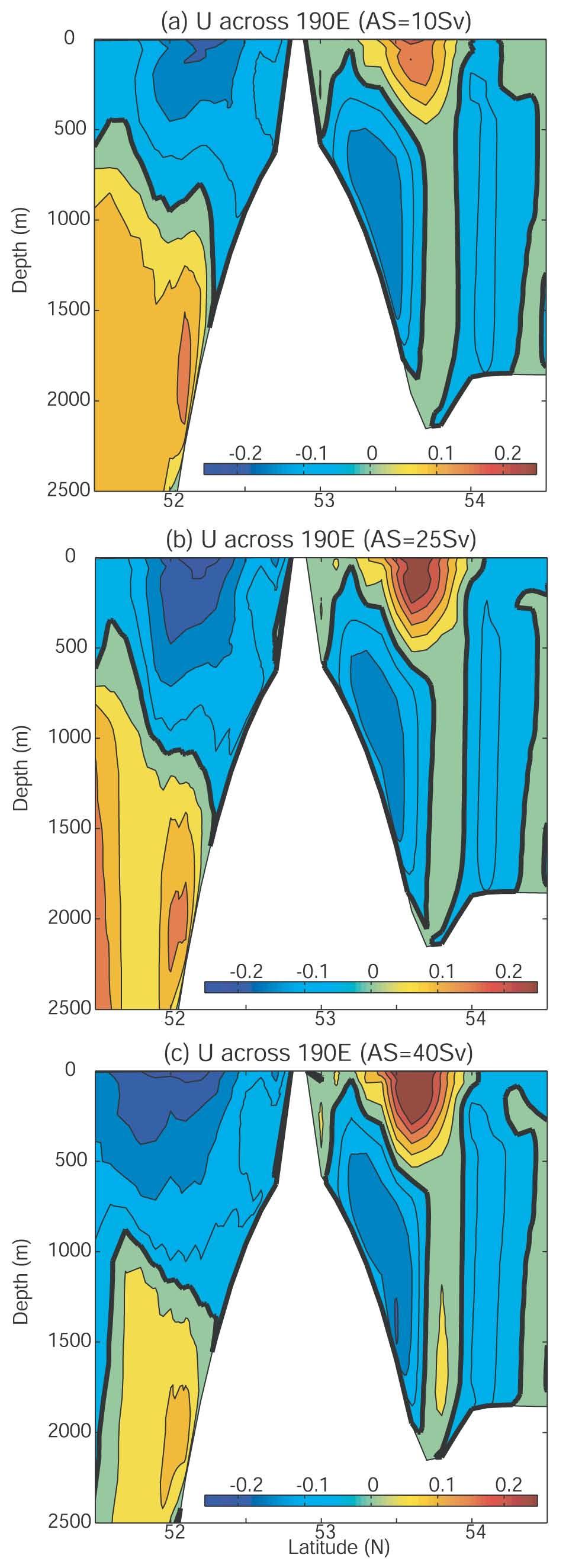
24 24 These transports are affected by the strong Alaskan Stream, AS [Reed, 1984; Reed and Stabeno, 1993, 1999; Maslowski et al, 2008]. Unfortunately, there are no long-term observations of the full water column across the AS, so numerical models may be needed to help understand its dynamics [e.g., Overland et al., 1994]. The goal of our study was thus to isolate the role of the AS in affecting the transport exchanges between the Pacific Ocean and the BS. Some important questions are: what will happen to the BS if longterm Pacific climate variations change the transport of the AS? and what part of the observed variability can be attributed to variations in the AS? To address such questions a numerical ocean circulation model with realistic topography of the BS has been constructed. The model domain extends from the North Pacific Ocean in the south to the southern edge of the Chukchi Sea in the north. The model is driven by an idealized forcing that includes only lateral transports with three different AS transports (10Sv, 25Sv and 40Sv); these transports are all within the range of different estimates based on observations. The sensitivity of the flow in the Bering Sea to variations in the AS transport are demonstrated for example in Fig. 12. This section across 190ºE, just east of Amukta Pass, shows that when the AS transport (imposed on the model boundary ~150 km upstream of this section) increases, the mean westward flow of the AS (the blue core in Fig. 12) deepens and widens, as expected. However, a more interesting result is the significant increase in the speed and extent of eastward flowing ANSC (the red core in Fig. 12). The impact of the AS on the ANSC seen here is consistent with observations [Stabeno et al., 2005] showing that the AS transport is correlated with the Aleutian passages transports that feed the ANSC. At that longitude the AS may experience considerable mesoscale eddy variability [Maslowski et al., 2008] so

25 25 the widening of the AS core seen in the annual mean velocity when its transport increases (Fig. 12) reflects wider offshore/onshore variations in its location (consistent with Fig. 5). Note that the model of Maslowski et al [2008] also show deep eastward return flows below the AS, as seen here. The model results show some unexpected findings. An increase of AS transport from 10 to 25 Sv causes a warming of ~0.25ºC over the BS shelf due to increased transports of warmer Pacific waters through the eastern passages of the Aleutian Islands, but further increase of AS transport from 25 to 40 Sv had an opposite impact on the BS shelf with a slight cooling of ~-0.1ºC (though cooling of up to ~-0.5ºC are obtained in some locations). These changes are caused by circulation changes and associated advection of different water masses. More intense (inertial) AS transport is able to impact flows through passages farther downstream in the western Aleutian Islands. Moreover, the variability in the entire BS is reduced when the AS is stronger than normal. Mesoscale variations in the AS not only affect the variability of transports across the Aleutian Islands, but also the variability of the Bering Strait flow into the Arctic Ocean; an important factor in climate variations and predictions. It is estimated that potential long-term changes in the mean transport of the AS may contribute to changes in transports across the Aleutian Islands that are about 25-30% of the contribution from mesoscale variability. However, the impact of AS transport is somewhat different for each passage, depending on its local topography and location along the Alutian Islands Arc. Therefore, future process studies will focus on the detailed flow-topography interactions across different passages. In particular, the model suggests deep return flows (in opposite direction to the upper ocean currents) that may have been previously missed.

26 26 Therefore, the total net transports calculated by the model in deep passages (e.g., Kamchatka Strait) are often different than estimated transports based on mostly upper ocean observations. The model velocity across the Kamchatka Strait (Fig. 11) is much more complex than previously inferred from (limited available) observations. Two outflow currents are found, the well known KC along the western coast of the strait, and less known middepth ( m) currents. The existence of the latter current, have been suggested by some authors, in order to explain a core of high silica in the straits [Stabeno et al., 1999]. The deep inflow of Deep Pacific Waters is thought to occupy the bottom 2000 m [Stabeno et al., 1999; Morehead et al., 1997], but in the model it seems to occupy the center of the strait between m, with transports comparable to the outflow transports. Direct velocity observations may be needed to verify the model results, as this inflow is very barotropic with little signature in the temperature field. It is interesting to note that the unusual structure of the Kamchatka Strait flow resembles to some extent the structure found by the same authors in a very different environment, in the Yucatan Channel (YC) between the Caribbean Sea and the Gulf of Mexico [Ezer et al., 2003; Oey et al., 2004]. In both cases southward flows found along the side slopes and northward flows in the center, though the surface flow in the YC case is driven by the northward flowing Caribbean Current, while here it is driven by the southward flowing Kamchatka Current. The unusual flow pattern in the YC was discovered first by numerical models before direct observations became available, so we hope that our results in the Kamchatka Strait may motivate further observations.

27 27 While realistic ocean circulation and ecosystem models are being developed to simulate present and future climates and ecosystem impacts, process oriented studies, like the one presented here, can provide important insights and improve our understanding of particular mechanisms. Acknowledgements. The research is supported by NOAA s Office of Climate Programs, through grants to ODU (award NA08OAR ) and PU (award NA17RJ2612), as part of the project Collaborative Research: Modeling Sea Ice-Ocean-Ecosystem Responses to Climate Changes in the Bering-Chukchi-Beaufort Seas with Data Assimilation of RUSALCA Measurements ; Jia Wang and John Calder of NOAA are thanked for leading this project. TE was also partly supported by NSF s Climate Process Team project and NOAA s National Marine Fisheries Service. LO is grateful to GFDL/NOAA, Princeton, where model computations were conducted. Two anonymous reviewers provided very useful suggestions that helped to improve the manuscript.

28 28 References Aagaard, K., A. T. Roach, and J. D, Schumacher (1985), On the wind-driven variability of the flow through Bering Strait, J. Geophys. Res., 90(C10), Brower. W. A., H. F. Diaz, A. S. Prechtel, H. W. Searby, and J. L. Wise (1977), Climate atlas of the outer continental shelf waters and coastal regions of Alaska: Volume II, Bering Sea. Nat. Oceanic and Atmos. Admin., Report No. 347, 443 pp. Coachman, L. K., and K. Aaagaard (1988), Transports through Bering Strait: Annual and interannual variability, J. Geophys. Res., 93(C12), 15,535-15,539. Crawford, W. R., J. Y. Cherniawsky, and M. G. G. Foreman (2000), Multi year meanders and eddies in the Alaskan Stream as observed by TOPEX/Poseidon altimeter, Geophys. Res. Lett., 27(7), Cummins, P. E. (1989), A quasi-geostrophic circulation model of the northeast Pacific. Part II: Effects of topography and seasonal forcing, J. Phys. Oceanogr., 19, De Boer, A. M., and D. Nof (2004), The Bering Strait s grip on the northern hemisphere climate, Deep-Sea Res., 51, Ezer, T., L.-Y. Oey, H.-C. Lee, and W. Sturges (2003), The variability of currents in the Yucatan Channel: Analysis of results from a numerical 0cean model, J.Geophys. Res., 108(C1), 3012, doi: /2002jc Favorite, F. (1967), The Alaskan Stream, Int. N. Pac. Fish Comm. Bull., 21, 20 pp. Favorite, F. (1974), Flow into the Bering Sea through Aleutian Island passages, In Oceanography of the Bering Sea with emphasis on renewable resources, edited

29 29 by Hood, D. W., and E. J. Kelley, Publ. No. 2, Institute of Marine Sciences, Univ. Alaska, Fairbanks, AK. pp Hunt, J. L., P. Stabeno, G. Waltersc, E. Sinclaird, R. D. Brodeure, J. M. Nappc, and N. A. Bondf (2002), Climate change and control of the southeastern Bering Sea pelagic ecosystem, Deep-Sea Res., 49, Jin, M., C. Deal, J. Wang, and C. P. McRoy (2009), Response of lower trophic level production to long term climate change in the southeastern Bering Sea, J. Geophys. Res., 114, C04010, doi: /2008jc Keigwin, L. D., and M. S. Cook (2007), A role for North Pacific salinity in stabilizing North Atlantic climate, Paleoceanogr., 22, PA3102, doi: /2007pa Ladd, C., and P. J. Stabeno (2009), Freshwater transport from the Pacific to the Bering Sea through Amukta Pass, Geophys. Res. Lett., 36, L14608, doi: /2009gl Lin, X.-H., L.-Y. Oey, and D.-P. Wang (2007), Altimetry and drifter data assimilations of loop current and eddies, J. Geophys. Res., 112, C05046, doi: /2006jc Liu, S. K., and J. J. Leendertse (1982), Three-dimensional model of Bering and Chukchi Sea, Coastal Eng, 18, Locarnini, R. A., A. V. Mishonov, J. I. Antonov, T. P. Boyer, and H. E. Garcia (2006), World Ocean Atlas 2005, Volume 1: Temperature. S. Levitus, Ed. NOAA Atlas NESDIS 61, U.S. Government Printing Office, Washington, D.C., 182 pp.

30 30 Maslowski, W., R. Roman, and J. C. Kinney (2008), Effects of mesoscale eddies on the flow of the Alaskan Stream, J. Geophys. Res., 113, C07036, doi: /2007jc Mellor, G. L. (2004), Users guide for a three-dimensional, primitive equation, numerical ocean model, Prog. Atmos. Oceanic Sci., Princeton University, 42pp. Mellor, G. L., and T. Yamada (1982), Development of a turbulent closure model for geophysical fluid problems, Rev. Geophys. Space. Phys., 20, Morehead MD, Muench RD, Bacastow R, Dewey R (1997) Potential radionuclide transport pathways from seafloor dumpsites: Kamchatka region of the North Pacific Ocean. Mar Poll Bull, 35, Oey, L.-Y., T. Ezer, and W. Sturges (2004), Modeled and observed Empirical Orthogonal Functions of currents in the Yucatan Channel. J. Geophys. Res., 109, C08011, /2004JC Oey, L.-Y., T. Ezer, G. Forristall, C. Cooper, S. DiMarco, and S. Fan (2005), An exercise in forecasting loop current and eddy frontal positions in the Gulf of Mexico. Geophys. Res. Lett., 32, L12611, doi: /2005GL Overland, J. E., M. C. Spillane, H. E. Hurlburt, and A. J. Wallcraft (1994), A numerical study of the circulation of the Bering Sea basin and exchange with the North Pacific Ocean, J. Phys. Oceanogr., 24, Panteleev, G., P. Stabeno, V. A. Luchin, D. A. Nechaev, and M. Ikeda (2006), Summer transport estimates of the Kamchatka Current derived as a variational inverse of hydrophysical and surface drifter data, Geophys. Res. Lett., 33, L09609, doi: /2005gl

31 31 Pickart, R. S., G. W. K. Moore, A. M. Macdonald, I. A. Renfrew, J. E. Walsh, and W. S. Kessler (2009), Seasonal evolution of Aleutian low pressure systems: Implications for the North Pacific subpolar circulation, J. Phys. Oceanog., 39, Reed, R. K. (1968), Transport of the Alaskan Stream, Nature, 220(16) Reed, R. K. (1984), Flow of the Alaskan Stream and its variations, Deep-Sea Res., 31(4) Reed, R. K. (1990), A year-long observation of water exchange between the North Pacific and the Bering Sea. Limnol. Oceanogr., 35(7) Reed, R. K., and P. J. Stabeno (1993), The recent return of the Alaskan Stream to Near Strait, J. Mar. Res., 51, Reed, R. K., and P. J. Stabeno (1999), A recent full-depth survey of the Alaskan Stream, J. Oceanogr., 55, Roach, A. T., K. Aaagaard, C. H. Pease, S. A. Salo, T. Weingartner, V. Pavlov, and M. Kulakov (1995), Direct measurements of transport and water properties through the Bering Strait, J. Geophys. Res., 100(C9), 18,443-18,457. Royer, T. C. (1975), Seasonal variations of waters in the northern Gulf of Alaska, Deep- Sea Res., 22, Royer, T. C., and W. I. Emery (1984), Circulation in the Bering Sea, , based on satellite-tracked drifter observations, J. Phys. Oceanogr., 14, Stabeno, P. J., and R. Reed (1992), A major circulation anomaly in the western Bering Sea, Geophys. Res. Lett., 19(16),

32 32 Stabeno, P. J., D. G. Kachel, N. B. Kachel, and M. E. Sullivan (2005), Observations from moorings in the Aleutian Passes: temperature, salinity and transport, Fisheries Oceanogr., 14(1), Stabeno, P. J., C. Ladd, and R. K. Reed (2009), Observations of the Aleutian North Slope Current, Bering Sea, , J. Geophys. Res., 114, C05015, doi: /2007jc Stabeno, P. J., J. D. Schumacher, and K. Ohtani (1999), The physical oceanography of the Bering Sea., in Dynamics of the Bering Sea, edited by Loughlin, T R., and K. Ohtani, University of Alaska Sea Grant AK-SG-99-03, Fairbanks, Ak, Takenouti, A. Y., and K. Ohtani (1974), Currents and water masses in the Bering Sea: A review of Japanese work, in: Oceanography of the Bering Sea with emphasis on renewable resources, edited by Hood, D. W., and E. J. Kelley, Univ. Wash., Seattle, WA. Thomson, R. E. (1972), On the Alaskan Stream, J. Phys. Oceanog., 2(4), Verkhunov, A. V., and Y. Y. Tkachenko (1992), Recent observations of variability in the western Bering Sea current system, J. Geophys. Res., 97(C9), 14,369-14,376. Wang, J., C. Deal, Z. Wan, and M. Jin (2003), User s guide for a Physical-Ecosystem Model (PhEcoM) in the subpolar and polar oceans, version 1, IARC-FRSGC Tech. Rep , Intern. Arctic Res. Center, Fairbanks, Alaska, 75 pp. Warren, B. A., and W. B. Owens (1988), Deep currents in the central subarctic Pacific Ocean, J. Phys. Oceanog., 18, Woodgate, R. A., and K. Aaagaard (2005), Revising the Bering Strait freshwater flux into the Arctic Ocean, Geophys. Res. Lett., 32, L04602, doi: /2004gl

33 33 Woodgate, R. A., K. Aaagaard, and T. J. Weingartner (2005), Monthly temperature, salinity, and transport variability of the Bering Strait through flow, Geophys. Res. Lett., 32, L04601, doi: /2004gl Woodgate, R. A., K. Aaagaard, and T. J. Weingartner (2006), Interannual changes in the Bering Strait fluxes of volume, heat and freshwater between 1991 and 2004, Geophys. Res. Lett., 33, L15609, doi: /2006gl

34 34 Table 1. Comparison of model transports driven only by Alaskan Stream and model boundary conditions with transports estimated from observations across various passages (see references at the bottom). All numbers are in Sverdrup units (1 Sv = 10 6 m 3 s -1 ) and positive/negative values represent northward/southward direction. Model standard deviation values are in parentheses as well as estimated observed ranges. The last column is an estimate of the relative contribution to the variability from changing the mean AS transport as a percent of the mesoscale variability = 100 x (transport range between experiments)/(twice the average standard deviation). Location Model Run (AS=) Observations AS contribution (depth, m) 10 Sv 25 Sv 40 Sv Mean/Mesoscale Unimak Pass (~100) 0.37 (0.19) 0.47 (0.21) 0.48 (0.22) , (0.1 to 0.5) 8 27% Amukta Pass (~400) 1.1 (1.4) 1.2 (0.69) 1.4 (0.7) 0.6 8, 4 9, (-0.1 to 1.4) 8 35% Amchitka Pass (~1500) -3.4 (1.0) -3.2 (0.78) -3.3 (0.75) -4 5, , 0.3 8, 2-5 2,6 (-2.8 to 2.8) 8 12% Buldir Pass (~1000) 3.8 (1.9) 4.1 (1.2) 4.8 (1.4) ~1 8 (unknown) 8 33% Near Strait (~2500) 2.94 (2.9) 2.64 (3.2) 2.74 (3.6) ~3 8,10, 5 7, 10 2 (6 to 12) 8 4% Kamchatka Strait (~4500) 2.7 (7.6) (5.5) -0.7 (4.9) -6 13, -7 7, -12 8, (-5 to -15) 8 28% Bering Strait (~50) 0.32 (0.11) 0.35 (0.09) 0.34 (0.08) 0.6 1, 0.8 3,11 (0.3 to 1.4) 8 16% 1 Aagaard et al. [1985]; 2 Favorite [1974]; 3 Coachman and Aagaard [1988]; 4 Ladd and Stabeno [2009]; 5 Reed [1984]; 6 Reed [1990]; 7 Reed and Stabeno [1993]; 8 Stabeno et al. [1999]; 9 Stabeno et al. [2005]; 10 Stabeno and Reed [1992]; 11 Woodgate et al. [2005]; 12 Panteleev et al. [2006]; 13 Verkhunov and Tkachenko [1992].

35 35 Figure Captions Fig. 1. (a) Map of the area of interest and locations of important passages. (b) Model topography (color represents depth in meters) and schematic of major currents. Transports are calculated in the passages shown in (a) and across sections between locations indicated by A to E in (b). Fig. 2. Annual mean surface model fields from the AS=25Sv run. (a) Surface velocity speed (color, m s -1 ) and vectors. (b) Sea surface height (m). (c) Sea surface temperature (ºC). Fig. 3. Change in surface elevation (in m) when AS transport increases from (a) 10 to 25 Sv and (b) from 25 to 40 Sv. Fig. 4. Change in surface temperature (in ºC) when AS transport increases from (a) 10 to 25 Sv and (b) from 25 to 40 Sv. Fig. 5. Change in annual mean variability of sea surface height (standard deviation in m) when AS transport increases (a) from 10 to 25 Sv and (b) from 25 to 40 Sv. Fig. 6. Change in annual mean surface velocity (speed in m s -1 ) when AS transport increases (a) from 10 to 25 Sv and (b) from 25 to 40 Sv.

36 36 Fig. 7. Area averaged SSH (left panels) and squared surface velocity (right panels) for the three experiments, 10Sv, 25Sv and 40Sv, from top to bottom, respectively. Color represents three sub-regions: Bering Sea shelf (blue), Aleutian Basin (green) and North Pacific (red). The correlation coefficients (from linear regression between sub-regions) are indicated. Fig. 8. Velocity and transport at the 4 sections of Fig. 1b. (a) Maximum surface current vectors obtained from the annual mean flow across the sections. (b) Vertically integrated mean north/south transports (color arrows) and standard deviation (vertical lines). (c) Correlations between the transports across the sections and the Bering Strait transport calculated from daily flows over 1 year. The three experiments with AS transport of 10/25/40Sv are marked by red/green/blue, respectively. Fig. 9. Time series of daily transports across the four Aleutian Islands sections (A-B, B-C, C-D and D-E, are indicated by red, green, blue and black lines, respectively). The three experiments, 10Sv, 25Sv and 40Sv are shown in the top to bottom panels, respectively. Fig. 10. Scatter plot of the total daily transports through the Aleutian Islands (the sum of the 4 sections in Fig. 9) versus the Bering Strait transport for the three experiments (AS=10Sv, 25Sv and 40Sv are indicated by red, green and blue, respectively). The Bering Strait-Aleutian correlation coefficient (R), the standard deviation in the Bering Strait transport (BerSD) and the average ratios between transport change in the Aleutian Islands and the Bering Strait (Al/Br) are indicated for each experiment.

37 37 Fig. 11. Mean (left panels, in m s -1 ) and standard deviation (right panels) of the velocity across the Kamchatka Strait. Positive velocity (light green, yellow and red) is toward the northeast direction (perpendicular to section A-B in Fig. 1b) and negative velocity (dark green and blue) is toward the southwest direction. The heavy line is the zero contour. Fig. 12. Annual mean east-west velocity (m s -1 ) component across 190ºE (just east of Amukta Pass) for the three experiments. The blue-core on the left side of the Aleutian ridge is the westward flowing AS and the red-core on the right side is the eastward flowing ANSC. Contour interval is 0.05 m s -1 and speed over 0.3 m s -1 is truncated.

38

39

40

41

42

43

44

45

46

47

48

49