GEOTHERMAL TRAINING PROGRAMME Reports 2012 Orkustofnun, Grensasvegur 9, Number 30 IS-108 Reykjavik, Iceland

Transcription

1 GEOTHERMAL TRAINING PROGRAMME Reports 2012 Orkustofnun, Grensasvegur 9, Number 30 IS-108 Reykjavik, Iceland ANALYSING THE SUBSURFACE RESISTIVITY STRUCTURE ON TWO PROFILES ACROSS THE NÁMAFJALL HIGH- TEMPERATURE GEOTHERMAL FIELD, NE-ICELAND, THROUGH 1D JOINT INVERSION OF TEM AND MT DATA Gaetan Sakindi Energy Water and Sanitation Authority - EWSA P.O. Box 537, Kigali RWANDA gaetandi@yahoo.fr ABSTRACT Resistivity is one of the most variable physical property of materials and has proven to be most useful in the search for geothermal resources. To understand the geothermal significance of the distribution of resistivity, a review of the parameters affecting resistivity in geothermal systems was conducted in this work. The conductive clay products of hydrothermal alteration are the most common cause of low resistivity in the zone above the reservoir. Correlations between alteration type and resistivity can extend further to enable better predictions of the reservoir temperature distribution from surface geophysical measurements. Transient electromagnetics (TEM) are used for measuring shallow structures and Magnetotellurics (MT) are used for probing deeper. The joint inversion of TEM and MT data has proven to be useful in solving the static shift problem resulting from near surface resistivity inhomogeneities. The MT apparent resistivity can be affected especially in volcanic areas and shifted by a multiplicative factor which is frequency independent. The Námafjall high-temperature geothermal field, marked by a lot of geothermal surface manifestations, shows conductive bodies on the two profiles, North-South and West-East, that are perpendicular to one another. The results of the resistivity analysis were compared with temperature data logs from the boreholes drilled in the Námafjall high-temperature geothermal field, as well as with the corresponding mineral alteration. Good agreement was found between the resistivity layering and the alteration mineralogy. Below 5 km depth a conductive zone was found, which could be connected with the heat source. 1. INTRODUCTION 1.1 Objectives In geothermal prospecting, geophysical methods play a key role; many objectives of geothermal exploration can be achieved using these methods. A study of the resistivity structure provides important input. Geophysical surveys directed at obtaining data on the physical parameters of the 733

2 Sakindi 734 Report 30 geothermal systems by indirect means, i.e. from the subsurface or from shallow depths, are also important. The main objective of this project is the application of TEM and MT resistivity measurements to reveal a reliable subsurface resistivity structure for Námafjall high-temperature geothermal field. The joint inversion methodology for correcting the static shift problem is used. As geothermal systems involve different parameters, the information is combined with the geochemistry and geology of the area to achieve a conceptual model by the end of the study. The main elements comprising a geothermal system are: a fluid, a reservoir, a heat source and a recharge zone. The heat source is generally a shallow magmatic body, usually cooling and often still partially molten. The volume of rocks from which heat can be extracted is called the geothermal reservoir, and contains hot fluids, a summary term describing hot water, vapour and gases. A geothermal reservoir is usually surrounded by colder rocks that are hydraulically connected with the reservoir. Hence, water may move from colder rocks outside the reservoir (recharge) towards the inside of the reservoir, where hot fluids move under the influence of buoyancy forces towards a discharge area. 1.2 The Námafjall high-temperature geothermal field, NE-Iceland FIGURE 1: The location of Námafjall on a simplified geological map of Iceland Námafjall geothermal field is located in NE- Iceland about 5 km distance from Lake Mývatn (Figure 1). This field is in the southern part of the Krafla fissure swarm, with an elevation ranging between 300 and 400 m a.s.l. It is associated with Krafla central volcano (Pálmason and Saemundsson, 1974). The Krafla system is located in the rift zone at the plate boundary where the American and Eurasian plates drift apart. The groundwater seeps down to a depth of 1000 m, where its temperature rises above 200 C, and it finds its way upward as hot steam. Along with the steam comes hydrogen sulphide, which gives a nasty smell. Indeed, it is one of the most offensive smelling places on earth. The exploration work started around the 1960s. The geology is characterized by active rifting, forming a graben zone through its centre, where volcanic craters, volcanic hyaloclastite ridges and lava flows, all of basaltic composition, dominate (Figure 2). In postglacial times some 18 eruptions occurred in the Krafla caldera and its nearest surroundings in the Námafjall area. The fissure swarm that intersects the Krafla central volcano (100 km long and 5 to 8 km wide) is a part of the neo-volcanic zone of axial rifting in N-Iceland (Saemundsson, 2010). Námafjall geothermal system is perceived as a parasitic system of the Krafla field (Arnórsson, 1995); magma from the Krafla caldera travels horizontally in a south-southwesterly direction along the fissures and fractures towards south to Námafjall, serving as the heat source for the hydrothermal system (Arnórsson, 1995). Supporting evidence for this is that during the Krafla eruption in 1977, well BN-04 in Námafjall discharged magma (Larsen et al., 1978). The volcanic episode suggests that the heat source of the Námafjall geothermal system is characterized by dykes formed by magmatic intrusions into tensional fissures from the magma body in the roots of the Krafla system. The aquifer rock at Námafjall is the same as at Krafla except that silicic rocks are absent. Intrusive formations dominate below about 1500 m depth (Arnórsson, 1995). The Námafjall field is characterized by the Námafjall ridge - about 2.5 km long and 0.5 km wide - composed of hyaloclastites formed during the last glaciation period as a product of sub-glacial eruptions. The sides of the Námafjall ridge are covered with postglacial basaltic flows, products of the fissure

3 Report Sakindi FIGURE 2: Geological map of Námafjall high-temperature geothermal area (Saemundsson, 2010) volcanoes in the area. The area is marked by several fractures and faults, like Krummaskard and Grjótagjá, and often surface manifestations are clearly aligned with the fractures. The geological characteristics of the Námafjall field indicate that the Námafjall ridge is part of the Námafjall-Dalfjall- Leirhnjúkur ridge, having an overall length of about 15 km and width of about 1 km (Ragnars et al., 1970). The thermal activity at Námafjall is limited to the Námafjall mountain and the low ground east and west of it and is divided into two sectors, located to the east and west of Námafjall Ridge, Hverarönd and Bjarnarflag (Figure 2). The surface manifestations of geothermal activity, steaming grounds, mud pools, fumaroles and sulphur deposits, are distributed over an area of 3 to 4 km 2 (Ármannsson, 2011; Ármannsson et al., 1987). Hot springs are mostly located along the fractures and faults, while the altered grounds are located mainly on both sides of the Krummaskard fault (Figure 2). A geochemical study of the fluid in Námafjall was carried out by Ármannsson (1993). The author studied fluid samples taken from surface manifestations such as fumaroles and mud pools in the period Several geothermometers such as CO, HS, H and CO/H were used to estimate the temperatures of the fluids in the reservoir. Regarding the origin of the reservoir fluid, Arnórsson (1995) proposed that, since the Námafjall field is located at a low point in the fissure swarm, the recharge to the system could come from the local groundwater in the vicinity of the system seeping through the fissures and fractures into the reservoir.

4 Sakindi 736 Report RESISTIVITY 2.1 Electrical resistivity of rocks in general The general physical definition of resistivity is derived from resistance and potential difference expressions in electrical engineering. For water circulating through a system, some time is needed to provide the pumping action for pushing the circulation; similarly, to get current flow in a conductor, a push is provided, which is the potential difference or resultant voltage. The flow is electrical current I, measured in Amperes (A), and potential difference, ΔV, measured in Volts (V), is required to push a given current. It is directly proportional to the current. The resistance R, measured in Ohms (Ω), is expressed by Ohm s law: (1) The resistance and specific resistivity are related but fundamentally different. The resistance depends on the material s properties. Resistivity (ρ) is measured in Ωm and depends on the shape of the material through which the current is flowing (cross-sectional area (a) and the length (l)) (see Figure 3). Therefore, (2) where ρ = Resistivity (Ωm); R = Resistance (Ω); a = Cross-sectional area (m 2 ); l = Length of the conducting material (m). The electrical conductivity of a given material (σ) describes its ability to conduct electrical current. The reciprocal value of it gives resistivity which describes the ability to resist an electrical current: 1 FIGURE 3: A piece of a resistive material with electrical contacts on both ends (3) Conductivity is measured in Siemens per metre (S m 1 ). The definition given above is specific to resistors or conductors with a uniform cross-sectional area where the current flow is uniform; the general and more basic definition relates resistivity and an electric field inside a transmitting material where an electrical current flows. In this case the electrical resistivity ρ, is defined as the ratio of the electric field to the density of the current: (4) where ρ = The resistivity of the material Ωm); E = The magnitude of the electric field (Vm -1 ); and J = The current density (Am -2 ). The resistivity of various materials is summarised in Figure 4.

5 Report Sakindi FIGURE 4: Resistivity of different types of rocks, soil and water (EOS, 2007) 2.2 The geothermal meaning of resistivity In geothermal exploration, resistivity measurements of the subsurface are one of the most powerful geophysical prospecting methods. These measurements are mostly used for delineating geothermal resources. They play a big role in describing the bulk conductivity of the different types of rocks present within the geothermal prospect. Resistivity in earth materials is primarily controlled by the movement of charged ions in pore fluids and electrons. Although water itself is not a good conductor of electricity, groundwater generally contains dissolved compounds that greatly enhance its ability to conduct electricity. Hence, porosity and fluid saturation tend to dominate electrical resistivity. In addition to pores, fractures within crystalline rock can lead to low resistivities if they are filled with fluids (Flóvenz et al., 1985). The main parameters which control the electrical resistivity of rocks are salinity of water, temperature, pressure, porosity and permeability of the rock, water saturation (amount of water), water-rock interaction and alteration (Hersir and Björnsson, 1991). These are the principal parameters that characterize a geothermal reservoir. Permeability is a measure of how well fluids flow through a material. Effects, like the packing, shape and sorting of granular materials, control the rock s permeability. Although a rock may be highly porous, if the voids are not interconnected, then fluids within the closed, isolated pores cannot move. The degree to which pores within the material are interconnected is known as effective porosity. Rocks such as pumice and shale can have high porosity, yet they can be nearly impermeable due to poorly interconnected voids. The range of values for permeability in geological materials is extremely large. The most permeable materials have permeability values that are millions of times greater than the least permeable ones. Permeability is often directional in nature. Secondary porosity features, like fractures, frequently have a significant impact on the permeability of a material. In addition to the characteristics of the host material, the viscosity and pressure of the fluid also affect the rate at which the fluid will flow. Considering the parameters cited above, the most important factors are the following:

6 Sakindi 738 Report 30 Porosity is defined as the relative fraction of the void space in a material; this space may be occupied by air or water. Porosity is given by the relation: where = Porosity; = Volume of void space; and = Total or bulk volume of the material. (5) The fraction varies between 0 and 1; it may also be represented in percentages and varies between 0 and 100%. The porosity of a rock is an important part of evaluating the potential volume of water. Three types of porosity are accounted for: intergranular where pores are formed as spaces between grains or particles in a compact material (e.g. sediments, volcanic ash); joint fissures, a net of fine fractures caused by tension and cooling of the rock (e.g. igneous rocks, lava); and, lastly, vugular where big and irregular pores have been formed when a material is dissolved and washed away, or pores formed by gas (volcanic rocks, limestone) (Hersir and Björnsson, 1991). An empirical law called Archie s law (Archie, 1942) describes how resistivity depends on porosity if ionic conduction in the pore fluid dominates other conduction mechanisms in the rocks: where = The (bulk or measured) resistivity (Ωm); = The resistivity of the pore fluid (Ωm); = The porosity; = An empirical parameter which varies from less than 1 for intergranular porosity to above 1 for joint porosity (most of the time around 1); and = The cementing factor, an empirical parameter, usually between 1 and 2 (Flóvenz et al., 2012). For temperature, within the range of C, resistivity of aqueous solutions decreases as the temperature increases. The reason is that the ion mobility increases due to a decrease in the viscosity of water. This relationship is described by Dakhnov (1962) as: (6) where α 1 = The resistivity of the fluid at temperature T Ωm); = The resistivity of fluid at reference temperature T 0 Ωm); = Temperature coefficient of resistivity ( C -1 ), C -1 for reference temperature T o = 25 C (Flóvenz et al., 2012). (7) At high temperatures, there is a decrease in the dielectric permittivity of water, resulting in a decrease in the number of dissociated ions in the solution. This effectively increases fluid resistivity. At temperatures above 300 C, fluid resistivity starts to increase, as shown in Figure 5. Salinity of water: The bulk resistivity of rocks is, to a great extent, controlled by the salinity of the fluid. An increase in the amount of dissolved solids in the pore fluid increases the conductivity by large amounts (Figure 6). Conduction in solutions is largely a function of salinity and the mobility of ions present in the solution. From that, the conductivity, σ, of a solution may be determined by considering the current flow through a cross-sectional area of 1 m 2 at a voltage gradient of 1 V/m, as expressed in the following equation (Hersir and Björnsson, 1991):

7 Report Sakindi FIGURE 5: Resistivity of a NaCl solution as a function of temperature and pressure (Flóvenz et al., 1991; based on Quist and Marshall, 1968) FIGURE 6: Pore fluid conductivity vs. salinity (concentration) and temperature for solution of NaCl (Flóvenz et al., 2012; based on Keller and Frischknecht, 1966) 1 (8) where F c i q i m i = Faraday s number ( C/mol); = Concentration of ions; = Valence of ions; = Mobility of ions. Water-rock interaction and alteration: As a result of the interaction of geothermal water and rock, secondary alteration minerals form (Kristmannsdóttir, 1979). The distribution of alteration minerals provides information on the temperature of the geothermal system and the flow path of the geothermal water. The alteration mineralogy provides information on the physicochemical characteristics of the geothermal water. The alteration intensity is normally low for temperatures below C. At temperatures between 100 and 220 C, low-temperature zeolites and the clay mineral, smectite, form (Árnason et al., 1987; Árnason et al., 2000). The range where low-temperature zeolites and smectite are abundant is called the smectite zeolite zone. In the temperature range from 220 to 250 C, the low-temperature zeolites disappear and the smectite is transformed into chlorite in a transition zone, called the mixedlayer zone, where smectite and chlorite coexist in a mixture (Figure 7). At about 250 C, the smectite has disappeared and chlorite is the FIGURE 7: Alteration mineralogy and temperature (Hersir, 2012)

8 Sakindi 740 Report 30 dominant mineral, marking the beginning of the chlorite zone. Exceeding 250 C, epidote becomes abundant in the so-called chlorite-epidote zone. This zoning applies for fresh water basaltic systems. FIGURE 8: General resistivity structure of a high-temperature geothermal system in volcanic areas showing resistivity variations with alteration and temperature (Flóvenz et al., 2012) In brine systems, the zoning is similar but the mixed-layer clay zone extends over a wider temperature range, or up to temperatures near 300 C (Árnason et al., 2000). Layers dominated by the smectite and zeolites alteration minerals are conductive because of the layered silicate with high ionic exchange, while layers dominated by chlorite and epidote alteration minerals are resistive due to their bound crystal lattice with poor cation exchange. In Figure 8, the relationship between resistivity, alteration and temperature both for saline and fresh water systems is demonstrated. At depths where the resistivity increases below the low-resistivity zone, a chlorite alteration zone is expected, indicating a temperature exceeding 250 C, provided the alteration is in equilibrium with the temperature. If the geothermal system has cooled down, then the alteration remains the same and, hence, the resistivity structure is the same. In such a case, the interpretation of the resistivity structure can be misleading since it reflects alteration minerals that were formed in the past. 2.3 Diverse methods for resistivity measurements In geosciences, resistivity measurements are common not only in the geothermal business but also in the oil industry. Depending on the methods, various parameters can be measured in geophysical exploration. In general, two groups are classified within the geophysical methods for geothermal exploration: direct methods (thermal, electrical or resistivity, and self potential (SP) methods); and indirect or structural methods (magnetics, gravity and active and passive seismic methods) (Manzella, 2007). The direct methods give information on parameters that are influenced by geothermal activity, while the structural methods give information on the geological parameters, which may reveal structures or geological bodies that are important for understanding the geothermal system. It is advised to combine different methods for gathering detailed information rather than relying on the results of measurements of a single parameter. Resistivity or electrical methods are the most important geophysical method in surface exploration of geothermal areas and, as such, the main method used in delineating geothermal resources and production fields. The parameter of interest is the electrical resistivity of the rocks which correlates both with the temperature and alteration of the rocks, key parameters for understanding geothermal systems. The main types are:

9 Report Sakindi DC (direct current) methods Here, an electrical current is injected into the earth through a pair of electrodes and the resulting potential difference is measured between another pair of electrodes at the surface. Several variations of the direct current resistivity method have been used for decades, but the most widely used in geothermal exploration is the Schlumberger array. A distinction is made between two different procedures: sounding and profiling, aimed at measuring resistivity changes with depth and lateral variations, respectively. The following configurations have been used in geothermal exploration: Schlumberger sounding has been widely used for a long time and is still the most popular DC configuration. The electrodes are on a line, and the set-up is mirrored around the centre. The pair of potential electrodes is kept close to the centre, while the pair of current electrodes is gradually moved away from the centre and the current probes deeper and deeper into the earth. Dipole sounding or profiling. Here various arrays exist, many used quite extensively in the 1970s into the 1980s. Head-on profiling is a successful method for locating near-surface vertical fractures or faults. It is really a variation of the Schlumberger profiling method with a third current electrode located far away at a right angle to the profile line (Flóvenz, 1984). SP (self potential) This is another natural source electrical method and a low-cost surveying technique. It has been applied in many geothermal areas; the anomalies are, however, hard to interpret. Electromagnetic methods Both natural source electromagnetics (e.g. MT) and controlled source electromagnetics (e.g. TEM) are widely used. In the MT method, natural time variations in the earth s magnetic field induce currents in the earth, and the induced electrical field is measured at the surface. This is a powerful method for determining resistivity distribution within the earth to depths of several tens or hundreds of kilometres. On the other hand, in the TEM method, an artificial source is used to generate the electromagnetic field (Árnason, 1989). 3. APPLICATION OF TEM AND MT RESISTIVITY METHODS IN GEOTHERMAL EXPLORATION 3.1 The acquisition of TEM and MT data The acquisition of the data must be well prepared for before going into the field in order to reduce expenses and to use the time efficiently. The location of the measurement stations is an important part of the work, part of the preparations before starting field work; it is helpful to have an idea about the terrain, the infrastructure and even other natural environmental features in advance as reconnaissance of the prospect. By using a map, one can decide where the measurements will be taken and to take coordinates, which are then confirmed in the field. Some parameters need to be taken into account for achieving quality data and are described below: The topography of the area: If possible, it is better to deploy MT and TEM equipment on regular terrain for a better organized and precise set-up. The population of the area and the environmental features in general: The measurements need to be taken in an electrically quiet place; it is necessary to ensure quietness while recording. The movement of people, vehicles, big rivers, and lakes are not favourable for good measurements. It is also not advisable to put measuring stations in forests.

10 Sakindi 742 Report 30 Power lines and electrical fences are most harmful when close (less than 1 km distance) to the place of acquisition where they can produce an uncontrolled high frequency signal which disrupts the acquisition of quality data. The accessibility of the field: To save time and also ensure the safety of the equipment, places accessible by vehicle are given high priority. The annual season: The rainy season is mostly accompanied by thunderstorms with high frequency and noisy signals, contributing negatively to data acquisition. 3.2 On field set-up and instrumentation Once all necessary requirements have been met to ensure the quality of the data, the following describes the set-up and acquisition of TEM data. Here, the description is based on TEM equipment provided by ISOR and used while in the field in N-Iceland during field practice for data acquisition (UNU-GTP field work 2012) (see Figures 9-11). FIGURE 9: The power module connected to the transmitter (used in field work in N-Iceland, 2012) FIGURE 10: Digital receiver (used in field work in N-Iceland, 2012) FIGURE 11: Connection of receiver loop to digital receiver (photo from field work in N-Iceland 2012) TEM equipment used all over the world is diversified. ISOR uses PROTEM receiver and TEM57-MK2 transmitter from GEONICS Ltd., mainly composed of a digital receiver, a transmitter, a power module, a big receiver loop (seismic cable), a small receiver loop and a transmitter loop (cables). Apart from the cited equipment, there is also a powering system, a generator with the capability of producing 25 A of current. First the digital receiver and the transmitter are switched on in order to warm up the internal crystal clocks. Once the necessary connection between the transmitter and the module is made, settings for turn-off time, gain, and integrated time are set up in the receiver; the current is sent through the transmitter wire, which is a square of 300 m 300 m (in this case). Ensuring that the frequency is at 2.5 Hz, the receiver is taken to the centre of this square and connected to the receiver loops with effective areas of 100 and 5613 m 2. To increase the depth of information, one needs to use low frequency. The transmitter is turned off and the frequency is changed to 25 Hz and connected to a small loop with a 100 m 2 effective area. Repeated transients are stacked and stored in the computer memory of the receiver and later downloaded to a personal computer, ready for further processing. Note that the GPS coordinates of the data collection need to be written in the field book.

11 Report Sakindi An MT sounding needs to be taken at approximately the same place where TEM data were collected in order to allow joint inversion. MT measurements require a relatively flat area ( m 2 ), as free as possible from electrical and wind noise and with a slope of less than 20 degrees. A 5-channel MT data acquisition system (MTU-5A) from Phoenix Geophysics in Canada was used. The instrumentation consisted of a data recorder, induction coils, non-polarizing electrodes, a Global Positioning System (GPS), a 12 V battery, flash memory for data recording, telluric and magnetic cables. The layout (see Figure 12) is made such that the electric dipoles are aligned in magnetic N-S and E-W directions, respectively, with corresponding magnetic channels in orthogonal directions (Figure 13); the third coil is vertical in the ground. Before data acquisition, a start-up file is prepared with parameters like gains, filters, time for data acquisition and calibrations for both equipment and the coils; this file is stored on a flash disk in the equipment. FIGURE 12: Field layout of 5 channel MT data acquisition The ground contact resistance is generally measured to gauge the electrode coupling to the ground to minimize the effect of self potential from the electric dipoles. The electric field is measured by lead chloride porous pots and the magnetic sensors are buried ~30 cm below the surface to minimize the wind and temperature effects. The period time for MT data acquisition depends on the depth you want to probe; FIGURE 13: Levelling of the magnetic coil (field work with ISOR, 2012) generally, once it is deployed it can be picked up the following day, giving a range of 320 Hz and often up to a period of a few thousand seconds, which generally ensures investigative depths down to several tens of km. The penetration depth of the electromagnetic wave depends on the frequency, where low frequency waves have greater depth of penetration than high-frequency waves. During data acquisition, one 5-component MT station is needed to be installed far away from the survey area and maintained as a remote reference station which can later be used during data processing to reduce the effects of local cultural noise. This is based on the fact that a magnetic signal tends to be the same over a large area and local disturbances at the local station may not be recorded at the remote station, i.e. the noise part of the signal is not coherent at the two sites. During robust processing, estimates of magnetotelluric and geomagnetic response functions are determined using the coherency and expected uniformity of the magnetic source field as quality criteria. All the stations are time synchronized via signals from the Global Positioning System (GPS) satellites so that time-series data from the remote reference station are processed in combination with data acquired at the same time from the other stations to reduce the effects of local noise and improve the quality of the survey results.

12 Sakindi 744 Report TEM theory In the Transient Electromagnetic method, a constant current is transmitted in a square loop of wire placed on the ground, generating a static primary magnetic field around the central loop (Figure 14). The current is then turned off abruptly and the decaying magnetic field induces currents in the ground. These currents decrease, due to resistive losses, and the secondary magnetic field decays with time. FIGURE 14: TEM sounding set-up; the receiver coil is in the centre of the transmitter loop. Transmitted current and measured transient voltage are also shown (Flóvenz et al., 2012) FIGURE 15: (a) The current flow in the transmitter loop; (b) The induced electromotive force in the ground; and (c) The secondary magnetic field measured at gates after the current is turned off in the receiver coil (from Christensen et al., 2006) The transmitter is switched off; afterwards, the current in the ground will diffuse downwards and outwards resulting in increasing depth of penetration with time (Figure 14). The magnitude and rate of decay of the secondary magnetic field is monitored by measuring the voltage induced in a receiver coil, placed at the centre of the transmitter loop, as a function of time after the transmitter current is turned off (Figure 15). The current distribution and the decay rate of the secondary magnetic field depend on the resistivity structure of the earth, with the decay being more gradual over a more conductive earth (Árnason, 1989). The depth of penetration in the central loop TEM-sounding is dependent on how long the induction in the receiver coil can be traced before it is drowned in noise. The induced voltage in the receiving coil in a homogeneous half space of conductivity σ, at late times is given as (Árnason, 1989):, 10 where C = = Area of the receiver coil (m 2 ); = Number of turns in the receiver coil; = Area of the transmitting loop (m 2 ); = Number of turns in transmitting loop; (9)

13 Report Sakindi t = Time elapsed after the current in the transmitter is turned off (s); = Magnetic permeability (Henry/m);, = Transient voltage (V); r = Radius of the transmitter loop (m); = Current in the transmitting loop (A). I o From the above equation, we can say that the transient voltage for late times, after the current in the transmitter is abruptly turned off, is proportional to σ 3/2 and falls off with time as t -5/2. Thereafter, by solving the same equation, we can deduce the value of σ which leads to the definition of the late time apparent resistivity ρ a : /, In TEM theory, for the homogeneous half space; the time behaviour of the diffusing current is divided into three phases according to their characteristics (Figure 16). The induced voltage is a function of time for homogeneous earth. In the early phase the induced voltage is constant in time. In the intermediate phase, the voltage starts to decrease with time and with steadily increasing negative slope on a log-log scale until the late time phase is reached where the voltage response decreases with time in such a way that the logarithm of the induced voltage decreases linearly as a function of the logarithm of time. The slope of the response curve in the phase is -5/2, in accordance with Equation 10 but is only valid for the late time phase. On the other hand, the apparent resistivity at early times increases with decreasing resistivity of the half space and, again, the transition from early to late times is shifted towards earlier times as the resistivity of half space increases (Figure 17). It should be noted that the response curve has the same shape for the different half-space resistivities. When the apparent resistivity for a homogenous half-space is plotted as a function of time, it approaches asymptotically the true resistivity of the half space for late times, as can be seen in Figure 17. (10) FIGURE 16: Voltage response for homogeneous half space of 1, 10, and 100 Ωm (from Árnason, 1989) FIGURE 17: Late time apparent resistivity for homogeneous half space of 1, 10 and 100 Ωm (from Árnason, 1989)

14 Sakindi 746 Report MT theory The magnetotelluric resistivity method is a passive electromagnetic technique that can image subsurface resistivity structures. Within a frequency range of Hz, it uses natural time dependent variations in the earth s electromagnetic field as the source and an electric field induced in the earth as a response. The high frequency range (> 1 Hz), which originates from thunderstorm activities at the equator, is used to investigate resistivity variations of the upper crust. The low frequency range (< 1 Hz), called micro pulsations, which originates by solar wind interacting with the earth s magnetic field and ionosphere, is used for deep crustal investigations. The data (timeseries) are Fourier transformed to the frequency domain and processed to derive the impedance tensors which, in turn, are used to derive apparent resistivities and phases. Lastly, the resistivity distribution within the earth to depths of many kilometres is determined. The depth of investigation using MT is much higher than that of other EM methods which are usually unable to define geological features or detect geothermal reservoirs deeper than 1 km (Oskooi, 2006). Data acquisition at a single MT sounding is done by measuring the input fields; two horizontal magnetic components, Hx and Hy, and the response from the earth, two horizontal electrical fields: Ex and Ey. The vertical magnetic field Hz is also measured and used for strike analysis. The theory of the Magnetotelluric method used in resistivity studies is based on Maxwell s equations which relate electric (E) and magnetic (H) fields: Faraday s day law of induction: Ampere s law: Gauss s law for electric and magnetic fields: where E = Electric field intensity (V/m); H = Magnetic field intensity (A/m); J = Electric current density, J= σe; η = Electric charge density of free charges (C/m 3 ); ε = Electric permittivity; μ = Magnetic permeability. (11) (12) 0 (13) These equations are routinely used together with experimentally determined constitutive equations to evaluate the resistivity structure at a measurement s location. The MT measurements are made in the time domain by sampling the variations in the EM fields at specified frequency windows (determined by equipment type and manufacturer), see Figure 18. A Fourier transform is usually applied to the time domain electromagnetic variations to determine their amplitudes as a function of angular frequency. Because of very high air-earth resistivity contrast, the vertical E-field can be ignored at the earth s surface for almost any resistivity distribution in the earth. Horizontal magnetic field varies slowly and so does not need to be measured except near vertical discontinuities in resistivity that produce vertical current. The vertical magnetic field is not coupled to the electric field so it is not needed to derive resistivity but it is still useful as an indication of dimension.

15 Report Sakindi FIGURE 18: Example of an MT sounding showing the time series for the electric field components E x and E y as well as magnetic components H x, H y, and H z as a function of time by using the time series viewer program For a homogeneous earth, the ratio of electric to magnetic field intensity is a characteristic measure of the electromagnetic properties; the characteristic impedance: (14) where, = Characteristic impedance in x and y directions; ω = Angular frequency (2 where f is frequency (Hz); = Magnetic permeability (H/m);, = Electric field intensity (V/m) in x, y direction; = Magnetic field intensity (A/m) in x, y direction;, κ = stands for the wave propagation constant; ε = Electric permittivity (F/m) σ = Electric conductivity (S/m) The term ωε in the wave propagation constant κ is much smaller than conductivity σ and can be ignored; therefore, κ. Substituting in Equation 15 gives: The phase angle by which lags is 4. (15) (16) Assuming the earth to be homogeneous and isotropic, then the true resistivity of the earth is related to the characteristic impedance by the following relationship (Hermance, 1973): 1 1 (17)

16 Sakindi 748 Report 30 However, for non-homogeneous earth, the apparent resistivity can be given by the same formula. In practical units for homogeneous earth, the resistivity is given by: where = The electric field (mv/km), = E 10 6 ; = The magnetic field (nt); =B 10 9, B μh is magnetic field in Tesla and μ = 4π For non-homogeneous earth the apparent resistivity and phase are functions of frequency and are defined as follows: where Z o is the impedance at the surface. (18) 0.2 arg 45 (19) For estimating the probing depth in MT data acquisition, you need to use the relation known as skin depth, δ, which is defined as the depth where the electromagnetic fields have been reduced to of the original values at the surface. The propagation is time dependent on the oscillating electromagnetic fields, i.e. H, E ~ and is a vertical incident plane wave. For this reason, the skin depth is used as a scale length for the time-varying field, or an estimate of how deep such a wave penetrates into the earth. It is given by the following mathematical relationship: (20a) 500 (20b) where δ T ρ = Skin depth (m); = Period (s); and = Resistivity (Ωm). In MT data acquisition, there is a common problem that occurs, especially in volcanic areas, which is known as the static shift problem. Another problem is called the dead band problem. The presence of near-surface resistivity inhomogeneities can distort the electrical field, since the field is not continuous across a resistivity boundary. This distortion, known as the MT static shift, is due to an electric field generated from boundary charges on surficial inhomogeneities, and persists throughout the entire MT recording range. Static shifts are manifested in the data as vertical, parallel shifts of log-log apparent resistivity sounding curves, the impedance phase being unaffected (Pellerin and Hohmann, 1990). Electromagnetic methods which only measure magnetic fields, such as the Central-loop Transient Electromagnetic (TEM) sounding, do not have the static shift problems that affect MT soundings (Simpson and Bahr, 2005). Therefore, TEM data can be used in conjunction with MT data from the same site in order to correct for static shifts (Sternberg et al., 1988). Another known problem that is experienced is MT dead band; this occurs in the frequency band between 0.1 and 10 Hz in which natural signals are typically weak with the minimum at around 1 Hz. This problem is attributable to inductive source mechanisms, one effective below ~1 Hz and the other above ~1 Hz, which causes a reduction in data quality. Noise due to wind is also typically highest in this frequency range, thus diminishing the signal to noise ratio in the frequency band processing.

17 Report Sakindi 4. PROCESSING OF MT AND TEM DATA 4.1 Processing of TEM data Figure 19 shows the location of the MT and TEM soundings that were done in the Námafjall area. Also shown are locations of the two resistivity cross-sections presented later. FIGURE 19: Námafjall, location of MT and TEM soundings and the two N-S and W-E resistivity cross-sections The TEM data were processed using a graphically interactive program, TemX (Árnason, 2006a), where one can read raw data *.fru files downloaded from the PROTEM receiver. The program starts by editing turn off time and drift time if applied during the acquisition, as is the case for TEM data from the Námafjall area. Then the program calculates averages and standard deviations for repeated transient voltage measurements and calculates late time apparent resistivity as a function of time. The program can also reject noisy readings through a graphical-user interface (GUI). Afterwards, the headers for the files need to be edited by adding the coordinates and respective place for each TEM measurement. The output files from the TEM processing are *.inv files, ready for the next step which is the inversion.

18 Sakindi 750 Report 30 In Figure 20 on the left side, the normalised voltages multiplied by t 5/2 against log-time for all data sets are shown while the right side displays apparent resistivity against log time calculated from mean values for each segment. In this example, the data have been collected by using PROTEM with a standard 100 m 2 receiver coil at a high frequency (25 Hz, blue data points) and a low frequency (2.5 Hz, green data points). The low frequency is also recorded with a flexible seismic cable receiver loop with an effective area of 5613 m 2 (red data points). 4.2 Processing of MT data The MT data, which were checked while still at the site location, were downloaded FIGURE 20: Graphical display of TEM data using the TemX program from the MTU-5A units for processing. The time series viewer helped to view and print representations of the raw time-series data (see Figure 18), a power spectrum derived from the time-series data and coherence between pairs of orthogonal channels. The data, in the form of time series, were then converted into frequency domain. Robust processing, using the program SSMT2000 provided by Phoenix Geophysics in Canada, which is a statistical procedure that uses an iterative weighting of residuals to identify and cancel out data that may be biased by non-gaussian noise, was applied. In this work, Fourier coefficients were reprocessed using data from the remote reference site to filter out noiseaffected data; this improved the data quality. The cross-powers were stored in files and could be displayed graphically using the MTEditor program. The data were then processed to obtain impedances, resistivity and phase consistent data. Those files were then converted to industry-standard Electronic Data Interchange (EDI) format for use with geophysical interpretation software (in this case, TEMTD). Processed data for this report are presented in appendices which are published in a special appendices report (Sakindi, 2012). Other processed TEM and MT data are shown there in Appendices I and II. The plots in Figure 21 show apparent resistivity and phase derived from xy (red/dark) and yx (blue/grey) components of the impedance tensor and the determinant invariant (black), the Zstrike or Swift angle (black dots), multiple coherency of xy (red/dark) and yx (blue/grey), skew (black dots) and ellipticity (gray dots). The four lower graphs show different representations of the Tipper values. These parameters provide useful information; the multiple coherencies of the electrical fields, with respect to the horizontal magnetic fields, are used as an indicator of the quality of the data, where being closest to one is an indication of good data. It should preferably be higher than 0.9, however small coherency values were observed in the MT dead band. The calculated skew and ellipticity are indicators of threedimensionality; the skew is rotationally invariant and should be zero for a one-dimensional and twodimensional earth. Note that the value of zero for both skew and ellipticity is a sufficient condition for the two-dimensionality of the data (Flóvenz et al., 2012).

19 Report Sakindi 5. INVERSION OF TEM AND MT DATA 5.1 Inversion of TEM data A program for 1D inversion of central loop TEM and MT data known as TEMTD (Árnason, 2006b) was used to perform the 1D layered-earth inversion. The program assumes that the TEM source loop is a square loop and that the receiver coil/loop is at the centre of the source loop. The current wave form is assumed to be a half-duty bipolar semisquare wave with exponential current turn-on and linear current turn-off. The program also used the gnuplot graphics program for graphical display during the inversion process. The inversion algorithm used in the program is the nonlinear least-square inversion of the Levenberg- Marquardt type (Árnason, 1989). The apparent resistivity, calculated from the data acquired in the field by assuming the earth to be homogeneous, was considered an average of the true resistivity of the earth detected by sounding down to the penetration depth of the subsurface currents. Therefore, the measured apparent resistivity was FIGURE 21: Processed MT data for MT sounding number 019 from Námafjall area inverted to the true resistivity of the subsurface through the inversion process. Note that the main task here was to find the true resistivity, based on the apparent resistivity curve given as a function of some depth-related free parameter. In this work, the modelling of TEM resistivity soundings was performed by using forward modelling and thereafter an inversion process (Figure 22). In forward modelling, an algorithm is used to calculate the apparent resistivity curve that would have been measured if the subsurface resistivity distribution was like the suggested model and the curve is then compared with the measured one. From this comparison, necessary changes need to be done to improve the model and make new forward calculations until a reasonable fit has been achieved and the result is found to be satisfactory. Inversion, on the other hand, starts with data and an educated guess of an initial model. The inversion algorithm improves the model in an iterative process by calculating adjustments to the model from the differences between the measured data and the response of the model until a satisfactory agreement has

20 Sakindi 752 Report 30 been reached. Inversion produces the statistically best solution plus estimates of the model parameters, namely, which parameters are well determined and which are badly determined and how the estimates may be interrelated (Flóvenz et al., 2012). The misfit function is the root-mean-square difference between measured and calculated values (chisq, χ), weighted by the standard deviation of the measured values. The user is offered the option of choosing whether the program fits the measured voltage or the late time apparent resistivity values. FIGURE 22: Flow diagram showing inversion algorithm improvement of the model based on misfit The program offers the possibility of keeping models smooth, both with respect to resistivity variations between layers (logarithm of conductivities) and layer thicknesses (logarithm of ratios of depth to top and bottom of layers). The damping can be done both on first derivatives which counteract sharp steps in the model, and on second derivatives which counteract oscillations in the model values. The actual function that is minimised is not just the weighted root-mean-square misfit, chisq, but the potential: Pot (21) where DS1 and DS2 are the first and second order derivatives of log conductivities in the layered model, and DD1 and DD2 are the first and second order derivatives of the logarithms of the ratios of layer depths. The coefficients α, β, γ and δ are the relative contributions of the different damping terms. The program is also used to perform minimum structure (Occam) inversion (Figure 23) where the input file for TEMTD is the *.inv file, produced by the program TemX for TEM; in this case, the layer thicknesses are kept fixed, equally spaced on a log scale, and the conductivity distribution is forced to be smooth by adjusting α and β in Equation 21. In this project, the inversion for two data profiles from Námafjall high-temperature geothermal field was performed and the resulting files are presented in Appendix I (Sakindi, 2012). 5.2 Joint inversion of TEM and MT data The TEMTD program can do 1D inversion of TEM and MT data either separately or jointly; here, the joint inversion was used to invert MT apparent resistivity and phase derived from the rotationally invariant determinant of the MT tensor elements. In the joint inversion, one additional parameter was also inverted for, namely a static shift multiplier needed to fit both the TEM and MT data with the response of the same model. The program can do both standard layered inversion (inverting resistivity values and layer thicknesses) and FIGURE 23: Example of Occam inversion for TEM (150771) sounding from Námafjall hightemperature geothermal field. Red (dark) circles are measured late time apparent resistivities; black line: apparent resistivity calculated from the model in green (grey)

21 Report Sakindi Occam's (minimum structure) inversion with exponentially increasing layer thicknesses with depth. The program offers a user specified damping of the first (sharp steps) and second order derivatives (oscillations) of model parameters (logarithm of resistivity and layer thicknesses) (Árnason, 2006b). A large set of models can be searched to find the one that fits the data. An example of a 1D joint inversion of MT and TEM data is shown in Figure 24; processed MT data of sounding FIGURE 24: Joint 1D Occam joint inversion of TEM and MT data for sounding 019 from Námafjall high-temperature geothermal field 019 is given in Figure 21 and the Occam inversion of TEM in Figure 23. Red (dark) diamonds are TEM apparent resistivity transformed to pseudo-mt curve while blue (grey) squares are measured apparent resistivity. The blue (grey) circles show the apparent phase derived from the determinant of MT impedance tensor; green (grey) lines on the right side of Figure 24 are the results of the 1D resistivity inversion model and to the left are its synthetic MT apparent resistivity and phase response. As indicated by the figure, the shift value is for the MT data. The misfit function known as the root mean square (χ) difference between the measured and calculated values is The 1D joint inversion for TEM and MT data are shown in Appendix III (Sakindi, 2012). 5.3 Static shift in Námafjall area In this project, a static shift analysis was performed for all the MT data covering the four N-S and W-E profiles at Námafjall high-temperature geothermal field by using the TEMTD program for jointly inverting the TEM data and the rotational invariant determinant apparent resistivity and phase MT data; using additional results from my UNU fellow, Uddin (2012). The shift multipliers ranged from 0.3 to 2.3, as shown by the histogram in Figure 25; most of the MT determinant apparent resistivity data were shifted down with a shift factor of around 0.9. It is also seen that the measured MT data were subject to severe static shifts (Figure 26). The uncorrected MT data was contaminated so that the resistivity values were scaled by the static shift multiplier, and the depth to resistivity boundaries were approximately scaled by the square root of the shift multiplier (Jones, 1988; DeGroot-Hedlin, 1991; Ogawa and Ushida, 1996). This can be interpreted as if the shift multiplier was 0.1; the resistivity values resulting from interpretation were ten times too low and the depth to resistivity boundaries was three time too small (Árnason, 2008). FIGURE 25: Histogram of static shift multipliers

22 Sakindi 754 Report Strike and induction arrows The MT data can give a lot of subsurface information. The electrical strike analysis of MT data can help to indicate the direction of resistivity contrasts. These contrasts may be interpreted as geological fractures which do not appear on the surface. The orientation of the x and y directions in the field layout also determines the position of the resistivity structures below and around the MT site by using the elements of the impedance tensor. The resistivity varies with depth and in one horizontal direction for a two dimension earth; the horizontal angle perpendicular to that direction is known as the electrical strike. The resulting angle from the true north is called the Swift angle or Z-strike, Φ. For the desired direction of study, one needs to rotate the coordinate system by mathematical means and recalculate the elements of the impedance tensor; as if the electric (E) and magnetic (H) fields had been measured in these rotated directions. The electrical Z-strike can be determined by minimizing FIGURE 26: Map showing the spatial distribution of the static shift multipliers of the determinant MT apparent resistivity Z xx 2 + Z yy 2 with respect to the rotation of the coordinate system (Φ). However, there is a 90 ambiguity in the strike angle determined in this way, because the diagonal elements of the tensor are minimized as if either the x or y axis is along the electrical strike. Therefore, distinguishing between Φ and Φ+90 from the tensor alone is not possible (Flóvenz et al., 2012). The depth of investigation increases with period; Z-strike depends on the period because the dominant electrical strike can be different at varied depths. The Z-strike is shown as a function of period in Figure 21. Another parameter that is often used for directional analysis is the so-called Tipper, T, which relates the vertical component of the magnetic field to its horizontal components: H z = T x H x +T y H y where T x and T y are the x and y components of the Tipper, respectively (see Figure 21). In the case of 1D earth, the Tipper value is 0, and T x = T y = 0, contrary to 2D earth where the coordinate system can be rotated so that the x-axis is in the strike direction; this is known as T-strike where T x =0 but T y 0 ; for achieving this, T x needs to be minimized. The T-strike (Figure 21) does not suffer the 90 ambiguity as the Z-strike does (Flóvenz et al., 2012). The Tipper is a complex vector which can be represented by two real vectors known as induction arrows. The imaginary part is more sensitive to resistivity close to the measurement site while the real part is more sensitive to broader resistivity contrasts. Generally, at sufficiently low frequencies the induction arrows point away from a zone of high conductivity and towards a zone of lower conductivity (Berdichevsky and Dmitriev, 2002).

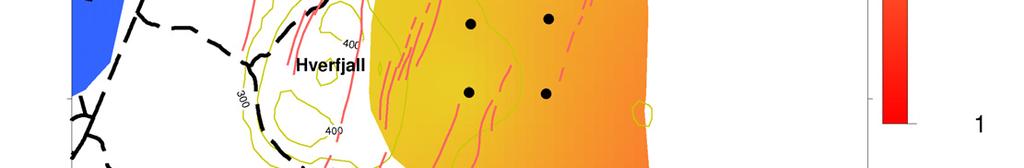
23 Report Sakindi In Figures 27 and 28, the Tipper strikes tangentially surround a body of limited area; this body is also shown by the corresponding induction arrows (Figure 29) which are facing away from the same area. A shown on the maps, this area is characterised by geothermal manifestations. Hydrothermal alteration indicates a subsurface conductive body; therefore, the Tipper strike and the induction arrows both indicate the existence of a conductive body in the same area. Finally, Figure 30 shows the Z-strike. FIGURE 27: Rose diagram of the electrical strike based on Tipper strike for the period 0.1 to 1 s. Blue (grey) dots are MT soundings where the H z components do not exist, grey lines are fractures, yellow (grey) areas are surface manifestations and dark red dashed lines are roads FIGURE 28: Rose diagram of the electrical strike based on the Tipper strike for the period 1 to 100 s; other symbols are explained in the caption of Figure 27

24 Sakindi 756 Report 30 FIGURE 29: Induction arrow diagram at 1s; other symbols are explained in the caption of Figure 27 FIGURE 30: Rose diagram of the electrical strike based on the Z-strike for the period 0.1 to 1 s; other symbols are explained in the caption of Figure 27

25 Report Sakindi 6. RESULTS OF RESISTIVITY MODELLING OF THE NÁMAFJALL AREA AND ITS GEOTHERMAL SIGNIFICANCE 6.1 Resistivity cross-sections and results from boreholes In this work, resistivity cross-sections were used to present the results of the inversion of TEM data and the joint inversion of TEM and MT data. The profiles are oriented N-S and W-E (see Figure 19) and an analysis was made by considering different depths. The program used to plot the resistivity crosssections from 1D inversion results is called TEMCROSS, developed at ÍSOR (Eysteinsson, 1998). The program is able to calculate the best line between the selected sites on a profile, then plot the isolines based on the 1D model generated for each sounding. The resistivities are contoured on a logarithmic scale; numbers at contour lines are resistivity values. A comparison between the resistivity structure and borehole data analysis was made in order to understand the subsurface geology of the Námafjall high-temperature geothermal field. Different investigations were carried out in order to acquire sufficient information from the Námafjall area. Gas geothermometers were applied to investigate the reservoir temperature: a maximum temperature above 300 C was observed east of Mt. Námafjall. Furthermore, high temperatures extend to the north and east sides of the main rifting zone (Gudmundsson, et al., 2010). Comparisons were made from data taken from the first nine boreholes, based on the cutting analysis and geophysical logs; the six last boreholes did not give clear fundamental results. Two logs from wells BJ- 11 and BJ-12 were selected to illustrate the general stratigraphy of the formations in the reservoir of Námafjall field. Sequences of lavas and hyaloclastites of basaltic composition characterize the reservoir formations, reflecting the environment during their formations. The hyaloclastites are accumulated volcanic glassy products that formed below the water table, most commonly in glaciers, which built up ridges and table-mountains. These features are dominant influences on the topography and indicate glacial periods. On the other hand, lava flows formed during interglacial time or shorter periods with ice-free conditions. The physical properties of lava and hyaloclastites vary a lot. Hyaloclastite is a heterogeneous material, with high porosity but variable permeability. The basaltic lavas are more homogeneous. The porosity is in the range of 5-15% and the permeability is rather high through the top and bottom scoria, as well as through the columnar jointing (Gudmundsson et al., 2010). The relative high quality of fracture fillings is a good indication of past or present permeability. A high abundance of the secondary mineral pyrite is evidence of good permeability. Pyrite is more abundant in the uppermost 1000 m where the variation in temperature ranges from 100 to 300 C, but its relative abundance where the temperature is above 300 C shows a good correlation with aquifers (Gudmundsson, et al., 2010). Knowledge on alteration minerals is important and Figure 31 shows some temperature dependent minerals in high-temperature areas in Iceland. From the analysis of alteration minerals for well BJ-11, it can be seen that the alteration FIGURE 31: Some temperature dependent minerals in high-temperature areas in Iceland (Gudmundsson et al., 2010)

26 Sakindi 758 Report 30 minerals are arranged in zones labelled with the name of the characterizing minerals (Figure 32). Beyond alteration zones, aquifers were found, located by circulation losses, pressure and temperature logs, as well as by tectonics. Therefore, from the analysis, a reasonable consistency between the measured temperature and alteration temperature could be concluded. Evidence of heating was observed and temperature-dependent minerals were identified in the Námafjall area. The maximum rise in temperature appeared in the northern part but, at 900 m depth, the isotherms were almost horizontal (Gudmundsson et al., 2010). FIGURE 32: Temperature according to alteration minerals in well BJ-11 (Gudmundsson et al., 2010) The two resistivity cross-sections N-S and W-E for Námafjall high-temperature geothermal field, are presented. Crosssection W-E is presented in Figures 33-35, with Figure 33 only based on TEM data while Figures 34 and 35 are based on joint inversion of TEM and MT data and reach down to 2500 m b.s.l. and m b.s.l., respectively. Figure 33 shows the conductive cap near the surface which correlates to the geothermal manifestations at the same place, which is the upflow zone FIGURE 33: Resistivity cross-section W-E based on TEM data

27 Report Sakindi FIGURE 34: Resistivity cross-section W-E, reaching down to 2500 m b.s.l. FIGURE 35: Resistivity cross-section W-E, reaching down to 10,000 m b.s.l. for the geothermal system; the resistivity is evaluated to be 1-5 Ωm at 300 m a.s.l. This conductive shallow zone seems to disappear around 250 m a.s.l. and another conductive zone starts from 200 m a.s.l. down to 100 m b.s.l., which correlates with smectite-zeolite alteration. The resistive core comes next, located between the shallower conductive zone, and a deeper one appearing at around 3000 m b.s.l. which could be linked to the heat source (Figures 34 and 35). Finally, Figure 36 shows good agreement between the resistivity layering and the alteration mineralogy as experienced in well BJ-15.

28 Sakindi 760 Report 30 FIGURE 36: Comparison between resistivity seen in cross-section W-E and borehole data Cross-section N-S (Figures 37-39) shows high resistivity close to the surface, Ωm, due to an unaltered formation. Below that comes the low-resistivity zone from 200 m a.s.l. (Figure 37). At a depth of around 3800 m b.s.l., a deep low-resistivity zone begins which may be connected to the heat source (Figure 39). 6.2 Resistivity maps (iso-maps) Iso-resistivity maps were compiled covering soundings from all four profiles found in the Námafjall area, using additional results from my fellow UNU-fellow, Uddin (2012), to gain a general idea of the resistivity distribution in the Námafjall high-temperature geothermal area. The program used is the TEMRESD program which can generate iso-resistivity maps at different elevations for 1D Occam models (Eysteinsson, 1998). In this report, iso-resistivity maps are presented from 300 m a.s.l. down to 20,000 m b.s.l., with the two uppermost iso-resistivity maps based on inversion of the TEM data and the deeper ones on the joint inversion of TEM and MT data. The iso-resistivity map at 300 m a.s.l. shows a low-resistivity zone in the central northeast part of the field delineating the surface activities of the geothermal field (Figure 40). The resistivity zone increases at sea level (Figure 41). This could be interpreted by the presence of high-temperature alteration minerals. This zone is surrounded by the high resistivity related to unaltered rocks. Similar scenario is seen at 3000 m b.s.l. (Figure 42). The high resistivity associated with the highresistivity core, where temperatures are expected to be >240 C is clearly seen and similarly at 5000 m b.s.l. (Figure 43). Changes are observed at deeper levels, 10,000 m b.s.l (Figure 44) as well as at 20,000 m b.s.l. (Figure 45). However, the resistive core seems to persist, but it was not possible to determine this clearly due to the low resolution of deeper layers.

29 Report Sakindi FIGURE 37: Resistivity cross-section N-S, based on TEM data FIGURE 38: Resistivity cross-section N-S, reaching down to 2500 m b.s.l.

30 Sakindi 762 Report 30 FIGURE 39: Resistivity cross-section N-S, reaching down to 10,000 m b.s.l. FIGURE 40: Námafjall, iso-resistivity map at 300 m a.s.l.; black dots are MT soundings, red (dark) lines are fractures, white colours show geothermal manifestations and black dashed lines are roads

31 Report Sakindi FIGURE 41: Námafjall, iso-resistivity map at sea level; symbols are explained in caption of Figure 40 FIGURE 42: Námafjall, iso-resistivity map at 3000 m b.s.l.; symbols are explained in caption of Figure 40

32 Sakindi 764 FIGURE 43: Námafjall, iso-resistivity map at 5000 m b.s.l.; symbols are explained in caption of Figure 40 FIGURE 44: Námafjall, iso-resistivity map at 10,000 m b.s.l.; symbols are explained in caption of Figure 40 Report 30

33 Report Sakindi FIGURE 45: Námafjall, iso-resistivity map at 20,000 m b.s.l.; symbols are explained in caption of Figure CONCLUSIONS AND RECOMMENDATIONS In this project the subsurface resistivity structure on two profiles across the Námafjall high-temperature geothermal field was analysed by using resistivity data and comparing them with alteration and temperature logs from boreholes. We can make the following conclusions based on the findings: The use of MT soundings for deep prospecting of geothermal systems in a volcanic area is most of the time accompanied by a static shift problem. It is necessary to correct this problem by applying TEM soundings and inverting the MT and TEM soundings jointly. This helps to avoid the high risk of ending up with misleading results that could otherwise occur. It is obvious that if the shifts are not properly treated, the interpretation could give false resistivity anomalies. Analysis of the electric strike is important in resistivity models. The conductive zone that lies above geothermal high-temperature systems has been shown to have a strong correlation with temperatures between C, dependent on the type of smectitezeolite alteration that occurs in this temperature range. The hotter parts of geothermal systems are characterised by higher resistivity. The low-resistivity cap reflects the smectite-zeolite zone. Smectite is a layered clay silicate with high cation-exchange capacity (CEC). A high-resistivity zone reflects a chlorite-epidote zone, more resistive as its ions are bound in a resistive crystal lattice and have low CEC.