Depths and focal mechanisms of crustal earthquakes in the central Andes determined from teleseismic waveform analysis and InSAR
|
|
|
- Horace Tyler
- 6 years ago
- Views:
Transcription
1 TECTONICS, VOL. 31,, doi: /2011tc002914, 2012 Depths and focal mechanisms of crustal earthquakes in the central Andes determined from teleseismic waveform analysis and InSAR S. Devlin, 1 B. L. Isacks, 2 M. E. Pritchard, 2 W. D. Barnhart, 2 and R. B. Lohman 2 Received 21 March 2011; revised 12 December 2011; accepted 21 December 2011; published 3 March [1] We investigate the depths of crustal earthquakes (<80 km depth) of the central Andes (5 S to 35 S) to constrain the relationship between earthquake locations and inferred faults. We assemble parameters from 138 moderate-sized (7.0 > Mw 5.5) earthquakes from the Global CMT catalog and previous work spanning For 38 well-recorded events, we use teleseismic P and SH waveforms to model the strike, dip, rake, focal depth, and source time function. We use InSAR observations of surface deformation from 9 earthquakes to compare inferred fault parameters with the waveform inversions and global catalogs to assess their accuracies. While the depths from the InSAR and waveform analyses generally agree within error, horizontal and depth errors in global catalogs are 10 to 50 km, as found elsewhere. As noted in previous work, the majority of crustal earthquakes occur in the Eastern Cordillera and foreland regions of the central Andes, although a few normal and strike-slip earthquakes occur beneath the Altiplano plateau and in the forearc in southern Peru and northernmost Chile. We propose a new interpretation of one of the basement thrusts (Shira Mountain, Peru) as a pop up block on the basis of our new earthquake depths. We confirm that earthquakes in the flat slab areas of Peru and Argentina are within the sometimes aseismic lower crust. Lower crustal earthquakes are globally found in all types of tectonic settings only when the thermal lithosphere is more than 80 km thick and the amount of recent shortening/extension is <30%. Citation: Devlin, S., B. L. Isacks, M. E. Pritchard, W. D. Barnhart, and R. B. Lohman (2012), Depths and focal mechanisms of crustal earthquakes in the central Andes determined from teleseismic waveform analysis and InSAR, Tectonics, 31,, doi: /2011tc Introduction [2] Earthquakes are one of the most widely observable indicators of ongoing lithospheric deformation, and their distribution within continents (particularly as a function of depth) provides insight into the location of active faults and the strength of the lithosphere. However, earthquake depths reported in standard global catalogs (e.g., ISC, International Seismological Centre; NEIC, USGS National Earthquake Information Center, Global CMT, centroid moment tensor) created by routine analysis of seismic waves, are not sufficiently accurate to be useful the errors in depth can reach 50 km, comparable to the depth of the continental crust [e.g., Maggi et al., 2000; Kagan, 2003]. Therefore, additional analyses using the surface reflected seismic phases (such as pp, sp, and ss) or ground deformation measurements (for example, from Interferometric Synthetic Aperture Radar or InSAR) are needed to constrain depths for continental earthquakes. In this paper we use both methods to systematically determine the depths of crustal earthquakes within 1 Office of New Reactors, U.S. Nuclear Regulatory Commission, Washington, D. C., USA. 2 Department of Earth and Atmospheric Sciences, Cornell University, Ithaca, New York, USA. Copyright 2012 by the American Geophysical Union /12/2011TC the central Andes for the first time since 1983 [Chinn and Isacks, 1983]. We use a standard waveform fitting method of the surface reflected phases to relocate the depths of 138 earthquakes between magnitudes 5.5 and 7.0 and the years 1944 and For 6 earthquakes we compare parameters inferred independently from both InSAR and seismic data. In addition, we use InSAR observations of 3 deformation patterns that may be caused by earthquakes in the global catalogs that are too small for detailed analysis with teleseismic waveforms. We combine our new locations and depths with topographic data, subsurface seismic imaging, and geologic interpretations to assess the potential origin structures for the earthquakes. 2. Study Area [3] The study area of the central Andes spans an area from 5 S to 35 S latitudes in western South America (Figure 1) and has great variability in crustal thickness and crustal seismicity. In the along-strike direction, there are three major segments of the subducted Nazca plate: the Peruvian and Chile-Argentine (a.k.a Pampean) flat-slab segments and the intervening segment where the subducted Nazca plate dips more steeply [e.g., Barazangi and Isacks, 1976; Jordan et al., 1983] (Figure 1). In the strike-perpendicular direction, there are major variations in crustal thickness and tectonics. From west to east, the regions are called (Figure 1): (1) the forearc, 1of33
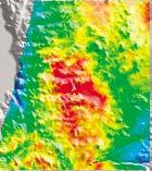
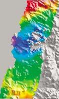
2 Figure 1. Generalized map of the central Andes. Gray contours show the depth (labeled in km) to the Wadati-Benioff zone of earthquakes within the subducting Nazca oceanic plate [Cahill and Isacks, 1992]. An approximate outline of the Altiplano-Puna, or central Andean, Plateau is the thick black line, which represents the 4 km contour line derived from SRTM (Shuttle Radar Topography Mission) topography. Black triangles illustrate recently active volcanic edifices [de Silva and Francis, 1991]. Shaded topography is from SRTM topography. between the trench and the volcanic arc (the zone of active volcanoes, or in the case of the flat slab segments, the zone of Miocene volcanism); (2) the hinterland, including the Altiplano-Puna plateau, the Eastern Cordilleras of Peru, Bolivia, and Argentina, and the Principal and Frontal Cordilleras of Argentina; and (3) the foreland, the region of youngest deformation, located east of the main cordillera, and bounded to the east by the undeformed craton. Examples of foreland regions are the Bolivian fold and thrust belt, and the Sierras Pampeanas of Argentina (Figure 1). [4] Previous comprehensive studies of seismicity in the central Andes [e.g., Chinn and Isacks, 1983; Jordan et al., 1983] have noted that the two most seismically active segments of the central Andes are the forelands of Argentina and Peru above the regions of flat-slab subduction. The crust of these regions is seismogenic from the surface to near Moho depth [e.g., Devlin, 2008], and the structural style is dominated by basement thrusts. Outside of these two foreland regions, the South American plate has previously appeared nearly aseismic with respect to earthquakes of magnitude Mw 5.5, appropriate for teleseismic recording. The apparent aseismic behavior of the Andean plateau contrasts with the seismicity of the Tibetan Plateau where earthquake focal mechanism orientations display patterns that strongly correlate with topography and deformational style [e.g., Andronicos et al., 2007; Langin, 2003]. [5] Earlier studies of seismicity within the central Andes [e.g., Alvarado and Beck, 2006; Alvarado et al., 2005, 2004; Alvarado and Ramos, 2011; Assumpção and Araujo, 1993; Dorbath et al., 1986; Kadinsky-Cade et al., 1985; Legrand et al., 2007; Regnier et al., 1992; Smalley and Isacks, 1990; Smalley et al., 1993; Stauder, 1975; Suárez et al., 1983] estimated earthquake source parameters in limited areas with locally recorded data, but not since Chinn and Isacks [1983] has there been a complete analysis and synthesis of continental seismicity for the entire central Andes. Since the majority of the earthquake record is limited to the last 50 years and large magnitude earthquake recurrence intervals are typically 100 years or more, continued monitoring of the seismologic activity reveals information about ongoing deformational provinces not previously observed. One goal of this study is to use 25 years of additional seismic data to assess whether the regions of the central Andes (particularly the Altiplano and Puna plateaus outside of Peru) are as aseismic as they appeared in earlier analysis and if earthquakes in the flat slab regions of Peru and Argentina occur in the lower continental crust that is generally assumed to be aseismic [e.g., Chen and Molnar, 1983]. Another goal is to compare the accurately located earthquake depths with new subsurface and topographic data sets to constrain the fault structures that might have caused the earthquakes. A final goal is to assess the accuracy of waveform depth determinations through comparison with independent observations of ground deformation from InSAR. 3. Methods 3.1. Earthquake Depth Determination [6] To determine earthquake depth distributions throughout the central Andes, three sources of data are considered: 1) previously published event parameters using local networks, 2) events recorded teleseismically by global seismograph stations for which earthquake source properties are constrained using waveform modeling or short-period depth phase identification, and 3) InSAR. The 138 earthquakes compiled for this study are listed in Table 1 and displayed in map view in Figure 2. Of these, 38 event parameters were constrained in this study, 48 have only Global Centroid Moment Tensor (CMT) solutions (a global earthquake catalog: and 52 are reported from previous studies using local seismometer arrays or teleseismic waveform analysis similar to that performed here (Table 1). These 2of33
3 Table 1. Central Andean Continental Earthquakes Date (mm/dd/yy) Time (hh:mm:ss) Location a c Nodal Plane 1 Nodal Plane 2 MT5 Solution Depth Reference Longitude Latitude Mw Strike Dip Rake Strike Dip Rake (km) Code b Mw Strike Dip Rake 01/15/44 23:49: AB06 06/11/52 00:31: AB06 05/12/59 09:46: CI83 05/18/63 05:33: CI83 11/13/65 17:59: CI83 04/25/67 10:36: AA93 06/19/68 08:13: CI S S75 06/20/68 02:38: CI S83 12/01/68 13:14: CI S83 07/18/69 23:17: CI83 07/24/69 02:59: CI S S75 10/01/69 05:05: CI S S75 02/14/70 11:17: CI S S75 10/15/71 10:33: S CI S75 03/20/72 07:33: CI S S75 09/26/72 21:05: CI83 11/03/73 14:17: CI83 11/19/73 11:19: CI83 07/01/74 16:51: CI83 05/15/76 21:55: CI S83 01/25/77 00:50: AA93 03/08/77 13:08: /02/77 14:47: /23/77 09:26: KC85 11/23/77 09:26: CI83 11/24/77 18:20: /28/77 04:19: /28/77 06:31: CI83 12/05/77 15:43: /06/77 17:05: CI83 12/10/77 07:11: /17/78 11:33: /21/78 00:28: /06/79 01:31: /30/79 18:59: /14/80 21:51: /09/80 08:17: /10/80 16:24: /18/81 17:05: /22/81 17:53: /19/82 04:27: /02/83 05:58: /03/84 04:10: /05/84 04:15: /26/85 03:07: /19/85 10:28: /22/85 14:02: /12/85 14:35: /11/86 05:04: /05/86 20:14: SHZ 05/09/86 16:24: /19/86 21:57: /11/86 22:06: /20/86 05:04: /13/87 20:08: of33
4 Table 1. (continued) Date (mm/dd/yy) Time (hh:mm:ss) Location a c Nodal Plane 1 Nodal Plane 2 MT5 Solution Depth Reference Longitude Latitude Mw Strike Dip Rake Strike Dip Rake (km) Code b Mw Strike Dip Rake 10/02/87 22:27: /15/87 22:00: /25/88 17:20: R92 03/16/89 17:12: SHZ 05/04/89 10:30: MT5 5.4 f 130 f 35 f 66 06/24/89 12:58: /30/90 02:34: MT /30/90 16:49: MT5 5.4 f 169 f 29 f /06/90 02:01: /04/91 15:23: MT /23/91 19:44: /02/93 15:44: MT5 5.3 f 293 f 61 f 4 10/02/93 00:06: /26/94 19:57: /12/95 03:35: MT /10/96 08:56: MT /06/96 09:18: /08/96 02:52: /17/97 22:14: /10/98 04:54: MT /19/98 04:21: MT /01/98 01:51: /06/98 03:56: MT /10/98 20:57: MT /12/98 23:49: MT5 SHZ f 5.8 f 313 f 44 f 47 05/22/98 04:49: MT /26/98 01:08: MT /29/98 11:23: MT5 5.4 f 84 f 81 f 2 10/04/98 13:41: MT5 5.7 f 188 f 28 f /25/98 03:54: SHZ 10/04/99 13:57: MT /25/99 18:19: MT /30/99 14:50: /30/00 05:31: /21/00 06:13: A05 12/25/00 00:49: A05 02/06/01 20:18: A05 02/09/01 01:11: A05 02/21/01 15:20: MT /15/01 11:06: A04 05/07/01 02:24: A05 05/10/01 02:24: A05 05/18/01 04:48: A05 05/18/01 07:12: A05 06/13/01 04:10: /20/01 01:26: A05 06/28/01 04:48: A05 06/29/01 22:33: MT5 SHZ f 5.4 f 320 f 36 f 65 07/04/01 12:09: MT /08/01 00:00: A05 07/24/01 05:00: MT5 SHZ /09/01 02:07: MT5 SHZ /09/01 06:45: /10/01 17:39: /12/01 00:16: SHZ 09/17/01 00:00: A05 10/12/01 04:21: /12/01 02:24: A05 11/24/01 00:00: A05 11/29/01 19:12: A05 12/04/01 05:57: MT5 SHZ f 5.8 f 239 f 73 f /05/01 00:00: A05 12/08/01 04:17: MT5 SHZ /14/01 00:00: A04 12/15/01 07:12: A05 12/18/01 07:12: A05 01/05/02 07:12: A05 01/19/02 19:12: A05 02/24/02 14:44: SHZ 03/10/02 12:00: A05 4of33
5 Table 1. (continued) Date (mm/dd/yy) Time (hh:mm:ss) Location a c Nodal Plane 1 Nodal Plane 2 MT5 Solution Depth Reference Longitude Latitude Mw Strike Dip Rake Strike Dip Rake (km) Code b Mw Strike Dip Rake 03/15/02 00:00: A05 04/17/02 04:48: A05 04/27/02 23:53: A05 05/04/02 12:51: /28/02 04:04: MT /02/02 20:21: MT /11/02 12:09: MT /04/02 21:03: /13/02 16:31: SHZ 05/03/05 19:11: MT /31/05 02:10: MT5 5.4 f 49 f 57 f /20/06 14:38: MT /24/07 19:13: MT5 f 5.5 f 103 f 40 f 91 a MT5 latitude and longitudes are taken from previously published local studies, the International Seismological Centre (ISC), or from the U.S. Geological Survey s National Earthquake Information Center (NEIC). b Reference codes: AB06, Alvarado and Beck [2006]; A05, Alvarado et al. [2005]; A04, Alvarado et al. [2004]; AA93, Assumpção and Araujo [1993]; CI83, Chinn and Isacks [1983]; KC85, Kadinsky-Cade et al. [1985]; MT5, from this study using P and SH waveform modeling; R92, Regnier et al. [1992]; SHZ, from this study using forward modeling of short-period depth phase arrival times; S75, Stauder [1975]; S83, Suárez et al. [1983]. Earthquakes with no reference code are from the Global CMT catalog no accurate depth is available for these events so no depth is listed. c Blank cells beneath the MT5 solution columns indicate that an MT5 solution is not available for that earthquake. When a number in the MT5 column is preceded by an f it means that this value was fixed in the inversion. studies should have errors in depth and focal mechanism similar or better to those presented here (see section 3.4). Some older events also have focal mechanisms from P wave first motion analysis and S wave polarization angles of teleseismic data. [7] Earthquakes with only CMT solutions but that are presumed to be crustal (e.g., less than or equal to regionally variable Moho depths of km) are included in Table 1. Their depths are left blank, because they lack accurate depth determination. The events are plotted on subsequent maps to help characterize the tectonics of the central Andes, but they are not considered during integration of subsurface structural data. [8] Below we give an outline of the methods used and error analysis. More complete details are available in Chapter 1 of work by Devlin [2008] Teleseismic P and SH Waveform Modeling [9] The theory behind the methods we use to determine earthquake source parameters is well-known and widely used. The relative time separation between direct P and SH wave arrivals and surface reflected phases, such as pp, sp, and ss, can be used to obtain accurate source depths, focal mechanisms, and source time functions for earthquakes with Mw 5.5 recorded at teleseismic distances (approximately 30 to 90 between station and receiver) by long-period or broadband seismographs [e.g., Helmberger, 1974; Langston and Helmberger, 1975; Nabelek, 1984; Lay and Wallace, 1995]. The effects of the velocity structure, attenuation response of the earth, and the impulse response of the seismograph are convolved with the effects of the source properties to determine the incoming waveform properties at the receiving seismograph. The synthetic seismograms are compared with the observed seismograms from stations at various distances and azimuths and the input parameters are iteratively changed until the synthetic seismograms reasonably match the observed seismograms. Waveform comparisons are made visually and by a method of minimization of the difference between the observed and synthetic waveforms (discussed in Section 3.4). [10] Of the 38 events with depths determined in this study, 32 earthquake solutions included P and SH teleseismic waveform modeling (labeled MT5 in Table 1 References column). The procedure involved downloading broadband seismograms from the Global Digital Seismograph Network (GDSN) and changing the frequency response to that of a WWSSN s long-period instrument using a deconvolution procedure. For this range of periods, seismic waves are relatively insensitive to complexities in local velocity structure, and the earthquakes considered here are modeled as point sources. [11] We use the MT5 program (P. Zwick et al., MT5, IASPEI Software Library, , hereinafter Zwick et al., 1994) developed from the algorithms of McCaffrey and Abers [1988] and McCaffrey et al. [1991] to forward model or invert P and SH waveform data. When the data quality is high (good azimuthal coverage of stations and strong signal-to-noise ratio), we invert for the source time function, moment, strike, dip, rake and depth. Global catalog epicentral locations from the ISC and NEIC catalogs are used for the seismic analysis (Table 1), although it is known that these locations can differ from InSAR locations by up to km (Figure 3) with a global median value of about 10 km [Weston et al., 2011]. The MT5 program does not allow for inversion of the latitude and longitude of the earthquake and previous work has also assumed the horizontal locations from the global catalogs [e.g., Molnar and Lyon-Caen, 1989; Maggi et al., 2000]. The impact of these epicentral location errors will be discussed in section 4 while the horizontal location could impact the tectonic interpretation, it does not seem to have a large effect upon the inferred depth (R. McCaffrey and G. Abers, personal communication, 2011). We constrain the source to be a pure double-couple with the source time function represented by a single isosceles triangle (after an initial set 5of33
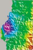
![the strongest initial phase arrivals (P, pp, sp, S, ss) this is a valid approximation for the first 25 s of the seismogram for the small earthquakes we are studying [Helmberger and Burdick, 1979].](/docs-images/71/65514097/images/6-0.jpg "[13] When data quality, quantity, or azimuthal distribution is poor, a full MT5 inversion solution can be difficult, so we use two alternatives to a full solution inversion to constrain all source")
6 the strongest initial phase arrivals (P, pp, sp, S, ss) this is a valid approximation for the first 25 s of the seismogram for the small earthquakes we are studying [Helmberger and Burdick, 1979]. [13] When data quality, quantity, or azimuthal distribution is poor, a full MT5 inversion solution can be difficult, so we use two alternatives to a full solution inversion to constrain all source parameters, or at least source depth. One alternative holds moment, strike, dip, and rake fixed to that of the seed solution and only inverts for a best fit depth. The second alternative is used when depth solutions are available using short period vertical component waveforms (SHZ, described in section 3.3). Source depth is held fixed to the SHZ solution and inversion for best fit focal mechanism and moment is then carried out. For each earthquake, we make plots of the waveform inversion solution and sensitivity to different source parameters (Section 3.4). Figure 2. Continental seismicity of the central Andes. Base map is 90 m SRTM topography. Earthquake focal mechanism solutions (Tables 1 and 4) are represented in lower hemispheric projections, where dark quadrants contain compressional motions and the T axis. Accurate event depths are labeled in red. Black points are the four subduction zone earthquake sequences (including six earthquakes total) that are compared to InSAR. Other symbols as in Figure 1. of inversions with multiple triangles in the source time function [Devlin, 2008]). [12] We model P, pp and sp phases on vertical component seismograms in the epicentral distance range 30 to 90, and S and ss phases on transverse components in the range 30 to 75. We correct waveform amplitudes for geometrical spreading and for anelastic attenuation using a Futterman Q operator with a value t* of 1.0 s for P and 4.0 s for SH waves. For local source structure, we use a simple half-space model with velocities VP = 6.5 km/s, VS = 3.7 km/s and density r = 2800 kg/m3. For global travel times we use the IASPEI 91 velocity model [Kennett and Engdahl, 1991]. We model only 3.3. Short-Period Vertical Waveform (SHZ) Depth Determination [14] To provide an additional constraint on focal depth, we use depth phases (the surface reflections pp and sp) from short-period, vertical component, teleseismic records for some events. While surface reflected phase identification can be difficult without waveform modeling on broadband or long-period records (e.g., using the MT5 algorithm of Section 3.2), higher frequency short- period waveforms can sometimes reveal differential travel times of pp-p and sp-p, thereby allowing a depth estimate to be made. Where shortperiod and long-period records are both available, combining these two methods can provide additional robustness to depth determination. For example, for smaller magnitude events, where most of the teleseismic long-period signals are too small for modeling, short-period depth phase identification may provide the only depth estimate available. In practice, we first pick pp-p and sp-p times on short period waveform records. Then we test a series of forward models (varying the source depth) using the half-space velocity structure from Section 3.2 and the TTIMES program [Kennett et al., 1995; Montagner and Kennett, 1996] (Which uses the IASPEI 91 velocity model) to calculate the estimated phase arrival times. The differential travel times between pp-p and sp-p provided by TTIMES is then compared to the times picked on the seismic record. The best fitting depth reported by TTIMES is used as the SHZ depth solution in Table Seismic Error Analysis [15] Previous analyses have shown that uncertainties of the inferred fault parameters calculated from teleseismic waveform inversion programs like MT5 are: strike 10, dip 5, rake 10, and depth 5 km [e.g., Mitra et al., 2005; Stein and Kroeger, 1980]. We think our uncertainties on fault parameters are similar. In this section, we consider in turn how various parameters that are input to and output from the MT5 inversion affect the inferences of the fault parameters, especially depth: the velocity structure, syntheticto-observed waveform misfit, initial estimate of focal mechanism, and trade off between depth and source time function. [16] Chinn [1982] found that if model seismic velocities are within 10% of the true bulk crustal velocity, then errors in depth are similarly 10%. The velocity model used in this study is an average of models used in previous earthquake 6 of 33

7 Figure 3 7of33
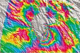
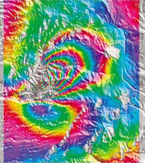
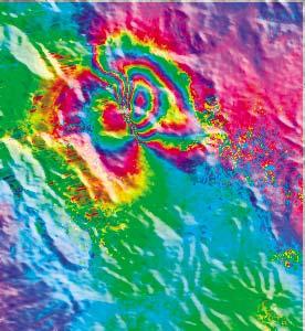
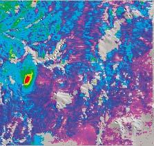
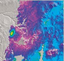
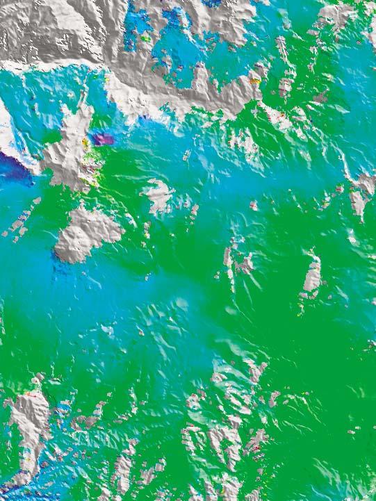
8 location and seismic imaging studies in the limited parts of the central Andes with available data [e.g., Alvarado et al., 2005; Chinn and Isacks, 1983]. Our model meets the criteria of agreement (10%) with bulk crustal velocities used in local network seismic studies spanning the forearc to the backarc [e.g., James and Snoke, 1994; Smalley and Isacks, 1990; Legrand et al., 2007]. [17] The MT5 algorithm minimizes the weighted squares of residuals between the relative amplitudes of the synthetic and observed seismograms summed over all the stations to obtain the best fit solution. It adjusts the event source time function, seismic moment, focal mechanism orientation, and depth to minimize the misfit, although for some earthquakes, as mentioned above, a few parameters were held fixed during the inversion and are listed as such in Table 1. In Figure 4, we show waveforms of an example event (4/4/1991) and Figure 5 is a plot of earthquake depth versus a misfit parameter output by MT5 called R/D% illustrating the sensitivity to source depth. The R/D% is a weighted and normalized value that shows as a percentage how much the variance of the original data is reduced by the model (Zwick et al., 1994). The minimum misfit is a local, not a global minimum, because the misfit depends on how the source time function is parameterized, among other variables. [18] However, residual statistics of teleseismic waveform inversions (like R/D%) have been shown to underestimate the true uncertainties associated with source parameters [McCaffrey and Nabelek, 1987]. Therefore, as a check on the quantitative estimate of the model with the lowest misfit, we visually inspect the waveforms to determine within what parameter window the synthetics fit the observed waveforms as suggested by others [e.g., Emmerson et al., 2006; Maggi et al., 2000; McCaffrey and Nabelek, 1987; Molnar and Lyon-Caen, 1989]. Figure 6 shows a sample sensitivity analysis for the same earthquake (4/4/1991) featured in Figures 4 and 5. Sensitivity analysis plots illustrate the window of solution parameters, in particular the range of depths, which fit the observed waveforms. Figure 6 shows five of twenty-seven waveforms used in the inversion and five different event parameters to compare how the different parameters affect the fit between synthetics and the observed waveforms. The line in Figure 6a is the best fit inversion solution and lines in Figures 6b and 6c illustrate the depth range over which the synthetic waveforms match the data. For this particular event, the waveform fit is consistent for a depth range of 3 km, which is illustrated by the good, but deteriorating, synthetic-to-observed waveform fit of the solution for 26 km depth (Figure 6b) and for 32 km depth (Figure 6c). Also shown in Figure 6 is how well the Global CMT (Figure 6d) and the NEIC (Figure 6e) focal mechanism solutions fit the observed waveforms. The complete set of plots like Figures 4 and 6 for each earthquake is contained in Appendix A of work by Devlin [2008]. [19] We typically begin the MT5 inversion with a starting focal mechanism from the Global CMT [e.g., Dziewonski et al., 1981] or NEIC catalogs, followed by an inversion using an iterative approach for the focal mechanism solution that best fits the P and SH waveform data. Typically, CMT focal mechanism orientation errors vary from 5 to 20 depending on the quality of the solution [e.g., Kagan, 2003]. Usually, our inverted solutions from MT5 differed from the initial CMT or NEIC by less than 10 and never did the MT5 solution change mechanism type from that of the CMT solution (e.g., from a thrust to a normal or strike-slip mechanism). In a few cases, the MT5 focal mechanism solution did deviate from the CMT solution by as much as 27, as defined by the change in null axis orientation. [20] On certain waveforms, the depth and source time function parameters can be coupled [Christensen and Ruff, 1985], which adds uncertainty to solution determination. Although we minimized this trade-off by using seismograms from a variety of distances and azimuths, there remain some events where only a few observed seismograms were available for matching and azimuthal distribution of recording stations is poor. For most of the small earthquakes studied here, we think that the single triangular source time function is a fair representation of the event based on that fact that we compare the single triangle result to one with more degrees of freedom (see Devlin [2008] for details). As we discuss in section 4.1, it is critical to use the proper length for the source time function InSAR [21] Interferometric synthetic aperture radar (InSAR) is a technique that can be used to generate maps of surface deformation caused by earthquakes and can be used as an independent estimate of earthquake fault parameters [e.g., Bürgmann et al., 2000; Rosen et al., 2000]. We can then compare the solutions to the teleseismic waveform results. We analyze InSAR data from nine earthquakes (Tables 2, 3, and 4 and Figure 3) six of these earthquakes are studied with both InSAR and the teleseismic data and three are studied only with InSAR because they are too small for waveform analysis at teleseismic distances. Seven of these earthquakes have been the subject of previous work [Pritchard, 2003; Funning et al., 2005; Pritchard et al., 2006; Holtkamp et al., 2011] while two events are analyzed here for the first time (Chile earthquakes in 1995 and 2001). Four earthquakes are assumed to be located along the Chile subduction zone between 25 S and 30 S although these earthquakes are not crustal, they help to assess the ability of the teleseismic data to resolve fault depth within our study area. For the four subduction zone earthquakes, a surface water layer is included during the teleseismic waveform inversion. While subduction zone earthquake hypocenters can be systematically shifted for several reasons [e.g., Figure 3. Interferograms used in this study to constrain earthquake parameters. Each plot has a different color scale so that the earthquake deformation would be most obvious. Table 5 lists the dates of each interferogram. Stars with black borders show hypocenter locations from global catalogs (NEIC unless otherwise labeled.) Stars with red borders are those taken from a global catalog for waveform analysis. Focal mechanisms are from the Global CMT catalog unless otherwise noted. (a d) Subduction zone earthquakes, with fault parameters shown in Table 2. (e h) Earthquakes with magnitudes too small for teleseismic waveform modeling and which are only studied with InSAR (Table 4). (i j) Shallow crustal earthquakes studied with both InSAR and waveform modeling (Table 3). Stars with blue outlines show the center of the InSAR-derived fault plane. 8of33
9 Figure 4 9of33
10 Figure 5. R/D% versus depth plot for the inversion example shown in Figure 4. Each data point represents an inversion where the depth and source time function were held fixed. Filled circles are inversions where focal mechanism orientation was permitted to vary The square and cross data points represent forward modeling solutions of P and SH waveforms where the focal mechanism and depth solutions were held fixed for the NEIC and CMT reported solutions, respectively. Syracuse and Abers, 2009], the majority of these earthquakes do not seem to be biased in this way [Engdahl et al., 1998]. We attempted to study two earthquakes in Ambato and Salta, Argentina (on 7 Sep and 27 Feb. 2010, respectively) (Table 5), but the interferometric coherence was too low to observe the events because of the vegetation in the area. [22] InSAR data are from the ERS-1, ERS-2 and Envisat satellites of the European Space Agency (with a C-band radar, 5.6 cm wavelength) (Table 5). While the data quality from the C-band radars in the Altiplano-Puna and forearc regions is high [e.g., Pritchard and Simons, 2004] because of the generally arid climate, interferograms are of lower quality in the Eastern Cordillera [e.g., Funning et al., 2005] and unusable in the foreland region when the available interferograms span multiple years. Observations of individual earthquakes include several weeks to months of potential preseismic and post-seismic deformation because of infrequent satellite data acquisitions, but we neglect these sources of deformation since we assume that they are small for these shallow, moderate earthquakes for example the seismic moment of the post-seismic deformation following the crustal 2003 Mw 6.5 San Simeon, California was 14% of the co-seismic moment [e.g., Johanson and Bürgmann, 2010]. [23] We use the ROI_PAC software for InSAR processing [Rosen et al., 2004]. The number of data points in the interferograms was reduced from millions to thousands by subsampling a spatially compressed interferogram with a density of points determined by a data resolution matrix [Lohman and Simons, 2005b]. This resampling method requires that a starting model be chosen, but the resampling does not significantly depend on the model chosen as long as the strike and dip are within about 30 degrees (which is well within the accuracy of the global CMT solution). Interferograms were Figure 4. Sample waveform inversion solution plot from MT5 program. The header contains the date of the seismic event on the first line and the results of the inversion (strike, dip, rake, depth in km, and seismic moment in N-m) on the second. The letter F is placed in front of the strike or depth solution parameter when the focal mechanism or depth, respectively, has been held fixed. The upper sphere shows the P- wave radiation pattern and the lower sphere that for SH. Both are lower hemisphere projections. The station code by each waveform is accompanied by a letter corresponding to its position in the focal sphere. These are ordered clockwise by azimuth. The solid lines are the observed waveforms and the dashed lines are the synthetic waveforms. The inversion window is marked by the solid bars at either end of the waveforms. P and T axes within the sphere are represented by solid and open circles, respectively. The source time function (STF) is shown below the P focal sphere, with the waveform timescale below it. Timescales are in seconds (s). 10 of 33
11 Figure 6. Sample sensitivity analysis for the event shown in Figures 4 and 5. Each row shows a different waveform inversion solution. The title line shows the event date (yyyy/mm/dd), ISC reported origin time (hh:mm:ss.ss), ISC reported location (latitude, longitude), and CMT reported magnitude. When ISC origin time and location are unavailable, the CMT time and location are listed. P and SH focal spheres are shown in the first column. Strike, dip, rake, depth (km), and seismic moment (N-m) are labeled above the focal spheres. The source time function is shown above the waveform timescale in the second column followed by the observed and synthetic waveforms in the subsequent columns. Timescales are in seconds (s). Waveform display convention is the same as that in the waveform inversion solution plots (e.g., Figure 4) and here the station code and phase type (shown in parentheses) are located above the waveforms. (a) The MT5 minimum misfit solution. (b) The shallow depth bound of the waveform inversion and (c) the deeper bound, such that the synthetic data fit the observe fairly well between 23 and 32 km depth and deteriorate thereafter, so according to waveform fit this event occurred at a depth of 29 3km. (d) How well the CMT solution (focal mechanism, depth, and moment) fit the observed data and (e) that for the NEIC solution (focal mechanism, depth, and moment). In contrast to lines in Figures 6a, 6b, and 6c, lines in Figures 6d and 6e test how well catalog solutions fit the data and verify that deviations from catalog solutions are necessary to fit the waveforms. power-spectrum filtered using the algorithm of Goldstein and Werner [1998] and unwrapped using the branch-cut algorithm of Goldstein et al. [1988] that is part of the ROI_PAC software. Unwrapping was done at different pixel resolutions, about 180 m/pixel for the Mw < 6 earthquakes and between 360 and 1440 m/pixel when Mw > 6 because the lower spatial resolution was sufficient to resolve the deformation from these larger and deeper earthquakes. Digital elevation models from the Shuttle Radar Topography Mission with about 90 m pixel spacing are used to remove the topographic signature from the InSAR phase [Farr et al., 2007]. Noisy areas were masked out using a phase variance threshold and additional unwrapping errors were manually removed before modeling. [24] We do a formal inversion to optimize earthquake parameters to match the observed interferograms. We use the Neighborhood Algorithm [Sambridge, 1998] for all earthquakes except for the two small and deep earthquakes (1993 and 1996 Chile) studied by Pritchard et al. [2006]. In addition to inverting for fault geometry, we solve for the absolute value of the phase InSAR measurements are relative and not absolute, so we must account for the fact that zero phase in the interferogram might not correspond to zero ground deformation. We also solve for spatial variations in the 11 of 33
12 Table 2. Subduction Zone Earthquakes Studied Using InSAR for Comparison With the Waveform Methods a Method Longitude (deg) Latitude (deg) 1993/07/11 Mw 6.8 CMT n/a n/a Pritchard et al. [2006] f f f MT5 (this study) n/a n/a 1995 events near La Serena, Chile Depth (km) Mw Strike (deg) Dip (deg) Rake (deg) Length (km) CMT 1995/11/ n/a n/a InSAR [Devlin, 2008] InSAR (this study) e e f6 f25 f MT5 (this study) 1995/11/ n/a n/a MT5 (this study) 1995/10/ n/a n/a 1996/04/19 Mw 6.7 CMT n/a n/a Pritchard et al. [2006] f f f MT5 (this study) n/a n/a 2006/04/30 seismic swarm on subduction zone near Copiapó, Chile CMT 21:41: n/a n/a CMT 19:17: n/a n/a InSAR [Devlin, 2008] InSAR [Holtkamp et al., 2011] b 21 b MT5 (this study) 19:17: n/a n/a MT5 (this study) 21:41: n/a n/a a When a number is preceded by an f it means that this value was fixed in the inversion. Error bounds from this study correspond to one standard deviation from the Monte Carlo analysis of the impact of atmospheric errors on the interferograms. b These parameters were fixed in the preferred inversion, see Holtkamp et al. [2011] for details. Width (km) InSAR phase to correct for errors in the satellite orbital parameters and long-wavelength deformation patterns (e.g., inter-seismic deformation from the subduction zone earthquake cycle). For most of the small earthquakes, linear ramps are removed, but quadratic ramps were used for the earthquakes that we include here from Pritchard et al. [2006], because the longer interferograms used require quadratic ramps [e.g., Fournier et al., 2011]. InSAR fault models are calculated in an elastic half-space [Okada, 1985], (just like the P and SH waveform modeling analysis), so any difference in depth between the InSAR and waveform modeling is not due to differences in the elastic media used InSAR Statistical Depth Analysis [25] To estimate error bounds on the InSAR-derived fault parameters, we apply Monte Carlo error analyses to five of the earthquakes (1994 Peru, 1995 Chile, 1998 Bolivia, 2001 Chile, 2005 Peru; Tables 3 and 4). This methodology allows us to estimate errors associated with correlated atmospheric noise in individual interferograms but does not account for errors induced by our assumption of a homogenous elastic half-space. Using the Neighborhood Algorithm [Sambridge, 1998], we invert for a best fitting single finite fault patch and slip magnitude from a single resampled interferogram for each event. Data quality among the interferograms was not uniform and slightly different strategies were used. For earthquakes that were offshore or too small in magnitude we had to fix some of the model parameters (see Tables 2 4 for which parameters were fixed). When inverting for the best fit model for the 1998 Bolivia and 2001 Chile events, we allow all aspects of the fault model to vary, including orientation, geometry, and location. We use the best fit fault model to derive 1000 synthetic data sets and add correlated noise with length scales varying from 5 km to 65 km as determined from estimating the data covariance matrix from the original interferogram [Lohman and Simons, 2005b]. We then invert each synthetic data set allowing for a variable fault geometry and location. In each inversion of the synthetic data, we allow location, orientation, area, and depth to vary. 4. Results 4.1. Comparison of InSAR and Seismic Depth Estimates [26] For each earthquake, Tables 2 4 list earthquake solution parameters reported by the Global CMT catalog, previous studies, InSAR analysis, and results from P and SH waveform inversion (only available for Tables 2 and 3). [27] Interferograms of the four subduction zone earthquakes are shown in Figure 3, and while the NEIC and ISC Table 3. South American Crustal Earthquakes Studied Using InSAR and With the Waveform Methods a 1998/5/22 Aiquile, Bolivia Mw /7/24 Aroma, Chile Mw 6.3 Method Longitude (deg) Latitude (deg) Depth (km) Mw Strike (deg) Dip (deg) Rake (deg) Length (km) CMT n/a n/a InSAR [Devlin, 2008] InSAR (this study) e e Funning et al. [2005] MT5 (this study) n/a n/a CMT n/a n/a Legrand et al. [2007] InSAR (this study) e e f InSAR [Devlin, 2008] MT5 (this study) n/a n/a a See Table 2 footnotes for further information. Width (km) 12 of 33
13 Table 4. South American Crustal Earthquakes Studied Only With InSAR a 1994/12/26 Peru Mw /7/25 and 1997/7/27 Chile Mw seismic swarm near Ticsani, Peru Method Longitude (deg) Latitude (deg) Depth (km) Mw Strike (deg) Dip (deg) Rake (deg) Length (km) CMT n/a n/a ISC (mb) n/a n/a n/a n/a n/a NEIC (mb) n/a n/a n/a n/a n/a Pritchard [2003] n/a n/a InSAR (this study) f1 f1 NEIC 7/25/ (mb) n/a n/a n/a n/a n/a ISC 7/25/ (mb) n/a n/a n/a n/a n/a NEIC 7/27/ (mb) n/a n/a n/a n/a n/a ISC 7/27/ (mb) n/a n/a n/a n/a n/a Pritchard [2003] n/a n/a CMT 8/3/ n/a n/a CMT 10/1/ n/a n/a CMT 10/2/ n/a n/a ISC 10/1/ (mb) n/a n/a n/a n/a n/a Holtkamp et al. [2011] InSAR (this study) e e a See Table 2 footnotes for further details. Width (km) locations for all the events are near the areas of deformation, three of these earthquakes show Global CMT locations that are all shifted west of the deformation by 40 km [Pritchard et al., 2006]. Of the four subduction zone earthquakes, two of the events are likely to have a significant component of surface deformation offshore where it cannot be measured by InSAR (earthquake sequences in 1995 and 2006), while the two events onshore (earthquakes in 1993 and 1996) are significantly deeper (50 km as opposed to 25 km depth for the 1995 and 2006 events) and are at the limit of detectability of InSAR (Figure 3). Thus, all InSAR inversions for the subduction zone earthquakes must be constrained in some way to reach a satisfactory solution. The 1993 and 1996 earthquakes had their depths fixed. For the 1995 Chile event, we fix the fault orientation to the MT5 result (Table 2) and allow fault location, area, and depth to vary. We then generate 500 synthetic data sets for each of the best fitting single fault patch models, add correlated noise as before and invert using the Neighborhood Algorithm. Our iterative approach for the 2006 earthquake sequence is described by Holtkamp et al. [2011]. We assume that the earthquakes near the subduction zone megathrust occur on the low angle, east-dipping nodal plane (the plane most consistent with the subduction zone plate interface). [28] The interferograms spanning the earthquake sequences in 1995 and 2006 include several earthquakes with Mw > 5.5, but the ground deformation is dominated by the largest earthquake in each sequence (about Mw 6.7). The InSAR inversion includes all of these earthquakes as a single event, while we perform separate MT5 inversions for the largest earthquakes in each sequence (Table 2). All of the InSAR and MT5 inferred depth parameters are within the estimated error bounds from section 3.4 (5 km) of each other. [29] For our study area, we can only directly compare InSAR and teleseismic waveform inversions of all model parameters (depth, strike, dip, rake, and moment) for the 2001 Chile and 1998 Bolivia events (Table 3). For the 2001 Chile earthquake, the depths determined by InSAR, teleseismic analysis and previous work are in agreement given the uncertainties and the finite size of this Mw earthquake. As can be seen in Figure 7b, our best fit InSAR finite slip fault model does not account for all structure in the deformation field, suggesting that we do not optimally fit the data by using a single finite fault source and that distributed slip model is required by the data (as found by Funning et al. [2005] for the 1998 Bolivia event) but beyond the scope of this work. [30] The depths determined from InSAR and teleseismic waveform analysis for the Mw , Bolivia earthquake do not agree well (depths of 11 5 km for teleseismic and km for InSAR), but the error bars quoted are likely too small when the finite size and source time function for this relatively large event are considered. The depths of both the MT5 and InSAR solutions are referenced to the same datum (the local average elevation), which is about 3 km in this area. The fit to the teleseismic waveforms is nearly Table 5. InSAR Data Used in This Study Earthquake Name Earthquake Date Satellite Track Date 1 Date 2 Perpendicular Baseline (m) Peru 12/26/1994 ERS /7/1995 7/7/ Chile 11/1/1995 ERS 325 5/21/1996 5/24/ Chile 7/25/1997? ERS /24/2000 5/18/ ERS 53 8/6/1999 3/14/ Aquile, Bolivia 5/22/1998 ERS 239 7/30/1998 4/11/ Aroma, Chile 7/24/2001 ERS 96 12/10/2007 5/8/ Ambato, Argentina a 9/7/2004 Envisat 196 2/20/ /8/ Envisat 196 7/14/ /8/ Salta, Argentina a 2/27/2010 Envisat 196 2/20/2006 4/5/ a No deformation observed because earthquake area was incoherent. 13 of 33
14 Figure 7. Example of modeled interferogram, residual between data and model and error bounds on the inversion for source depth for the 2001 Mw. 6.5 Aroma, Chile earthquake (interferogram shown in Figure 3). (a) Best fit model of the line-of-sight deformation using model parameters from Table 4. Rectangle shows the location of the fault plane. (b) Residual between model from Figure 7a with observed interferogram. (c f) Histograms of model parameters (depth, strike, dip and rake) derived from 1000 inversions of the model shown in Figure 7a with artificial correlated noise with a length scale calculated from the data. Depth is to the center of the inverted fault shown divided into 20 bins. Vertical gray bars show 1 sigma error bounds. identical for depths between 5 and 13 km (Figure 8) when we change the source time function duration or number of subevents allowed. The 11 km depth was chosen for Table 1 because it provides the lowest R/D% misfit parameter when only a single isosceles triangle source time function is allowed (12 s). A depth of 5 km has the overall lowest misfit of all the models we examined (with a source time function with 7 triangles, each with 4 s duration; Figure 8), but the improvement to the fit may not be statistically significant given the number of additional free parameters. The finite size of this Mw 6.6 earthquake (fault length and width of order 10 to 20 km) is resolvable by the InSAR data the distributed slip model of Funning et al. [2005] places most slip between 5 to 7 km (Figure 9 and Table 4). The MT5 model assumes that the entire fault ruptures as a point source, and does not consider the finite size of the rupture. Considering the filtering applied to the teleseismic data (only including periods of 15 to 100 s) this point source approximation is reasonable because the seismic wavelength of 100s of km that is greater than the fault dimensions. [31] Figure 3 and Table 4 include three areas of deformation that we think are plausibly related to earthquakes, but that have Mw < 5.5 and are too small for teleseismic analysis. These potential earthquakes are included because they provide additional constraints on the accuracies of the global catalogs and their tectonic setting. The deformation pattern most likely associated with an earthquake sequence near Ticsani volcano in July to October, 2005 (Figure 3f) and described in more detail by Holtkamp et al. [2011]. The total moment (from the Global CMT catalog, about equivalent to a Mw 5.6) of the three largest earthquakes appears to explain all of the observed deformation (2005/8/3 Mw = 4.9; 10/1/ 2005 Mw 5.3; 2005/10/2 Mw = 5.1), but the CMT locations for these events are km away from the actual deformation pattern (which is not surprising considering the global analysis of Weston et al. [2011]). The normal faulting mechanism from the InSAR and CMT results is broadly similar. [32] Figures 3g and 3h shows an elliptically shaped deformation pattern (about 4 cm LOS, mostly due to uplift) that cannot be obviously related to any hydrothermal activity or anthropogenic sources of deformation (wells, mines, etc.), and we suggest that it might be due to a small, shallow, earthquake [Pritchard, 2003]. This pattern has been observed in independent interferograms, and we constrain the deformation to have occurred between 5/23/ /10/1997. Figures 3g and 3h show the epicenters for the closest earthquakes in the ISC and NEIC catalogs to the deformation pattern during the time period when deformation could have occurred. The epicenters of the earthquakes on 7/27/1997 and 7/25/1997 are closest to the deformation (with Mb 4.3 5), but according to the seismic data, both earthquakes have depths exceeding 20 km, with many solutions favoring depths between 40 and 50 km. The inversion of Pritchard [2003] has a depth of 3.5 km with a thrust mechanism, which is tectonically reasonable for this area of topographic expression of compression, but there are no other focal mechanisms in this area for comparison (Figure 2). [33] A region of localized subsidence (about 3 cm LOS maximum deformation) can be seen in southern Peru to the 14 of 33
15 Figure 8. Waveform inversion solution for the 1998 Aiquile, Bolivia earthquake. Figure conventions are those described in Figures 4 and 6. We show results with source time functions of different lengths (using a single triangle) and multiple triangles as well. The bottom line of the sensitivity analysis plot tests the waveform fit of the solution from Figure 9 and listed in Table 4 as InSAR (this study). Figure 9. Example of modeled interferogram, residual between data and model and error bounds on the inversion for source depth for the 1998 Mw. 6.5 Aiquile, Bolivia earthquake. Interferogram is shown in Figure 3 two frames of InSAR data ( ) were used instead of the one frame (3962) used by Funning et al. [2005]. (a) Best fit model of the line-of-sight deformation using model parameters from Table 4. Rectangle shows the location of the fault plane. (b) Residual between model from Figure 9a with observed interferogram. (c f) Histograms of model parameters (depth, strike, dip and rake) derived from 1000 inversions of the model shown in Figure 9a with artificial correlated noise with a length scale calculated from the data. Depth is to the center of the inverted fault shown divided into 20 bins. Vertical gray bars show 1 sigma error bounds. 15 of 33
16 N-NE of Hualca Hualca volcano in multiple interferograms [Pritchard, 2003] (Figure 3e), and we suspect the deformation is due to an earthquake in the common time period (8/24/ /31/1993). Figure 3e shows the cataloged earthquakes closest to the deformation during the time period, with the earthquake on 12/26/1994 being the most plausible candidate, given that this is the closest location in the ISC catalog and our inversion for the source gives a Mw 4.9, close to the catalog moments (Mb 5), and a mechanism similar to the Harvard CMT solution. However, our location is km from the catalog locations and our depth is only 1.4 km, compared to km in the catalog. The offset between the InSAR solution and the global catalog is within the range of discrepancies between InSAR and seismic hypocenters observed elsewhere [e.g., Lohman and Simons, 2005a; Weston et al., 2011]. Although the offsets of 45 km horizontal and 44 km in depth would be at the upper edge of the range, this might not be surprising considering the small size of this earthquake might be harder for the global catalogs to locate. Alternatively, the residual could be related to fumarolic or other volcanic activity, but since this type of deformation is not observed in other time periods, we think the earthquake explanation is most plausible. [34] In summary, for the six earthquakes with both teleseismic and InSAR data, we find that the inferred depths agree within uncertainty, although we make two caveats. The depths of three of the four subduction zone earthquakes had the depths in the InSAR inversion fixed to the assumed depth of the megathrust in their respective locations (probably known within about 10 km) this still confirms that the MT5 depth is consistent with the subduction interface. For the 1998 Bolivia earthquake, the InSAR and waveform data are consistent with a 6 7 km depth for this earthquake, when the trade-off between source time function and depth is considered [Christensen and Ruff, 1985]. We did not use the MT5 software to adjust the horizontal location of the earthquakes, but the uncertainty in this location is important for the tectonic interpretations in the next section. For five of the six earthquakes with Mw > 5.5, the InSAR horizontal locations are within 10 km of the ISC and NEIC global catalogs (mislocation of the global CMT locations are larger as expected [Weston et al., 2011]). The global compilation of Weston et al. [2011] found that the sixth earthquake (1998 Bolivia) is globally anomalous with a mislocation of 40 km (Figure 3i). For the three potential earthquakes with Mw < 5.5 that were studied with InSAR, the horizontal and depth errors in the global catalogs were larger, even for the more recent 2005 Peru earthquakes the depth from the CMT is 7 8 km off from the InSAR result. Of course these three events are too small a sample to be representative, but it is likely that smaller earthquakes have larger mislocation [e.g., Maggi et al., 2000] Detailed Descriptions of Eastern Cordillera and Foreland Earthquakes [35] In this section, we compare the earthquake depths and locations with 90 m/pixel digital topography data from the Shuttle Radar Topography Mission [e.g., Farr et al., 2007] and available subsurface structural data to determine whether the style and location of individual earthquakes are consistent with each other and known regional-scale structures. To facilitate this analysis in the seismically active eastern Cordillera and foreland, we make a set of cross sections labeled A-A through J-J, ordered alphabetically from north to south throughout the central Andes. Subsequent sections will discuss the plateau and forearc Peru From 5 S to 14 S [36] Earthquakes in the foreland of Peru occur in the Santiago and Huallaga basins, the Ucayali basin, and the basement highs of the Shira uplift (Figure 10), which are discussed in the following sections A-A and B-B : The Santiago and Huallaga Basin Regions [37] The Subandean regions of the Santiago and Huallaga basins (Figure 10) are comprised of broad, Triassic-saltrelated thin-skinned fold and thrust belt with inverted basement thrusts at their eastern edge which also underlie the thin-skinned structures in some places [Hermoza et al., 2005; Mathalone and Montoya, 1995]. The basement thrusts are interpreted as inverted graben structures of Permian-Triassic age [Hermoza et al., 2005; Mathalone and Montoya, 1995]. [38] Four earthquakes occurred beneath the Santiago basin (transect A-A ) (Figure 10, top, and Figure 11, top). Although the basin shows little surface topographic expression of deformational structure, deformation from mid- to lower crustal depths beneath the basin appears to be occurring. We could not find any interpretation of subsurface structure, but farther north, Mathalone and Montoya [1995] invoke a decollement at a depth of 10 km underlying the northern Santiago basin, so the thrust earthquakes at depths of 14 to 29 km would locate in basement thrusts underlying the thinskinned basin. Additionally, seismic imaging beneath the neighboring Huallaga basin (see next paragraph) provides indications that blind fault structures may be rupturing at these depths. [39] Three earthquakes occurred near transect B-B (Figure 11, middle) where Hermoza et al. [2005] constructed a balanced cross section based on subsurface seismic imaging (Figure 11, bottom). Of these events, the westernmost earthquake occurs beneath the well imaged decollement of the characteristic Subandean thin-skinned fold and thrust belt structures and indicates basement shortening beneath the shallow features. Another earthquake maps within the Contaya arch basement structure that bounds the Subandean zone in the area. The third event is located off the Hermoza et al. section, but its hypocentral location places the event at 24 km depth beneath the relatively undeformed Marañon basin. This event likely indicates basement-involved deformation with minimal surface expression. These findings are consistent with the interpretation that thrust-type seismic deformation at mid- to lower crustal depths beneath the Santiago, Huallaga, and Marañon basins occurs in basement rocks along inverted Permo-Triassic rift structures C-C : Peruvian Foreland at 8 S [40] Transect C-C (Figure 12) includes two wellconstrained earthquakes in the sub-andes at 5 and 33 km depth, but there is no known subsurface structural data for this region. The 33 km depth event occurs beneath a topographic range whose width of 25 km is consistent with thin-skinned structures similar to interpreted thin-skinned structures around the Huallaga basin in Figure 10. The depth of this event places this event in the lower crust (the Moho is about 40 km in this region [James and Snoke, 1994]), similar to events beneath Santiago and Huallaga basins. Because the 16 of 33

17 Figure 10. Continental seismicity of the Peruvian Andes above flat subduction. A-A and B-B, C-C, D-D, and E-E are different cross-sectional views shown in Figures Dashed lines show contours of depth of the slab interface. The following description applies for each map in this paper. SRTM 90 m topography is shown with shaded relief and usually with color indicating elevation. Earthquake focal mechanism solutions are represented in lower hemispheric projections, where dark quadrants contain compressional motions. Accurate events depths are labeled in red. In accompanying cross sections, earthquake locations were projected into the transect perpendicular to the strike of the cross section. White dashed lines on subsequent maps indicated where non-perpendicular focal mechanism projections were used and the line shows the orientation of the projection. This is usually done when topographic trends indicated it is warranted. 5 km deep event occurs in a transitional area of low relief between the Subandean zone and Eastern Cordillera, but, Hermoza et al. s [2005] regional structural map figure shows an east-dipping fault bounding this range that is consistent with slip on the steeply dipping earthquake focal plane and patterns seen in the Eastern Cordillera and not the Subandean zone D-D : The Shira Uplifts [41] From southwest to northeast, profile D-D crosses the Eastern Cordillera, Subandean zone, Shira uplifts (a.k.a Shira mountain), and the Ucayali basin (Figure 13). The Shira uplifts provide a unique opportunity within Peru for integration of seismic, topographic, and structural data because of the amount of data available (Figure 14). The uplifts are a series of tilted fault blocks. The short wavelength (<25 km) of the tilted blocks along E-E suggests they are faultcontrolled at a shallow level, but the larger Shira mountain has a longer topographic wavelength which may indicate deeper controlling structures. Although the extremely wet climate in this rain forest region should rapidly erode sharp topography, the bounding fault scarps are sharp and little eroded. Six earthquakes trace the western side of the Shira mountain and four of those are thrust mechanisms with welldetermined depths and fault plane consistent with the trend of the western edge of Shira. [42] Nodal plane geometries of the three 5 km depth events and the 10 km event were used to investigate Shira s southbounding structure using fault geometry reconstruction by assuming a tilted fault block and listric fault geometry [e.g., Jordan and Allmendinger, 1986]. This is illustrated in the d-d profile (Figure 15) which is a subset of profile D-D in Figure 13. A composite focal mechanism solution was used of the three 5 km events for simplicity of presentation. Although all of the focal mechanisms show north south compression, the different inferred fault strike, dip and rakes could indicate a more complex structure involving multiple fault strands. A listric, arc fault geometry was assumed and constrained by Shira s topographic tilt (Figure 15, red line) and the earthquake focal plane orientations. The analysis predicts that the uplift of the southern boundary of the Shira uplift is controlled by a west-vergent thrust fault dipping 56 that shoals at a depth of 20 km. 17 of 33
18 Figure 11. Cross section views of A-A and B-B, see Figure 10 for map locations. (A-A ) 10:1 elevation with projected focal mechanisms. (B-B ) 10:1 elevation with projected focal mechanisms. Beneath B-B is the balanced cross section interpretation reprinted from Hermoza et al. [2005] with permission from Elsevier, and projected earthquake mechanisms with respect to structures. Dashed lines next to focal mechanisms show locations of primary and auxiliary fault planes. Solid horizontal and vertical lines show errors in horizontal location (10 km) and depth (5 km) (see text for details). 18 of 33
19 Figure 12. Map view location of cross section C-C from Figure 10. [43] Both Gil Rodriguez et al. [2001] and Instituto Geológico Minero y Metalúrgico (INGEMMET) [1999] illustrate Shira s south-bounding structure as an east- dipping thrust fault, consistent with the reconstruction. However, Espurt et al. [2008] interpret Shira s southern structure differently (Figure 16). Espurt et al. [2008] generated regional balanced cross sections from surface and subsurface seismic imaging lines to investigate deformation throughout the region (Figures 14 and 16). They interpret deep deformation along basement thrusts controlling thin-skinned thrust sheets of the Shira uplifts. Their seismic data imaged the thin-skinned structures of the Subandean zone and the Atalaya back thrust system (Figure 16), but limited fault exposure and no seismic imaging is available for the Shira s south-bounding structure where the earthquakes are located. Figure 16 illustrates profile E-E and Espurt et al. s balanced cross section with projected earthquake focal mechanisms in Figure 16b. The 5 km deep earthquakes do not map onto interpreted structures, while the 10 km event may be consistent with Espurt et al. s Shira thrust 2 geometry. However, since the southern structure of Shira has not been seismically imaged and the 5 km earthquakes are not consistent with Espurt et al. s interpretation (unless the horizontal mislocation of all three events is the same: 15 km to the west), Figures 16c and 16d illustrate an alternative geometry for the south-bounding structure of the Shira mountain using the fault reconstruction geometry from Figure 15. Figure 16c shows the analysis superimposed on Espurt et al. s balanced cross section and Figure 16d shows a new interpretation of basement structure geometry where the Shira mountain acts as a pop-up basement block bounded on both side by faults of opposing dips. This new geometry is consistent with work by Gil Rodriguez et al. [2001] and INGEMMET [1999] and is similar to the bounding structures of the Famatina system in the thick-skinned Sierras Pampeanas of Argentina (section 4.2.3). An alternative to the pop-up geometry (Figure 16) is to connect the back-thrust at depth onto the Shira thrust 2 of Espurt et al. as observed in seismic reflection lines in the foreland of the Camisea basin of Peru (N. Espurt, personal communication, 2012). Two strike-slip events occurred along the western side of the Shira uplift suggests the mountains are accommodating some transpressional stresses, but it is not clear how these motions fit into the thrust structure of Shira Seismicity in the Eastern Cordillera and Foreland Above Steep Subduction [44] Foreland regions above normal subduction in the central Andes are characterized by thin-skinned fold and thrust structures topographically expressed as a series of subparallel ridges. Folding has small wavelengths (5 10 km) and generally faults are steep (45 60 ). There are two foreland regions above areas of normal subduction that exhibit seismicity. One is located from 15 to 19 S near the cities of Cochabamba and Santa Cruz, Bolivia. The other is located between 22 and 25 S just north of the Santa Barbara system (Figure 2). We now describe how seismicity in these areas integrates into the regional structures From 15 to 19 S, the Cochabamba and Santa Cruz Region [45] The topography in Figure 17 illustrates the alongstrike changes in topography of the Bolivian Subandean zone showing the change in strike around the city of Santa Cruz de la Sierra and a set of thin-skinned pull-apart basins near the city of Cochabamba (17.5 S) [Allenby, 1987; Dewey and Lamb, 1992; Sheffels, 1995]. [46] Across this area, averaging of group P axis orientations (Figure 17) illustrates rotation of dominant focal mechanism orientation suggesting that structural trends and strike of the mountain front geometry influence compressional axis orientation in this region. The two welldetermined depths for the Subandean events (red and blue circled regions in Figure 17) occurred near where there is subsurface imaging and interpretation [Baby et al., 1995; 19 of 33
 Map view location of cross section D-D from Figure 10.")
20 Figure 13. (top) Map view location of cross section D-D from Figure 10. (bottom) Moho depths from James and Snoke [1994]. 20 of 33

21 Figure 14. Detail map of the Shira uplifts. Profile d-d is a subset of D-D from Figure 13 and is shown in Figure 15. Profile E-E is in Figure 16. Dashed polygon illustrates the map outline from Espurt et al. [2008, Figure 10] from which the interpreted fault orientations shown in thin black lines were taken. See Figure 11 caption for focal mechanism information. Roeder and Chamberlain, 1995; Baby et al., 1997; McQuarrie and Davis, 2002]. The 20 km deep event occurs beneath an undeformed basin consistent with where Sheffels [1995] has proposed a Paleozoic basin margin impinges on the edge of the Subandean zone and is responsible for the bent foreland geometry. The decollement depth near the 14 km deep event is around 15 km [Baby et al., 1997; McQuarrie and Davis, 2002], so it could have occurred along the decollement. The strike-slip events in this area (yellow circled region in Figure 17) could reflect E W [Allenby, 1987; Dewey and Lamb, 1992; Sheffels, 1995], or N S structures [Dewey and Lamb, 1992], but Funning et al. [2005] favor the N S interpretation for one event (1998 Aiquile, Bolivia; Figures 8 and 9) based on InSAR data From 22 to 25 S, the Santa Barbara System [47] The existence and depth determination of foreland seismicity between 22 to 25 S was documented by Chinn and Isacks [1983] including three well-determined depths. Since that time, three additional earthquakes occurred in the region with CMT-reported magnitudes between 5.3 and 5.4, but due to small magnitudes and subsequent low amplitude phase arrivals, depth determinations were not possible for these events. Earthquake depths indicate decollement-level deformation beneath thin-skinned structures [Jordan et al., 1983; see Devlin, 2008, Figure 2.23] and deformation along unknown structures below the thrust blocks of the Santa Barbara system [Jordan et al., 1983; Kley and Monaldi, 2002; see Devlin, 2008, Figure 2.23]. The more recent events (those without depth determinations) are consistent with continued thrusting within the foreland and some strikeslip motion beneath the Santa Barbara. Dextral strike-slip movement along faults of the northernmost Santa Barbara System has been reported [Bianucci et al., 1982; Kley and Monaldi, 2002] along NE trending faults which are the likely fault plane of the strike-slip earthquake Argentina From 27 to 35 S [48] The most numerous continental seismicity in the central Andes is between latitudes 27 and 35 S and shows the most complex pattern of focal mechanisms (Figure 2). Earthquakes are predominately located in the foreland region of the Sierras Pampeanas, where reverse basement thrusts dominate the structural style and basement block uplifts dominate the topographic signature. We analyze structures of the Sierras Pampeanas in two places: at 29 S in Figures 18 and 19 and at 31 S in Figures 20 and I-I : Sierras Pampeanas at 29 S [49] In this transect, five earthquakes with well-determined depths could potentially be related to structures controlling 21 of 33
22 Figure 15. Fault geometry reconstruction by assuming a tilted fault block and listric fault geometry performed on the south-bounding structure of the Shira mountain. See section for modeling constrains and results. See Figure 11 caption for focal mechanism information. the uplift of these mountains and their depths range from 12 to 32 km (Figure 18). Earthquake mechanism orientations are predominantly thrust with steeply dipping fault planes of variable strike. Two strike-slip mechanisms occur along 66 W longitude, but since they both occur well off the transect in flat basins there is little indication how the strikeslip fault motions fit with the structural interpretation. [50] Four of the five events mapped on the cross section in Figure 19 have fault plane orientations and fault motions consistent with thrusting along the thrust system inferred from surface geologic data [Ramos et al., 2002]. There is no seismic imaging data available to better constrain subsurface geometries. Two events occurred beneath the Velasco system, an imbricate thrust system accommodating motion between the Famatina and Pampia terranes. One event occurred at 32 km depth consistent with the shoaling basement thrust between the Cuyania and Famatina terranes or it could be consistent with an east-dipping reverse fault bounding the west side of the Sierra de Maz located at 100 km in the bottom of Figure 19. The 14 km deep event maps at the decollement level of the thin-skinned structures of the Argentine Precordillera. 22 of 33
 Balanced cross section from Espurt et al. [2008], superpositioned fault reconstruction from Figure 15, and depth-projected focal mechanisms.")

23 Figure 16. Detailed cross section view of the Shira uplifts, E-E. Map view is in Figure 10. (a) 10:1 topography with depth-projected focal mechanisms. (b) Balanced cross section from Espurt et al. [2008] and depth-projected focal mechanisms. (c) Balanced cross section from Espurt et al. [2008], superpositioned fault reconstruction from Figure 15, and depth-projected focal mechanisms. (d) New interpretation of Shira mountain as a pop-up basement block structure. See Figure 11 caption for focal mechanism information. [51] An event at 25 km between the Precordillera and Famatina system does not correlate to any interpreted structures [Ramos et al., 2002] when projected onto Figure 19. However, the earthquake occurs below the Sierra de Maz consistent with the topographic trend of the Valle Fértil lineament shown in Figure 20 by the white dashed line. Thus, either the event should not be projected onto the section, or the event may be related to basement structures controlling topographic highs not captured in the Ramos et al. [2002] interpretation. One additional event (not pictured) occurred on 07 September 2004 at a depth of 8 km [Alvarado and Ramos, 2011] associated with thrusting beneath the Sierra de Ambato, which is located between and slightly north of the Sierras de Velesco and Ancasti J-J : Southern Sierras Pampeanas at 31 S [52] This transect is considered one of the most complete exposed sections of the entire Sierras Pampeanas [Ramos et al., 2002] and has been studied extensively by local seismic network studies [Alvarado et al., 2005; Regnier et al., 1992; Smalley and Isacks, 1990; Smalley et al., 1993]. Seismicity along the profile is concentrated between the Zonda and Valle Fértil fault systems, with the largest number of events occurring beneath Sierras de Pie de Palo [e.g., Jordan and Allmendinger, 1986; Siame et al., 2005] (Figure 21). Neotectonic structures and Quaternary active faulting are 23 of 33
![Figure 17. Seismicity of the Bolivian foreland, (left) map and (right) P axis orientations. Profile F-F is shown in work by Devlin [2008].](/docs-images/71/65514097/images/24-0.jpg "Earthquakes break up into three distinct groups according to focal mechanism orientation and location of the events.")
24 Figure 17. Seismicity of the Bolivian foreland, (left) map and (right) P axis orientations. Profile F-F is shown in work by Devlin [2008]. Earthquakes break up into three distinct groups according to focal mechanism orientation and location of the events. These groupings are designated by three colored circles that surround the earthquake groups red, yellow, and blue. The Mw Aiquile, Bolivia earthquake studied with InSAR and teleseismic waves is labeled. Analysis of the different groups P axis orientations is shown on the right, and the color of the analyses correspond to the earthquake group colors. Lines on the P axis plots are the average trend of the axes, the value of which is labeled. Figure 18. Map view of the Sierras Pampeanas at 29 S. The black line and end labels illustrate the location of the cross section shown in Figure of 33
25 Figure 19. Cross-sectional view of the Sierras Pampeanas at 29 S, see Figure 18 for map location. (top) Structural interpretation at 29 S, reprinted from Ramos et al. [2002] with permission from Elsevier. (bottom) Topographic profiles at 10:1 and 1:1 elevation to length scales along with an interpretation of projected earthquake focal mechanism orientations and the structures illustrated in the top section. See Figure 11 caption for focal mechanism information. known along the west-bounding fault of the Sierra de Valle Fértil and present-day tectonics and uplift are concentrated further west in the Sierra de Pie de Palo [Ramos et al., 2002]. Figures 20 and 21 are consistent with such similar neotectonic activity. Five earthquakes with well determined depths occurred beneath the Valle Fértil system, four of those events have thrust mechanisms with fault planes consistent with compression along its west-bounding basement structure (Figure 21). The westernmost events in Figure 21 are the large historical earthquakes from the January 15, 1944 event (Mw 7.0) and the June 11, 1952 event (Mw 6.8) [Alvarado and Beck, 2006]. Alvarado and Beck s [2006] location of the January 15, 1944 event is consistent with the geologic model proposed by Ramos et al. [2002] between the Precordillera and the Sierra Pie de Palo, where one major eastdipping thrust basement fault extending up to km depth beneath the Tulum valley with several thrust branches as it becomes shallower, the Zonda fault system. On the other hand, Meigs and Nabelek [2010] consider a west dipping fault with a different epicentral location for the 1944 earthquake. A diffuse distribution of seismicity from 5to15km depth was also seen in the same region by Smalley et al. [1993], which may be related to the east-dipping thrust structures. [53] Several different structures with different geometries have been proposed to control deformation beneath the seismically active Pie de Palo (Figure 22). Regnier et al. [1992] used a local seismic network to observe two bands of seismic activity constrained by a local network study (one at about 12 to 15 km depth and another at 22 to 25 km) and proposed that two decollement levels may accommodate deformation beneath Pie de Palo. Further, Ramos and Vujovich [2000] and Ramos et al. [2002] proposed the decollements were part of an east-vergent basement wedge (Figure 22, middle), so that Pie de Palo is a basement anticline above a mid-crustal wedge. Ramos et al. s interpretation is consistent with the rounded topography of Pie de Palo, which is suggestive of a large wavelength basement fold (Figure 20). Alternatively, Siame et al. [2005] proposed Pie de Palo is bounded to the east and west by faults with opposing dips, so that Pie de Palo is a pop-up basement block (Figure 22, bottom). [54] Earthquake hypocentral locations collected here do not resolve two bands of activity, as seen by Regnier et al. [1992], but instead show one band from 15 to 25 km beneath Pie de Palo (Figure 21), roughly between the proposed decollement levels. Neither structural interpretation illustrated in Figure 22 fits with focal mechanism fault plane orientations or the best fit fault rupture geometry of 25 of 33

26 Figure 20. Map view of the Sierras Pampeanas at 31 S. The black line and end labels illustrate the location of the cross section shown in Figure 21. White dashed lines show the trend of the Valle Fértil lineament. the 1977 Caucete earthquake deduced from leveling and seismic observations [Kadinsky-Cade et al., 1985]. However, all studies agree that the depth range between 12 to 25 km appears to be accommodating a significant about of diffuse deformation. Earthquake focal planes do not map into a simple geometry, but the depths of the earthquakes and the mid-crustal depth of the proposed basement wedge structure are consistent. So our interpretation is that the earthquakes are reflecting diffuse deformation associated with the proposed basement wedge structure of Ramos and Vujovich [2000] and Ramos et al. [2002] rather than illustrating controlling master faults Plateau Earthquakes [55] The Altiplano-Puna plateau is a 400 km wide orogenic plateau of elevations greater than 3 km that contains a large internally drained basin of moderate relief (Figure 1) [e.g., Allmendinger et al., 1997]. While the majority of the plateau does not exhibit teleseismically recorded crustal earthquakes, several primarily volcanic areas have hundreds of small tectonic earthquakes per year recorded by local networks [e.g., Jay et al., 2012; Mulcahy et al., 2010]. [56] On the other hand, the Altiplano of southern Peru has experienced earthquakes with magnitudes large enough to be recorded teleseismically (Figure 2). The mechanisms reveal a mixture of normal and strike-slip fault orientations with approximate north south T axis orientations, where B and P axes appear interchangeably associated with the east west and vertical orientations [Devlin, 2008]. Plateau extensional earthquakes suggest a maximum compressive stress direction oriented vertical, a minimum compressive stress direction oriented north south, and an intermediate stress direction is east west. Consistent with the plateau horizontal focal mechanism axis orientations, the two dimensional infinitesimal strain directions derived from GPS velocities illustrate roughly east west compression and north south extension across the plateau of southern Peru and northernmost Chile [Allmendinger et al., 2007]. For the strike-slip focal mechanisms in the northern Altiplano, the T axes also trend north south, while the P and B axes have interchanged, with the P axis nearly horizontal and trending east west, similar to the trends of the foreland focal mechanisms. [57] A vertically oriented maximum stress direction in areas of high topography has previously been related to stress differentials in the crust needed to maintain the high topography and crustal root of the plateau [e.g., Dalmayrac and Molnar, 1981; Froidevaux and Isacks, 1984; Mercier et al., 1992; Molnar and Lyon-Caen, 1988]. North south extension in the plateau is consistent with structural analysis of southern Peru that concluded north south extension occurs in the region [e.g., Mercier, 1981; Fielding, 1989; Mercier et al., 1992; Sébrier et al., 1985]. However, distinguishable topographic features indicative of pervasive extensional deformation are not apparent in the topography with the exception of the Cuzco area [Mercier et al., 1992, and references therein]. 26 of 33
27 Figure 21. Cross-sectional view of the Sierras Pampeanas at 31 S, see Figure 20 for map location. (top) 10:1 topography with projected focal mechanisms. (bottom) 1:1 topography with projected focal mechanisms and select fault interpretations from Ramos et al. s [2002] structural interpretation at 31 S. See Figure 11 caption for focal mechanism information. [58] Of the seventeen earthquakes located on the plateau, eight of the events occurred from 29 June 2001 to 24 February 2002, and are possibly linked to the 23 June 2001 Mw 8.5 Arequipa, Peru subduction zone earthquake. However, given the distances between most of the possible triggered earthquakes and the main shock, dynamic, as opposed to static triggering is more likely [Holtkamp et al., 2011] Forearc Earthquakes [59] Shallow crustal seismic activity has previously been reported along the forearc in northern Chile and southern Peru [Comte et al., 2003; David et al., 2003; Kummerow et al., 2008], but few of the earthquakes previously studied are of large enough magnitude to be recorded teleseismically. Only five earthquakes in this study (3 teleseismically, 1 InSAR, and 1 with both methods) are from the forearc (Figure 2), and seem consistent with both compression aligned with plate convergence and roughly perpendicular to the plate convergence direction consistent with the known tectonics of the region [e.g., Allmendinger and González, 2010]. [60] The best studied forearc earthquake is the 24 July 2001 Mw 6.3 dipping strike-slip Aroma, Chile earthquake with a mechanism that is consistent with the driving stress from plate convergence [e.g., Legrand et al., 2007]. The depth of 8 5 km as determined by our waveform inversion is consistent with the local seismic network analysis of Legrand et al. [2007] (depth 5 km) and with InSAR analysis done for this study (Figure 7 and Table 3; section 4.1) depth km. Like several of the plateau events, this earthquake was related to heightened seismic activity throughout the region following to the Mw 8.5 southern Peru subduction zone earthquake on 23 June [61] Two deep thrust earthquakes in southern Peru and northern Chile, at 24 and 37 km depths (Figure 2), indicate north south compression. These events are broadly consistent with theoretical models and geologic observations of trench parallel shortening in the forearc in the region of the Arica Bend [Allmendinger et al., 2005; Bevis and Martel, 2001; McCaffrey, 1996] Earthquakes in the Lower Crust [62] In 1983, Chen and Molnar published an influential study relating focal depth distributions of intraplate earthquakes to the mechanical strength of the oceanic and continental lithospheres based on laboratory results. Chen and Molnar [1983] used the depth distribution of earthquakes to support the idea that continental lithosphere consists of a weak, aseismic lower crust located between the stronger, seismic upper crust and mantle lid. Consistent with this model, there are several areas that have a well-constrained aseismic lower crust, such as the U.S. Basin and Range [e.g., Eaton, 1982], North Anatolian Fault [e.g., Gurbuz et al., 2000], the high plateau in southern Peru (the earthquakes determined here (Tables 1 and 4) are much shallower than the km Moho [e.g., McGlashan et al., 2008]), Rio Grande Rift [e.g., King, 1986]; Southern California [e.g., Hauksson, 2011], Tibet north of the Indus-Tsangpo Suture, [e.g., 27 of 33

28 Figure of 33

29 Figure 23. Earthquake depth histograms for the continental seismicity in the flat slab regions of (top) Peru and (bottom) Argentina that show lower crustal seismicity (Table 1). The red lines show the depth of the Moho beneath the regions in Peru [James and Snoke, 1994] and Argentina [e.g., Calkins et al., 2006; McGlashan et al., 2008]. Molnar and Lyon-Caen, 1989], and the Zagros [e.g., Maggi et al., 2000]. [63] However, earthquakes do occur in the supposedly aseismic lower crust. This study (Figure 23) confirms earlier work [e.g., Chinn and Isacks, 1983; Suárez et al., 1983; Dorbath et al., 1986; Smalley and Isacks, 1990; Regnier et al., 1992; Smalley et al., 1993; Assumpção and Araujo, 1993; Alvarado et al., 2005] that earthquakes in the flat slab regions of Argentina and Peru extend to the bottom of the crust about 50 km in Argentina [e.g., Calkins et al., 2006; McGlashan et al., 2008] and 40 km in Peru [James and Snoke, 1994]. In fact, Devlin [2008] reviews that deep crustal earthquakes are not restricted to any one type of tectonically active setting. Lower crustal earthquakes beneath continents are well-documented to occur in areas experiencing extension (e.g., East African Rift System [e.g., Craig et al., 2011], central Chile [Leyton et al., 2009], North Island New Zealand [e.g., Reyners et al., 2007], Baikal Rift System [e.g., Sloan et al., 2011], Upper Rhine Graben Region [Bonjer et al., 1984]), compression (e.g., Tien Shan [e.g., Sloan et al., 2011], Alpine Foreland [Deichmann et al., 2000], Western Pyrenees [Ruiz et al., 2006], Andean Foreland [this work]), and one transtensional region (Dead Sea Fault System) [e.g., Aldersons et al., 2003]. Additionally, deep crustal earthquakes are documented to occur in seismically active, stable cratonic areas (e.g., Bhuj and Jabalpur in India [Rao and Rao, 2006], St. Lawrence River region near the U.S. Canadian border [Ma and Atkinson, 2006], and Aswan, Egypt [Awad et al., 2005]). [64] The global compilation of Devlin [2008] shows that areas with lower crustal earthquakes differ from areas with aseismic lower crusts in at least two ways. The regions with aseismic lower crusts have experienced recent (Last 30 Ma) tectonic shortening or extension (>30% in the last 30 Ma) and have thermal lithosphere that is less than 80 km thick [Devlin, 2008]. For example, the amount of shortening in the regions of Peru and Argentina with lower crustal earthquakes is less than 10% [e.g., Jordan and Allmendinger, 1986; Kley et al., 1999; Ramos et al., 2002]. The thermal lithosphere in the flat slab regions of Peru and Argentina is not well constrained (although attenuation has been used to constrain the depth to 100 km in Argentina [Whitman et al., 1996]), but if it extends down to the top of the subducting Nazca plate it could be no more than 125 km thick. [65] The criteria of a thick thermal lithosphere and little recent deformation are necessary but not sufficient conditions for generating lower crustal earthquakes (i.e., a source of stress in the lower crust must exist). The fact that many different tectonic areas have these lower crustal earthquakes points to some common feature as opposed to special conditions like the existence of flat slab subduction that could be important for generating these earthquakes in Peru and Argentina. The thick thermal lithosphere and lack of recent deformation in the areas of lower crustal earthquakes both imply colder conditions than the regions of the aseismic lower crust. However, the lower crustal earthquakes are so deep (30 50 km), that the temperature should be >600 C, and thus hotter than the upper limit of where continental earthquakes were thought to occur (350 C) [e.g., Sloan et al., 2011; Craig et al., 2011]. For brittle earthquakes to occur at this depth, some process must occur to keep the lower crust seismogenic either through maintenance of an anhydrous lower crust by the thick thermal lithosphere [e.g., Sloan et al., 2011; Craig et al., 2011], or some mechanism in the ductile regime to promote instability leading to seismogenesis like fluid embrittlement [e.g., Devlin, 2008]. 5. Conclusions [66] 1. The InSAR and teleseismic waveform determined earthquake depths agree within error for the four subduction zone earthquakes and the two crustal earthquakes (once the source time function was made long enough for the 1998 Bolivia earthquake) as found in Tibet by Elliott et al. [2010]. On the other hand, all depths determined from InSAR analysis are significantly different (>10 km) from the Global CMT derived depths, and between 5 and 50 km different than Figure 22. Detailed cross-sectional view of the seismicity and proposed structures beneath Sierra de Pie de Palo. Length scale on the top is the same as in Figure 21 and illustrates the subset of topographic data from that figure that was used to create these profiles. The events outlined in red, yellow, and blue are the three largest historic earthquakes to occur in this region. Their outline colors correspond to the red, yellow, and blue descriptions in the figure. (top) Profile shows earthquake focal mechanisms projected into a depth profile with limited structural interpretation. (middle) The Ramos et al. [2002] profile shows the earthquakes and how they relate relative to the structural interpretation of Ramos and Vujovich [2000] and Ramos et al. [2002]. (bottom) The Siame et al. [2005] profile shows how the earthquakes relate to the proposed structures of Siame et al. [2005]. Moho geometry was derived from Calkins et al. [2006] and McGlashan et al. [2008]. See Figure 11 caption for focal mechanism information. 29 of 33
Teleseismic waveform modelling of the 2008 Leonidio event
 The 6 January 2008 (Mw6.2) Leonidio (southern Greece) intermediate depth earthquake: teleseismic body wave modelling Anastasia Kiratzi and Christoforos Benetatos Department of Geophysics, Aristotle University
27th Seismic Research Review: Ground-Based Nuclear Explosion Monitoring Technologies
 GROUND TRUTH LOCATIONS USING SYNERGY BETWEEN REMOTE SENSING AND SEISMIC METHODS-APPLICATION TO CHINESE AND NORTH AFRICAN EARTHQUAKES C. K. Saikia 1, H. K. Thio 2, D. V. Helmberger 2, G. Ichinose 1, and
RELOCATION OF THE MACHAZE AND LACERDA EARTHQUAKES IN MOZAMBIQUE AND THE RUPTURE PROCESS OF THE 2006 Mw7.0 MACHAZE EARTHQUAKE
 RELOCATION OF THE MACHAZE AND LACERDA EARTHQUAKES IN MOZAMBIQUE AND THE RUPTURE PROCESS OF THE 2006 Mw7.0 MACHAZE EARTHQUAKE Paulino C. FEITIO* Supervisors: Nobuo HURUKAWA** MEE07165 Toshiaki YOKOI** ABSTRACT
Seismic Activity near the Sunda and Andaman Trenches in the Sumatra Subduction Zone
 IJMS 2017 vol. 4 (2): 49-54 International Journal of Multidisciplinary Studies (IJMS) Volume 4, Issue 2, 2017 DOI: http://doi.org/10.4038/ijms.v4i2.22 Seismic Activity near the Sunda and Andaman Trenches
Magnitude 7.0 PERU. This region of the Andes is a sparsely populated area, there were no immediate reports of injuries or damage.
 A magnitude 7.0 earthquake occurred in southeastern Peru on Friday about 27 kilometers northeast of the town of Azángaro, Peru, near the border with Bolivia. The earthquake occurred at a depth of 257.4
revised October 30, 2001 Carlos Mendoza
 Earthquake Sources in the circum-caribbean Region Puerto Rico Tsunami Mitigation and Warning Program Federal Emergency Management Agency Preliminary Report: Task 3 revised October 30, 2001 Carlos Mendoza
28th Seismic Research Review: Ground-Based Nuclear Explosion Monitoring Technologies
 GROUND TRUTH LOCATIONS USING SYNERGY BETWEEN REMOTE SENSING AND SEISMIC METHODS: SSSC AT IMS STATIONS FOR TIBETAN PLATEAU EARTHQUAKES Gene A. Ichinose 1, Chandan K. Saikia 2*, Donald V. Helmberger 3, and
Distribution of slip from 11 M w > 6 earthquakes in the northern Chile subduction zone
 Click Here for Full Article JOURNAL OF GEOPHYSICAL RESEARCH, VOL. 111,, doi:10.1029/2005jb004013, 2006 Distribution of slip from 11 M w > 6 earthquakes in the northern Chile subduction zone M. E. Pritchard,
Data Repository of Paper: The role of subducted sediments in plate interface dynamics as constrained by Andean forearc (paleo)topography
topography") Data Repository of Paper: The role of subducted sediments in plate interface dynamics as constrained by Andean forearc (paleo)topography Nicolás J. Cosentino 1*, Felipe Aron 2,3, Jorge G. F. Crempien 2,3,
Data Repository of Paper: The role of subducted sediments in plate interface dynamics as constrained by Andean forearc (paleo)topography Nicolás J. Cosentino 1*, Felipe Aron 2,3, Jorge G. F. Crempien 2,3,
to: Interseismic strain accumulation and the earthquake potential on the southern San
 Supplementary material to: Interseismic strain accumulation and the earthquake potential on the southern San Andreas fault system by Yuri Fialko Methods The San Bernardino-Coachella Valley segment of the
Earthquake Focal Mechanisms and Waveform Modeling
 Earthquake Focal Mechanisms and Waveform Modeling Rengin Gök Lawrence Livermore National Laboratory USA RELEMR Workshop İstanbul 2008 Gudmundar E. Sigvaldason The Dynamic Earth, USGS The size of the event
Supplementary Materials for
 advances.sciencemag.org/cgi/content/full/4/3/eaao4915/dc1 Supplementary Materials for Global variations of large megathrust earthquake rupture characteristics This PDF file includes: Lingling Ye, Hiroo
AVERAGE AND VARIATION OF FOCAL MECHANISM AROUND TOHOKU SUBDUCTION ZONE
 13 th World Conference on Earthquake Engineering Vancouver, B.C., Canada August 1-6, 24 Paper No. 414 AVERAGE AND VARIATION OF FOCAL MECHANISM AROUND TOHOKU SUBDUCTION ZONE Shunroku YAMAMOTO 1 Naohito
SUPPLEMENTARY INFORMATION
 doi:10.1038/nature11492 Figure S1 Short-period Seismic Energy Release Pattern Imaged by F-net. (a) Locations of broadband seismograph stations in Japanese F-net used for the 0.5-2.0 Hz P wave back-projection
Imaging sharp lateral velocity gradients using scattered waves on dense arrays: faults and basin edges
 2017 SCEC Proposal Report #17133 Imaging sharp lateral velocity gradients using scattered waves on dense arrays: faults and basin edges Principal Investigator Zhongwen Zhan Seismological Laboratory, California
Magnitude 7.1 SOUTH SANDWICH ISLANDS
 A magnitude 7.1 earthquake occurred at a depth of 164.7 km (102 miles) in the South Sandwich Islands, an uninhabited British territory off the coast of Argentina in the southern Atlantic Ocean. Antarctica
THE SEISMICITY OF THE EARTH
 OUTLINE THE SEISMICITY OF THE EARTH The earthquake source Types of earthquake: - from impacts and minor tremors to tectonic earthquakes, elastic rebound theory, deep earthquakes. Location of earthquakes:
14 S. 11/12/96 Mw S. 6/23/01 Mw S 20 S 22 S. Peru. 7/30/95 Mw S. Chile. Argentina. 26 S 10 cm 76 W 74 W 72 W 70 W 68 W
 175 Chapter 5 Comparision of co-seismic and post-seismic slip from the November 12, 1996, M w 7.7 and the June 23, 2001, M w 8.4 southern Peru subduction zone earthquakes 176 Abstract We use InSAR and
of other regional earthquakes (e.g. Zoback and Zoback, 1980). I also want to find out
. I also want to find out") 4. Focal Mechanism Solutions A way to investigate source properties of the 2001 sequence is to attempt finding well-constrained focal mechanism solutions to determine if they are consistent with those
4. Focal Mechanism Solutions A way to investigate source properties of the 2001 sequence is to attempt finding well-constrained focal mechanism solutions to determine if they are consistent with those
Was the February 2008 Bukavu seismic sequence associated with magma intrusion?
 Was the February 2008 Bukavu seismic sequence associated with magma intrusion? N. d Oreye, C. Lucas National Museum of Natural History, Luxembourg nicolas.doreye@ecgs.lu P. Gonzalez, J. Fernández Univ.
Crustal deformation in the south-central Andes backarc terranes as viewed from regional broad-band seismic waveform modelling
 Geophys. J. Int. (2005) 163, 580 598 doi: 10.1111/j.1365-246X.2005.02759.x Crustal deformation in the south-central Andes backarc terranes as viewed from regional broad-band seismic waveform modelling
27th Seismic Research Review: Ground-Based Nuclear Explosion Monitoring Technologies
 GROUND TRUTH OF AFRICAN AND EASTERN MEDITERRANEAN SHALLOW SEISMICITY USING SAR INTERFEROMETRY AND GIBBS SAMPLING INVERSION Benjamin A. Brooks 1, Francisco Gomez 2, Eric A. Sandvol 2, and Neil Frazer 1
Sendai Earthquake NE Japan March 11, Some explanatory slides Bob Stern, Dave Scholl, others updated March
 Sendai Earthquake NE Japan March 11, 2011 Some explanatory slides Bob Stern, Dave Scholl, others updated March 14 2011 Earth has 11 large plates and many more smaller ones. Plates are 100-200 km thick
Geodesy (InSAR, GPS, Gravity) and Big Earthquakes
 and Big Earthquakes") Geodesy (InSAR, GPS, Gravity) and Big Earthquakes Mathew Pritchard Teh-Ru A. Song Yuri Fialko Luis Rivera Mark Simons UJNR Earthquake Research Panel, Morioka, Japan - Nov 6, 2002 Goals Accurate and high
Geodesy (InSAR, GPS, Gravity) and Big Earthquakes Mathew Pritchard Teh-Ru A. Song Yuri Fialko Luis Rivera Mark Simons UJNR Earthquake Research Panel, Morioka, Japan - Nov 6, 2002 Goals Accurate and high
Seismological laboratory in Agua Negra tunnel
 Instituto Geofísico Sismológico Volponi Universidad Nacional de San Juan Seismological laboratory in Agua Negra tunnel Buenos Aires, Abril 2011 Why a Seismological laboratory in Agua Negra tunnel? Earthquake
FOCAL MECHANISM DETERMINATION OF LOCAL EARTHQUAKES IN MALAY PENINSULA
 FOCAL MECHANISM DETERMINATION OF LOCAL EARTHQUAKES IN MALAY PENINSULA Siti Norbaizura MAT SAID Supervisor: Tatsuhiko HARA MEE10505 ABSTRACT Since November 30, 2007, small local earthquakes have been observed
Empirical Green s Function Analysis of the Wells, Nevada, Earthquake Source
 Nevada Bureau of Mines and Geology Special Publication 36 Empirical Green s Function Analysis of the Wells, Nevada, Earthquake Source by Mendoza, C. 1 and Hartzell S. 2 1 Centro de Geociencias, Universidad
Earthquake patterns in the Flinders Ranges - Temporary network , preliminary results
 Earthquake patterns in the Flinders Ranges - Temporary network 2003-2006, preliminary results Objectives David Love 1, Phil Cummins 2, Natalie Balfour 3 1 Primary Industries and Resources South Australia
Inversion of travel times to estimate Moho depth in Shillong Plateau and Kinematic implications through stress analysis of Northeastern India
 Inversion of travel times to estimate Moho depth in Shillong Plateau and Kinematic implications through stress analysis of Northeastern India by Saurabh Baruah Geoscience Division North-East Institute
The Mw 6.2 Leonidio, southern Greece earthquake of January 6, 2008: Preliminary identification of the fault plane.
 The Mw 6.2 Leonidio, southern Greece earthquake of January 6, 28: Preliminary identification of the fault plane. J. Zahradnik 1, E. Sokos 2, A.Serpetsidaki 2, and G A.Tselentis 2 1 Charles University in
Magnitude 8.2 NORTHWEST OF IQUIQUE, CHILE
 An 8.2-magnitude earthquake struck off the coast of northern Chile, generating a local tsunami. The USGS reported the earthquake was centered 95 km (59 miles) northwest of Iquique at a depth of 20.1km
Buried Strike Slip Faults: The 1994 and 2004 Al Hoceima, Morocco Earthquakes.
 Buried Strike Slip Faults: The 1994 and 2004 Al Hoceima, Morocco Earthquakes. Juliet Biggs 1, Eric Bergman 2, Brian Emmerson 3, Gareth Funning 4, James Jackson 3, Barry Parsons 1,Tim Wright 1. 1 COMET,
Magnitude 7.6 & 7.6 PERU
 Two deep 7.6 magnitude earthquakes have shaken a sparsely populated jungle region near the Peru-Brazil border in southeast Peru. There were no immediate reports of injuries or damage. The second M 7.6
28th Seismic Research Review: Ground-Based Nuclear Explosion Monitoring Technologies
 GROUND TRUTH HYPOCENTERS AND 3D CRUSTAL VELOCITY STRUCTURE IN CENTRAL ASIA FROM IN-COUNTRY NETWORKS Thomas de la Torre 1, Gaspar Monsalve-Mejia 1, Anne F. Sheehan 1, Charlotte Rowe 2, and Michael Begnaud
overlie the seismogenic zone offshore Costa Rica, making the margin particularly well suited for combined land and ocean geophysical studies (Figure
 Chapter 1 Introduction Historically, highly destructive large magnitude (M w >7.0) underthrusting earthquakes nucleate along the shallow segment of subduction zone megathrust fault, and this region of
2008 Monitoring Research Review: Ground-Based Nuclear Explosion Monitoring Technologies
 STRUCTURE OF THE KOREAN PENINSULA FROM WAVEFORM TRAVEL-TIME ANALYSIS Roland Gritto 1, Jacob E. Siegel 1, and Winston W. Chan 2 Array Information Technology 1 and Harris Corporation 2 Sponsored by Air Force
Fault identification for buried strike-slip earthquakes using InSAR: The 1994 and 2004 Al Hoceima, Morocco earthquakes
 Geophys. J. Int. (2006) 166, 1347 1362 doi: 10.1111/j.1365-246X.2006.03071.x Fault identification for buried strike-slip earthquakes using InSAR: The 1994 and 2004 Al Hoceima, Morocco earthquakes Juliet
Seismic structure in southern Peru: Evidence for a smooth contortion between flat and normal subduction of the Nazca plate
 Chapter 4 Seismic structure in southern Peru: Evidence for a smooth contortion between flat and normal subduction of the Nazca plate 4.1 Abstract Rapid changes in slab geometry are typically associated
Magnitude 7.1 NEAR THE EAST COAST OF HONSHU, JAPAN
 Japan was rattled by a strong aftershock and tsunami warning Thursday night nearly a month after a devastating earthquake and tsunami flattened the northeastern coast. This earthquake can be considered
Earthquake location at teleseismic distances from 3-component records (Tutorial with exercise by hand)
") Topic Author Version Earthquake location at teleseismic distances from 3-component records (Tutorial with exercise by hand) Peter Bormann (formerly GFZ German Research Centre for Geosciences, D-14473 Potsdam,
Topic Author Version Earthquake location at teleseismic distances from 3-component records (Tutorial with exercise by hand) Peter Bormann (formerly GFZ German Research Centre for Geosciences, D-14473 Potsdam,
Calculation of Focal mechanism for Composite Microseismic Events
 Calculation of Focal mechanism for Composite Microseismic Events Hongliang Zhang, David W. Eaton Department of Geoscience, University of Calgary Summary It is often difficult to obtain a reliable single-event
Supplementary Material
 1 Supplementary Material 2 3 4 Interseismic, megathrust earthquakes and seismic swarms along the Chilean subduction zone (38-18 S) 5 6 7 8 9 11 12 13 14 1 GPS data set We combined in a single data set
crustal thicknesses. earthquakes as in recorded
 LEVEU 42 P& 4 9 Source: Cornell University, Ithaca NY, Department of Geological Sciences. Contract N00014-75-C-1121 Date: 1979 Title: Pn, Sn Seismic Propagation in the Upper Mantle SUMMARY OF RESULTS OF
Effect of earth structure and source time function on inversion of singlestation regional surface waves for rupture mechanism and focal depth
 JOURNAL OF THE BALKAN GEOPHYSICAL SOCIETY, Vol. 4, No 4, November 2001, p. 69-90, 14 figs. Effect of earth structure and source time function on inversion of singlestation regional surface waves for rupture
SOURCE PROCESS OF THE 2003 PUERTO PLATA EARTHQUAKE USING TELESEISMIC DATA AND STRONG GROUND MOTION SIMULATION
 Synopses of Master Papers Bulletin of IISEE, 47, 19-24, 2013 SOURCE PROCESS OF THE 2003 PUERTO PLATA EARTHQUAKE USING TELESEISMIC DATA AND STRONG GROUND MOTION SIMULATION Fabricio Moquete Everth* Supervisor:
DEVELOPMENT OF AUTOMATED MOMENT TENSOR SOFTWARE AT THE PROTOTYPE INTERNATIONAL DATA CENTER
 DEVELOPMENT OF AUTOMATED MOMENT TENSOR SOFTWARE AT THE PROTOTYPE INTERNATIONAL DATA CENTER Douglas Dreger, Barbara Romanowicz, and Jeffry Stevens* Seismological Laboratory 281 McCone Hall University of
Vertical to Horizontal (V/H) Ratios for Large Megathrust Subduction Zone Earthquakes
 Ratios for Large Megathrust Subduction Zone Earthquakes") Vertical to Horizontal (V/H) Ratios for Large Megathrust Subduction Zone Earthquakes N.J. Gregor Consultant, Oakland, California, USA N.A. Abrahamson University of California, Berkeley, USA K.O. Addo BC
Vertical to Horizontal (V/H) Ratios for Large Megathrust Subduction Zone Earthquakes N.J. Gregor Consultant, Oakland, California, USA N.A. Abrahamson University of California, Berkeley, USA K.O. Addo BC
Widespread Ground Motion Distribution Caused by Rupture Directivity during the 2015 Gorkha, Nepal Earthquake
 Widespread Ground Motion Distribution Caused by Rupture Directivity during the 2015 Gorkha, Nepal Earthquake Kazuki Koketsu 1, Hiroe Miyake 2, Srinagesh Davuluri 3 and Soma Nath Sapkota 4 1. Corresponding
ERS Track 98 SAR Data and InSAR Pairs Used in the Analysis
 ERS Track 98 SAR Data and InSAR Pairs Used in the Analysis Date 1 Date 2 Date 1 Date 2 Date 1 Date 2 Date 1 Date 2 7/17/1992 6/19/2000 7/17/1992 7/2/1993 9/10/1993 10/28/1996 9/3/1995 10/18/1999 9/25/1992
Data Repository: Seismic and Geodetic Evidence For Extensive, Long-Lived Fault Damage Zones
 DR2009082 Data Repository: Seismic and Geodetic Evidence For Extensive, Long-Lived Fault Damage Zones Fault Zone Trapped Wave Data and Methods Fault zone trapped waves observed for 2 shots and 5 local
09/06/2017. The orogenic cycle in the Andes: Arc magmatism and delamination as control of the fold and thrust belts
 The orogenic cycle in the Andes: Arc magmatism and delamination as control of the fold and thrust belts Victor A. Ramos Laboratorio de Tectónica Andina Instituto de Estudios Andinos Don Pablo Groeber Universidad
Global Tectonics. Kearey, Philip. Table of Contents ISBN-13: Historical perspective. 2. The interior of the Earth.
 Global Tectonics Kearey, Philip ISBN-13: 9781405107778 Table of Contents Preface. Acknowledgments. 1. Historical perspective. 1.1 Continental drift. 1.2 Sea floor spreading and the birth of plate tectonics.
Co-seismic and post-seismic slip from multiple earthquakes in the northern Chile subduction zone: Joint study using InSAR, GPS, and seismology
 133 Chapter 4 Co-seismic and post-seismic slip from multiple earthquakes in the northern Chile subduction zone: Joint study using InSAR, GPS, and seismology 134 Abstract We use InSAR, GPS, and seismic
Bulletin of the Seismological Society of America, Vol. 97, No. 1A, pp. S43 S61, January 2007, doi: /
 Bulletin of the Seismological Society of America, Vol. 97, No. 1A, pp. S43 S61, January 2007, doi: 10.1785/0120050614 Teleseismic Relocation and Assessment of Seismicity (1918 2005) in the Region of the
Northern Tanzanian Earthquakes: Fault orientations, and depth distribution
 Northern Tanzanian Earthquakes: Fault orientations, and depth distribution Stewart Rouse (NC A&T Physics) Penn State University SROP Mentors: Dr. Andy Nyblade & Dr. Rick Brazier July 27, 2005 1.0 Introduction
ABSTRACT. Key words: InSAR; GPS; northern Chile; subduction zone.
 ASPERITIES, BARRIERS AND TRANSITION ZONE IN THE NORTH CHILE SEISMIC GAP: STATE OF THE ART AFTER THE 007 MW 7.7 TOCOPILLA EARTHQUAKE INFERRED BY GPS AND INSAR DATA Marta Bejar Pizarro, Daniel Carrizo, Anne
SUPPLEMENTAL INFORMATION
 GSA DATA REPOSITORY 2013310 A.M. Thomas et al. MOMENT TENSOR SOLUTIONS SUPPLEMENTAL INFORMATION Earthquake records were acquired from the Northern California Earthquake Data Center. Waveforms are corrected
Source characteristics of large deep earthquakes: Constraint on the faulting mechanism at great depths
 JOURNAL OF GEOPHYSICAL RESEARCH, VOL. 108, NO. B2, 2091, doi:10.1029/2002jb001948, 2003 Source characteristics of large deep earthquakes: Constraint on the faulting mechanism at great depths Rigobert Tibi
EARTHQUAKE LOCATIONS INDICATE PLATE BOUNDARIES EARTHQUAKE MECHANISMS SHOW MOTION
 6-1 6: EARTHQUAKE FOCAL MECHANISMS AND PLATE MOTIONS Hebgen Lake, Montana 1959 Ms 7.5 1 Stein & Wysession, 2003 Owens Valley, California 1872 Mw ~7.5 EARTHQUAKE LOCATIONS INDICATE PLATE BOUNDARIES EARTHQUAKE
Magnitude 7.1 PERU. There are early reports of homes and roads collapsed leaving one dead and several dozen injured.
 A magnitude 7.1 earthquake has occurred offshore Peru. The earthquake struck just after 4 a.m. local time and was centered near the coast of Peru, 40 km (25 miles) south-southwest of Acari, Peru at a depth
DOWNLOAD OR READ : SHALLOW SUBDUCTION ZONES SEISMICITY MECHANICS AND SEISMIC POTENTIAL PDF EBOOK EPUB MOBI
 DOWNLOAD OR READ : SHALLOW SUBDUCTION ZONES SEISMICITY MECHANICS AND SEISMIC POTENTIAL PDF EBOOK EPUB MOBI Page 1 Page 2 shallow subduction zones seismicity mechanics and seismic potential shallow subduction
Introduction to Displacement Modeling
 Introduction to Displacement Modeling Introduction Deformation on the Earth surface informs us about processes and material properties below surface Observation tools: GPS (static-dynamic) InSAR (static)
FOCAL MECHANISMS OF SUBDUCTION ZONE EARTHQUAKES ALONG THE JAVA TRENCH: PRELIMINARY STUDY FOR THE PSHA FOR YOGYAKARTA REGION, INDONESIA
 FOCAL MECHANISMS OF SUBDUCTION ZONE EARTHQUAKES ALONG THE JAVA TRENCH: PRELIMINARY STUDY FOR THE PSHA FOR YOGYAKARTA REGION, INDONESIA Myo Thant 1, Hiroshi Kawase 2, Subagyo Pramumijoyo 3, Heru Hendrayana
ANOTHER MEXICAN EARTHQUAKE! Magnitude 7.1, Tuesday Sept. 19, 2017
 ANOTHER MEXICAN EARTHQUAKE! Magnitude 7.1, Tuesday Sept. 19, 2017 Why is there no oceanic crust older than 200 million years? SUBDUCTION If new oceanic crust is being continuously created along the earth
Coseismic slip model of the 2007 August Pisco earthquake (Peru) as constrained by Wide Swath radar observations
 as constrained by Wide Swath radar observations") Geophys. J. Int. (2008) doi: 10.1111/j.1365-246X.2008.03852.x FAST TRACK PAPER Coseismic slip model of the 2007 August Pisco earthquake (Peru) as constrained by Wide Swath radar observations Mahdi Motagh,
Geophys. J. Int. (2008) doi: 10.1111/j.1365-246X.2008.03852.x FAST TRACK PAPER Coseismic slip model of the 2007 August Pisco earthquake (Peru) as constrained by Wide Swath radar observations Mahdi Motagh,
Relocation of a global earthquake data set with a 3-D velocity model
 Chapter 8 Relocation of a global earthquake data set with a 3-D velocity model We have relocated a global earthquake data set of 450,000 events contained in the International Seismological Centre (ISC),
Global compilation of interferometric synthetic aperture radar earthquake source models: 2. Effects of 3 D Earth structure
 JOURNAL OF GEOPHYSICAL RESEARCH, VOL. 116,, doi:10.1029/2010jb008132, 2011 Global compilation of interferometric synthetic aperture radar earthquake source models: 2. Effects of 3 D Earth structure A.
Segmentation in episodic tremor and slip all along Cascadia
 Segmentation in episodic tremor and slip all along Cascadia Michael R. Brudzinski and Richard M. Allen Geology 35 (10) 907-910, 2007, doi: 10.1130/G23740A.1 Data Repository: Methods for Automated Data
FULL MOMENT TENSOR ANALYSIS USING FIRST MOTION DATA AT THE GEYSERS GEOTHERMAL FIELD
 PROCEEDINGS, Thirty-Eighth Workshop on Geothermal Reservoir Engineering Stanford University, Stanford, California, February 11-13, 2013 SGP-TR-198 FULL MOMENT TENSOR ANALYSIS USING FIRST MOTION DATA AT
Mountain Building. Mountain Building
 Mountain Building Mountain building has occurred during the recent geologic past American Cordillera the western margin of the Americas from Cape Horn to Alaska Includes the Andes and Rocky Mountains Alpine
Magnitude 7.9 SE of KODIAK, ALASKA
 A magnitude 7.9 earthquake occurred at 12:31 am local time 181 miles southeast of Kodiak at a depth of 25 km (15.5 miles). There are no immediate reports of damage or fatalities. Light shaking from this
Journal of Geophysical Research - Solid Earth
 Journal of Geophysical Research - Solid Earth Supporting Information for Transpressional Rupture Cascade of the 2016 M w 7.8 Kaikoura Earthquake, New Zealand Wenbin Xu 1*, Guangcai Feng 2*, Lingsen Meng
Supporting Online Material for
 www.sciencemag.org/cgi/content/full/312/5777/1203/dc1 Supporting Online Material for Earthquake Rupture Stalled by a Subducting Fracture Zone D. P. Robinson,* S. Das, A. B. Watts This PDF file includes:
A) B) C) D) 4. Which diagram below best represents the pattern of magnetic orientation in the seafloor on the west (left) side of the ocean ridge?
 B) C) D) 4. Which diagram below best represents the pattern of magnetic orientation in the seafloor on the west (left) side of the ocean ridge?") 1. Crustal formation, which may cause the widening of an ocean, is most likely occurring at the boundary between the A) African Plate and the Eurasian Plate B) Pacific Plate and the Philippine Plate C)
1. Crustal formation, which may cause the widening of an ocean, is most likely occurring at the boundary between the A) African Plate and the Eurasian Plate B) Pacific Plate and the Philippine Plate C)
3. PLATE TECTONICS LAST NAME (ALL IN CAPS): FIRST NAME: PLATES
: FIRST NAME: PLATES") LAST NAME (ALL IN CAPS): FIRST NAME: PLATES 3. PLATE TECTONICS The outer layers of the Earth are divided into the lithosphere and asthenosphere. The division is based on differences in mechanical properties
LAST NAME (ALL IN CAPS): FIRST NAME: PLATES 3. PLATE TECTONICS The outer layers of the Earth are divided into the lithosphere and asthenosphere. The division is based on differences in mechanical properties
DR
 DR2003071 0 0 270 0 30 0 90 0 60 0 120 0 150 0 90 0 180 0 180 0 A) RadialReceiverFunctions B ackazimuth (in degrees relative to north) -135-90 -45 0 45 90 135 180-5.0-2.5 Tangential R eceiver Functions
Seismic Source Mechanism
 Seismic Source Mechanism Yuji Yagi (University of Tsukuba) Earthquake Earthquake is a term used to describe both failure process along a fault zone, and the resulting ground shaking and radiated seismic
Apparent Slow Oceanic Transform Earthquakes Due to Source Mechanism Bias
 Apparent Slow Oceanic Transform Earthquakes Due to Source echanism Bias Kimberly Schramm and Seth Stein Kimberly Schramm 1 and Seth Stein Northwestern University INTRODUCTION Slow earthquakes, characterized
GRAVIMETRIC MAP OF CHILE. Services Mining and Engineering Geophysics Instituto Geográfico Militar
 GRAVIMETRIC MAP OF CHILE Araneda M., Rivas L., Avendaño M, Sottolichio G., Rubio W. Services Mining and Engineering Geophysics segmi@netexpress.cl) Instituto Geográfico Militar (lrivas@igm.cl) Abstract
12. The diagram below shows the collision of an oceanic plate and a continental plate.
 Review 1. Base your answer to the following question on the cross section below, which shows the boundary between two lithospheric plates. Point X is a location in the continental lithosphere. The depth
LAB 6 SUPPLEMENT. G141 Earthquakes & Volcanoes
 G141 Earthquakes & Volcanoes Name LAB 6 SUPPLEMENT Using Earthquake Arrival Times to Locate Earthquakes In last week's lab, you used arrival times of P- and S-waves to locate earthquakes from a local seismograph
Inversion of far-regional broadband P waves for the estimation of source parameters from shallow depth earthquakes
 JOURNAL OF GEOPHYSICAL RESEARCH, VOL. 112,, doi:10.1029/2006jb004724, 2007 Inversion of far-regional broadband P waves for the estimation of source parameters from shallow depth earthquakes Gene A. Ichinose
DETERMINATION OF EARTHQUAKE PARAMETERS USING SINGLE STATION BROADBAND DATA IN SRI LANKA
 DETERMINATION OF EARTHQUAKE PARAMETERS USING SINGLE STATION BROADBAND DATA IN SRI LANKA S.W.M. SENEVIRATNE* MEE71 Supervisors: Yasuhiro YOSHIDA** Tatsuhiko HARA*** ABSTRACT We determined epicenters and
BEYOND TRAVELTIMES AND EARTHQUAKE LOCATION What else can seismograms tell us about the nature of earthquakes on faults?
 BEYOND TRAVELTIMES AND EARTHQUAKE LOCATION What else can seismograms tell us about the nature of earthquakes on faults? What are some of the key parameters which we describe faults? GEOMETRICAL PROPERTIES
On May 4, 2001, central Arkansas experienced an M=4.4 earthquake followed by a
 1. Introduction On May 4, 2001, central Arkansas experienced an M=4.4 earthquake followed by a surprisingly large number of small earthquakes. We recorded about 2500 above the ambient noise level on a
Magnitude 7.3 OFFSHORE EL SALVADOR
 A magnitude 7.3 earthquake struck off the Pacific coast of Central America late Monday night, early reports indicate one death. The earthquake occurred at a depth of 40 km (24.9 miles). Its epicenter was
Moment tensor inversion of near source seismograms
 Moment tensor inversion of near source seismograms Yuji Yagi and Naoki Nishimura ABSTRACT We construct a program set for estimating moment tensor solution using near source seismograms. We take the effect
The geometry of the Wadati Benioff zone and lithospheric kinematics in the Hellenic arc
 Tectonophysics 319 (2000) 275 300 www.elsevier.com/locate/tecto The geometry of the Wadati Benioff zone and lithospheric kinematics in the Hellenic arc B.C. Papazachos a,*, V.G. Karakostas a, C.B. Papazachos
Plate Tectonics. Structure of the Earth
 Plate Tectonics Structure of the Earth The Earth can be considered as being made up of a series of concentric spheres, each made up of materials that differ in terms of composition and mechanical properties.
Centroid moment-tensor analysis of the 2011 Tohoku earthquake. and its larger foreshocks and aftershocks
 Earth Planets Space, 99, 1 8, 2011 Centroid moment-tensor analysis of the 2011 Tohoku earthquake and its larger foreshocks and aftershocks Meredith Nettles, Göran Ekström, and Howard C. Koss Lamont-Doherty
FOCAL MECHANISM DETERMINATION USING WAVEFORM DATA FROM A BROADBAND STATION IN THE PHILIPPINES
 FOCAL MECHANISM DETERMINATION USING WAVEFORM DATA FROM A BROADBAND STATION IN THE PHILIPPINES Vilma Castillejos Hernandez Supervisor: Tatsuhiko Hara MEE10508 ABSTRACT We performed time domain moment tensor
Slab pull, slab weakening, and their relation to deep intra-slab seismicity
 GEOPHYSICAL RESEARCH LETTERS, VOL. 32, L14305, doi:10.1029/2005gl022922, 2005 Slab pull, slab weakening, and their relation to deep intra-slab seismicity Susan L. Bilek Earth and Environmental Science
The April 9, 2001 Juan Fernández Ridge (M w 6.7) tensional outer-rise earthquake and its aftershock sequence
 tensional outer-rise earthquake and its aftershock sequence") Journal of Seismology (2006) DOI: 10.1007/s10950-006-9013-3 C Springer 2006 The April 9, 2001 Juan Fernández Ridge (M w 6.7) tensional outer-rise earthquake and its aftershock sequence R. Fromm 1,, P.
Journal of Seismology (2006) DOI: 10.1007/s10950-006-9013-3 C Springer 2006 The April 9, 2001 Juan Fernández Ridge (M w 6.7) tensional outer-rise earthquake and its aftershock sequence R. Fromm 1,, P.
Measurement of differential rupture durations as constraints on the source finiteness of deep-focus earthquakes
 JOURNAL OF GEOPHYSICAL RESEARCH, VOL. 111,, doi:10.1029/2005jb004001, 2006 Measurement of differential rupture durations as constraints on the source finiteness of deep-focus earthquakes Linda M. Warren
Seismogram Interpretation. Seismogram Interpretation
 Travel times in the Earth Ray paths, phases and their name Wavefields in the Earth: SH waves, P-SV waves Seismic Tomography Receiver Functions Seismogram Example Long-period transverse displacement for
Application of Phase Matched Filtering on Surface Waves for Regional Moment Tensor Analysis Andrea Chiang a and G. Eli Baker b
 1 2 3 4 5 6 7 8 9 10 11 12 13 14 15 16 17 18 19 20 21 22 23 24 25 26 27 28 29 30 31 Application of Phase Matched Filtering on Surface Waves for Regional Moment Tensor Analysis Andrea Chiang a and G. Eli
Slip distributions of the 1944 Tonankai and 1946 Nankai earthquakes including the horizontal movement effect on tsunami generation
 Slip distributions of the 1944 Tonankai and 1946 Nankai earthquakes including the horizontal movement effect on tsunami generation Toshitaka Baba Research Program for Plate Dynamics, Institute for Frontier
MONITORING OF SEISMIC EVENTS IN THE CENTRAL ANDEAN REGION. Lawrence A. Drake, Rodolfo Ayala and S. Cristina Condori. Observatorio San Calixto
 MONITORING OF SEISMIC EVENTS IN THE CENTRAL ANDEAN REGION Lawrence A. Drake, Rodolfo Ayala and S. Cristina Condori Observatorio San Calixto Sponsored by Air Force Technical Applications Center Contract
Magnitude 7.0 VANUATU
 A major earthquake struck in the southwest Pacific Ocean at a depth of 27 km beneath the island of Melampa in the Vanuatu island chain. There are no reports of damage. The Modified Mercalli Intensity (MMI)
TSUNAMI HAZARD ASSESSMENT FOR THE CENTRAL COAST OF PERU USING NUMERICAL SIMULATIONS FOR THE 1974, 1966 AND 1746 EARTHQUAKES
 TSUNAMI HAZARD ASSESSMENT FOR THE CENTRAL COAST OF PERU USING NUMERICAL SIMULATIONS FOR THE 1974, 1966 AND 1746 EARTHQUAKES Sheila Yauri Supervisor: Yushiro FUJII MEE10521 Bunichiro SHIBAZAKI ABSTRACT