Landcover Analysis of the Moose River Basin

Transcription

1 Landcover Analysis of the Moose River Basin by Ferenc Csillag 1, Ajith Perera 2 and Hannah Wilson 1 1 Department of Geography, University of Toronto 2 Ontario Forest Research Institute Final report to the Forest Ecosystem Science Co-operative Inc. November 2000.

2 ACKNOWLEDGEMENT The authors of this report would like to acknowledge the invaluable assistance of the following people during the term of the project: (in alphabetical order) George Duckworth (OMNR) Dennis Fraser (OMNR) Dianne Miller (FESC) Tarmo Remmel (OFRI) David White (OMNR) and the member of the GUESS Research Lab (University of Toronto)

3 TABLE OF CONTENTS 1. INTRODUCTION 1.1. Overview Objectives Project management CONSTRUCTING A GEOREFERENCED DATABASE FROM SATELLITE IMAGES, DIGITAL MAPS AND GROUND SURVEYS 2.1. Overview Georeferencing satellite images Satellite image selection Georeferencing OMNR digital maps Other data LANDCOVER MAPPING BY CLASSIFICATION OF SATELLITE IMAGES 3.1. Overview Classification of multispectral images Unsupervised classification Supervised classification Hybrid classification used for the MRB landcover analysis Results of image classifications CHANGE DETECTION AND LANDSCAPE ANALYSIS 4.1. Overview Landscape ecological indexes Moose River Basin landcover and change analysis Landscape pattern analysis of raw cover types Landscape pattern analysis of generalized cover types CONCLUSIONS AND RECOMMENDATIONS 5.1. Overview Advantages and disadvantages of the MRB landcover database NOAA/AVHRR time-series analysis Closing remarks 5-8 A-1. REFERENCES A-2. MRB-CD DIGITAL DATABASE CONTENTS

4 1. INTRODUCTION 1.1. Overview There is increasing need to understand the landscape ecological characteristics of Ontario forests. Long-term sustainable management goals can not be well set and met without mapping, monitoring and predicting the landscape level changes of landcover induced by climate change, natural disturbances and harvesting pressure. In the Moose River Basin (MRB) intensive studies of the boreal ecosystem have been supported by the Environmental Information Partnership. Earlier investigations, such as the Report on hydrologic conditions (Buttle et al., 1998), revealed (1) the usefulness of the ecosystem approach, (2) the requirements for novel data acquisition/data analysis technologies to characterize basinwide ecosystem conditions, and (3) the requirements for standardized and integrated databases facilitating information exchange Objectives The general objective of this project is to improve our understanding of the spatio-temporal characteristics of landcover in the Moose River Basin (Figure 1.1). In particular, special emphasis has been given to utilizing remotely sensed data to create historical landcover maps, geographical information systems to geometrically register images to existing digital spatial data and ground surveys (where available), and analyze these data sets by spatial indexes that can be interpreted within a landscape ecological framework. The general strategy is envisioned to select a limited number of test areas within the MRB (e.g., three times 50 km by 50 km within an approximately km 2 watershed) for detailed analysis (i.e., most data processing requires finer than 1 ha spatial resolution across 3-4 dates and several information layers per date). The test-areas are supposed to represent as much of the landscape/landcover diversity of the MRB as possible. Physiography/surface geology, subwatersheds and disturbance/cultivation history are considered as the most important features. Test-area selection is further conditioned on satellite data (dates, extent, cloudiness), and ground data (species distribution, age and size) availability. Once the test-areas are selected, a three-step (georegistration, classification, change detection) analysis is carried out. The report and the accompanying database primarily represents technology transfer and should facilitate further analysis, extensions to and models for the entire basin. Landcover Analysis of the Moose River Basin 1-1

5 Figure 1.1. The Moose River Basin The specific objectives of this project are the following: (A) assemble a georeferenced database (in UTM projection) consisting of satellite image data for test-areas: - Landsat MSS (one cloud-free coverage from early-mid 1970's) - Landsat MSS (one cloud-free coverage from the mid 1980's) - Landsat TM (one cloud-free coverage matching the 1980's MSS scene) - Landsat TM (one cloud-free coverage from the mid-late 1990's) satellite image data for the entire basin: - NOAA/AVHRR (monthly time series for the 1980's) OMNR digital maps - elevation - vegetation cover type (matching the image data) - hydrology (streams, lakes) - soils - surface geology land use historical data - cutting (per year) Landcover Analysis of the Moose River Basin 1-2

6 - fires (per year) - plantations (per year) - air photos climate - average temperature (monthly) - precipitation (monthly) (B) produce digital landcover maps based on the classification of satellite data define landcover classes (from existing OMNR data) train a classifier to recognize landcover classes refine classification scheme to ensure reliable accuracy (C) change detection and analysis determine landcover composition and proportion - by landscape-scale - by cover types determine landcover spatial pattern - by landscape-scale patches - by cover type patches pairwise comparisons (across decades) of - composition - pattern 1.3. Project management It is important to note here that such "data intensive" projects as this one require special attention in terms of personal and computerized networking. From the first day of the project the entire timetable very heavily depended on finding data and metadata as well as people who had access to and expertise with those data. Unfortunately, this project could not follow closely an ideal scenario. Delays in data delivery and failure to obtain the necessary data and/or the quality of the data (see also Section 5.4) severely limited the potential of the analysis. Therefore, this report should be read as 'baseline study' for applying appropriate technology for analyzing landcover change combining remotely sensed data and landscape ecological principles. The shortcomings of the actual results also demonstrate that effective information exchange is crucial for a successful research project. Landcover Analysis of the Moose River Basin 1-3

7 2. CONSTRUCTING A GEOREFERENCED DATABASE FROM SATELLITE IMAGES, DIGITAL MAPS AND GROUND SURVEYS 2.1. Overview One of the crucial principles behind the strength and popularity of geographical information systems (GISs) in spatial data analysis is their capability of handling spatially referenced data. That is, each data element in a data set can be explicitly linked to a location on the surface of the Earth. This cross-referencing across data themes provides the analytical power of GIS (Burrough, 1986). Special consideration must be given to the data representation (i.e., vector or raster), spatial resolution (or scale) and to thematic resolution, or legend (Mooney, 1989). In Ontario, for most practical applications, the Universal Transverse Mercator (UTM) projection system is used as a standard reference. Data available in latitude/longitude or in other projections can be transformed into UTM using analytical equations (i.e., transferring coordinate information from one Cartesian system, such as Lambert's equal-area projection, to another, or using the projection equations to map locations from a 3D surface into a Cartesian coordinate system). Digitally recorded (scanned) satellite images require special treatment when being georeferenced because their distortions, due to the relationship between the imaging system, the satellite trajectory and the Earth's rotation, can not be described by analytically defined transformation (Mather, 1987). Therefore, the parameters of the (usually first-order, affine) transformation need to be determined by a least-square fit. This requires the manual identification of a relatively large number of locations on both the image and in the desired projection. These are called ground control points (GCPs). Once the transformational parameters and the accuracy of the fit are determined (based on the GCPs), the raw image needs to be resampled into the defined projection. The matching geometry of a time series of images makes change detection possible Georeferencing satellite images Satellite image selection The primary goal of satellite image selection in this project is to reconstruct the landcover change history of representative areas of the MRB. Earth resources satellite data at approximately 1 ha spatial resolution has been available since 1972 in the Landsat series. The common feature of these satellites is that they operate on a sun-synchronous semipolar orbit with day return periods (i.e., every site is revisited about 20 times a year), and they collect optical (visible and near-infrared [NIR]) Landcover Analysis of the Moose River Basin 2-1

8 reflected radiation by multispectral scanners. The first generation of the Landsat series (Landsat 1-3) had the MSS instrument on board, which had four spectral bands (Table 2.1.) with roughly 100 nm spectral resolution, and its nominal pixel size (or instantaneous field-of-view [IFOV]) was 56 m by 79 m. The second generation of the Landsat series (Landsat 4-6) was launched in 1984 and has had the Thematic Mapper (TM) instrument on board, which has seven spectral bands (Table 1.1.), and its IFOV was 30 m by 30 m. Table 2.1. The spectral characteristics of the Landsat MSS and TM sensors (Campbell, 1991) sensor band interval [nm] characteristics MSS green MSS red MSS near infrared MSS near infrared TM blue-green; separation of soil and vegetation TM green; reflection from vegetation TM red; chlorophyll absorption TM near infrared; delineation of water bodies TM mid infrared; vegetative moisture TM far infrared; hydrothermal mapping TM mid infrared; plant stress Therefore, we anticipated to cover more than two decades in roughly equal steps (see Section 1.2): early-mid 1970's, mid 1980's, early-mid 1990's. To ensure consistency in the mapped landcover categories in spite of changing spatial resolution (from about 1 ha to about 0.1 ha) for the mid- 1980's corresponding MSS and TM images need to be analyzed. Spatial constraints on satellite image selection had to take into account the diversity of landcover and landuse, and their associated processes in the MRB. There is a general north-south physiographic gradient within the watershed represented by the marine plain (dominated by wetlands and bedrock) in the north, the transitional till plain and the lacustrine plain (dominated by end moraine and lacustrine sediments) in the middle, and the upland areas (dominated by higher relief terrain and more intensive cultivation) in the south. The test-areas should also facilitate comparison and verification using ground vegetation surveys. Since each satellite data set covers approximately 185 km by 185 km, part of which may be frequently covered by clouds due to the typical northern climate, we selected three 50 km by 50 km test-areas corresponding to the three dominant landuse/physiographic regions and a relatively high density of forest sample plots. (Figure 2.1). Landcover Analysis of the Moose River Basin 2-2

9 Area-1 Area-2 Area-3 Figure 2.1. Selection of the three 50 km by 50 km test areas within the MRB. (The arrows represent the preferred direction of shifts, if necessary, due to unavailability of data.) The Ontario Remote Sensing Centre, OMNR Peterborough has an extensive image database for the province of Ontario which is searchable by geographical location, time of data acquisition and image quality (primarily cloud cover). All potentially suitable archived imagery was considered, but the original goal of simultaneous MSS and TM coverage for the 1980's could not be achieved even by significantly shifting the test-areas: there were no matching MSS scenes to our criteria. Large enough cloud-free overlap within the MRB among image series was the other difficult criterion to satisfy. The finally selected test-areas and imagery are summarized in Table 2.2. and on Figure 2.2. Landcover Analysis of the Moose River Basin 2-3

10 Table 2.2. The three 50 km by 50 km test areas (NE corner coordinates are given) in the MRB and the satellite images used in this study. Image numbers refer to Figure 2.2. (The numbers 1-4 were used for scenes not used in this study.) Area Date-1 Date-2 Date-3 UTM Zone 17 Area MSS TM TM North East Area MSS TM TM North East Area MSS TM TM North East Figure 2.2. The satellite image coverage for the Moose River Basin landcover analysis with the three test-areas. Landcover Analysis of the Moose River Basin 2-4

11 Georeferencing The raw satellite data (~ Mbyte depending on type) was received on CDs in standard archive formats. The selected images for the 1990's were already georeferenced by OMNR and these served as reference images. Therefore, we could perform image-to-image registration (instead of image-to-map registration). All preprocessing was completed using PCI EASI/PACE, ImageWorks and GCPWorks software running on a Silicon Graphics workstation. Figure 2.3. Flowchart of image-to-image geometric registration Landcover Analysis of the Moose River Basin 2-5

12 2.3): Georeferencing each image consisted of the following steps (Figure load raw image load reference image locate GCPs on both images check GCPs for uniform distribution and accuracy register image using about 30 GCPs per scene and better than 2 pixel accuracy RAW CORRECTED (u,v) (u,v) = f(x,y) + + (x,y) u = A+Bx+Cy+Dxy+Ex 2 +Fy 2 v = G+Hx+Iy+Jxy+Kx 2 +Ly 2 select coefficients find best fit (x,y) = f -1 (u,v) 1 point: nearest neighbour 4 points: bilinear 12 points: cubic convolution inverse distance weighted average Figure 2.4. Coordinate transformation (top) and resampling methods (bottom) in geometric registration of satellite images. There is usually no need to apply higher than second order coordinate transformations. In the first step the coefficients (A to L) of the fitting function (f) are found by least-squares. In the second step the inverse of this function (f -1 ) is applied for every pixel in the registered image and the raw images are resampled accordingly. Landcover Analysis of the Moose River Basin 2-6

13 The selection of a relatively large number (30-50 points per scene, or about 1 per 200 km 2 ) of high quality GCPs is a very labour-intensive job. Natural features (e.g., lakes, streams) should be usually avoided because their boundaries can shift by changing seasons and weather conditions and their exact location can be difficult to identify due to their complex shape. Artificial features, such as road intersections, are, however, quite rare in this area. For Area-1 river junctions; for Area-2 some consistent logging roads were used, while for Area-3 populated areas provided sufficient road network for GCPs. Figure 2.5a illustrates our compromise for having relatively uniformly distributed GCPs using about 80% artificial (e.g., roads) and 20% natural (e.g., stream joins) features. Based on a given set of GCPs, there are two sets of parameters that influence the "goodness" of a geometric registration (Figure 2.4): the order of coordinate transformation and the resampling method. Since the 1990's reference images were corrected using first-order (linear) transformation and bilinear resampling at 25 m spatial resolution, we adhered to these keeping in mind that the overall root mean square error (RMSE) was to be kept under 1 pixel (25 m for TM, and 50m for MSS) in this case). It is important to note that the uniform distribution of the GCPs can ensure that the geometric registration error at all locations is close to the RMSE (Bernstein, 1983). It also reduces the need for higherorder coordinate transformations, because abrupt local distortions are unlikely due to the homogeneous imaging technique (i.e., scanning). The 25 m spatial resolution means that all data is "oversampled" (e. g, spatial autocorrelation is increased); at the same time, with the bilinear resampling it ensures that narrow features, or finer boundary details are not lost (Jensen, 1997). Several iterations were required to achieve the required RMSE ("below 1 pixel") for all scenes. An iteration means that once GCPs are selected (Figure 2.5a), the best fit is determined, and if it exceeds the criterion, the worst GCPs (i.e., the ones with the highest registration error) are deleted and new ones are selected. Figure 2.5b illustrates this GCP quality control process and Table 2.3. summarizes the corresponding RMSE report. Landcover Analysis of the Moose River Basin 2-7

14 Figure 2.5a. GCP selection on a raw Landsat image ( covering approximately 185 km-by-185 km). Figure 2.5b. Control plot of GCP errors after best least-square adjustment. Landcover Analysis of the Moose River Basin 2-8

15 Figure 2.5c. The Landsat image (see Fig.2.5a) after georeferencing. Landcover Analysis of the Moose River Basin 2-9

16 Table 2.3. Sample georeferencing (RMSE) report from GCPWorks GCPREP Ground Control Point Segment Report V6.2 EASI/PACE 15:02 25-Jun-99 /tmp_mnt/qukac/wilsonh/mrb/840721/840721[s 4BIC 3500P 2238L] 06-Jun-99 2:gcp84072 Type:214 [Ground Control Points ] Last Update: 13:40 06-Jun-99 Contents: Set 2 Units:UTM 17 E012 Set 1 Units:PIXEL Number GCPs: 30 Model Parameters FX FY 1 CONS E E+06 2 X E E-01 3 Y E E+00 4 X * Y E E-07 5 X** E E-08 6 Y** E E-07 GCP's are ordered from worst to best residuals. GCP Set 2 GCP's Set 1 GCP's Residual Distance No. ---(UTM 17 E012) (PIXEL) (PIXEL) ( , )( , 903.2)( 0.97, 0.07) ( , )( , 697.2)( -0.72, -0.46) ( , )( , 944.2)( -0.84, -0.16) ( , )( , 71.8)( 0.67, 0.49) ( , )( , 497.8)( -0.30, -0.69) ( , )( , 31.8)( -0.68, -0.33) ( , )( 580.4, 836.9)( 0.71, 0.00) ( , )( , 285.8)( 0.68, 0.07) ( , )( , 577.2)( 0.31, 0.50) ( , )( 967.2, 829.2)( 0.57, 0.13) ( , )( 368.8, )( -0.47, -0.18) ( , )( , )( -0.48, 0.03) ( , )( , 639.2)( -0.45, 0.13) ( , )( 876.2, 386.2)( 0.33, 0.29) ( , )( 950.8, 536.8)( -0.43, -0.05) ( , )( 707.2, )( 0.38, 0.18) ( , )( , 843.2)( 0.09, 0.36) ( , )( , 372.8)( -0.25, -0.23) ( , )( , 362.2)( -0.31, 0.13) ( , )( , 501.8)( 0.32, 0.04) ( , )( 640.2, 36.8)( -0.22, -0.20) ( , )( 360.8, )( -0.30, 0.03) ( , )( , 106.2)( 0.13, 0.25) ( , )( , )( 0.21, -0.15) ( , )( , )( 0.21, -0.05) ( , )( , )( -0.17, 0.02) ( , )( , 97.2)( 0.05, -0.15) ( , )( , )( 0.13, -0.06) ( , )( 574.2, 473.8)( -0.08, -0.07) ( , )( , 922.2)( -0.06, 0.05) 0.07 Residual Plot (PIXEL): RMS=( 0.56, 0.31) 0.64 Landcover Analysis of the Moose River Basin 2-10

17 Table 2.4. contains the summary of the quality of the georeferencing for all Landsat images used in this study. Table 2.4. Summary of georeferencing RMSE (in 25 m pixel units) for all Landsat images used in the MRB landcover analysis. (Asterisks mark the ones where first-order transformation was enough to achieve the specified quality. The images were georeferenced to the 1990's images at 25 m pixel resolution. Therefore, RMSE values of 1.92 and 1.75 for MSS scenes correspond to m and 48 m, respectively, within the specified "below 1 pixel" criterion, which for MSS is 50 m.) Area Date-1 Date-2 Date-3 UTM Zone 17 Area MSS TM TM RMSE * Area MSS TM TM RMSE * Area MSS TM TM RMSE OMNR digital maps All UTM-conform, or Lambert equal-area projected digital maps used in the "Report on hydrologic conditions" (Buttle et al., 1998) study were made available for us from OFRI. The elevation (DEM), hydrology, surface geology, soils and physiography data sets originate from digitized 1:250,000 to 1:1,000,000 maps, therefore they could only be used for "orientation" in the test area selection (in grid format their nominal resolution is about 1 km), so their value in an analysis at 25 m spatial resolution is minimal. (Note that a finer resolution (e.g., 100 m) DEM could be used for terrain/solar angle radiometric correction, but at the time of this study it was not made available.) Landcover Analysis of the Moose River Basin 2-11

18 Table 2.5. Landcover classes at different thematic and spatial resolution derived from earlier OMNR-sponsored Landsat classification studies and their thematic coincidence (classes that do not occur in the MRB are in grey). 1980's Landsat composite: 15 classes, 100 m spatial resolution 1990's Landsat composite 48 classes, 25 m spatial resolution 1. Water 2. Deciduous Forest 3. Mixed Forest - Deciduous 4. Mixed Forest - Coniferous 5. Coniferous Forest 6. Low Density Forest 7. Wetland - Open 8. Wetland - Treed 9. Cutover 10. Agriculture 11. Barren and Extractive 12. Burn 13. City / Town / Village 14. empty 15. empty 16. Outside Moose River Basin 1 <-- 7 <--- 8 <-- 8 <-- 2 <-- 5 <-- 5 <-- 3 <-- 4 <-- 6 <-- 6 <-- 11 <-- -- <- 11 <-- 10 <-- - <-- - <-- 1. Water 2. Water - deep 3. Water shallow or sedimented 4. Coastal mudflats 5. Intertidal marsh 6. Supertidal marsh 7. Freshwater marsh 8. Deep/shallow water marsh 9. Meadow marsh 10. Cattail marsh 11. Hardwood/thicket swamp 12. Conifer swamp 13. Wetlands 14. Wetlands, open 15. Wetlands, treed 16. Open fen 17. Shrub-rich fen (open and treed) 18. Treed fen 19. Fen with pools 20. Lichen-rich peat plateau/open bog 21. Shrub-rich peat plateau/open bog 22. Treed bog 23. Tundra heath 24. Dense deciduous forest/shrubs 25. Dense conifer forest 26. Dense conifer, mainly pine 27. Dense conifer, mainly spruce 28. Dense conifer, plantations 29. Mixed forest, mainly deciduous 30. Mixed forest, mainly conifer 31. Sparse conifer 32. Sparse/open deciduous cover 33. Rock barrens, other sparse vegetation 34. Recent clearcuts 35. Recent burns (woodland and lichen) 36. Old burns and cutovers 37. Bedrock/gravel/sand 38. Mine tailings/extraction sites 39. Urban/settlements/roads 40. Urban: industrial/commercial/roads/infrastr 41. Urban: residential 42. Agriculture 43. Row crops and hay/open soil 44. Pasture, abandoned fields/savannah/prairie 45. Alvar 46. Unclassified/cloud/shadow 47. Cutover Update Burn Update 1996 Landcover Analysis of the Moose River Basin 2-12

19 Most critical for our landcover analysis was the digital vegetation cover data. There were two (landuse/landcover, or LULC) data sets available both compiled from Landsat imagery for the entire province. One of them, from the mid-1980's, was created at 100 m spatial resolution and using 15 categories (Table 2.5), which was made available for the entire MRB (White, 1998). The other one of them, from the mid-1990's, was created at 25 m resolution using 48 categories (Table 2.5), which was available for the test-areas only (Spectranalysis, 1999). Note that there was very little information available about the definition of categories and particularly about the acuracy of these data sources. Visual inspection of the somewhat patchy 1990's data suggested heterogeneous categorization across the province. Given that both LULC data sets were produced/published by the same institution (OMNR) which had active representation in the Moose River EIP, it appeared to be reasonable to use them as reference data Other data The original plan of the project aimed at integrating field data with existing digital maps and satellite images. Table 2.6 summarizes the types of 'potentially available' georeferenced sample plot data, their sources and frequencies. Table 2.6. Field vegetation sample plots for Ontario forests Plot Type Org. # Plots Growth & Yield (active) OFRI 760 OFRI Plot Register OFRI Wildlife Sample Plots CFS 2,613 Wetland Survey Plots CWS 700 Colonial Waterfowl Plots CWS 1,103 Breeding Bird Survey CWS 3,657 Loon Study Lake Survey CWS 864 Northern Ontario Waterfowl CWS 855 Survey Wetland Acid Rain Plots CWS 808 Waterfowl Survey Plots CWS 48 Northern Ontario Songbird CWS 3,194 Surveys Forest Bird Monitoring Data CWS 1,049 Ontario Shorebird Monitoring CWS 34 Program Southern Ontario Waterfowl CWS 364 Survey Wildlife Habitat Plots F&W 260 (Carroll Creek) Wildlife Habitat Plots F&W 250 (Algonquin Park) CFS Study Register CFS 197 FEC plots OFRI 4780 TOTAL 22,528 Landcover Analysis of the Moose River Basin 2-13

20 Merging these data with the satellite image derived landcover database never materialized for reasons beyond our control. We have not received digital thematic data for these sites (except their geographic location), and no aerial photography was available. Landcover Analysis of the Moose River Basin 2-14

21 3. LANDCOVER MAPPING BY CLASSIFICATION OF SATELLITE IMAGES 3.1 Overview Mapping dynamically changing features, such as vegetation, at fine level of detail and across large portions of the Earth's surface is a very challenging and often not feasible task. Sampling by ground surveys usually can not be carried out over large areas. From a limited number of representative samples interpolation techniques may produce large areal coverage, but categorical data, such as landcover, is not really suitable for interpolation (because of severely limiting statistical assumptions). Repeating ground observations frequently is not only expensive (e.g., at remote locations), but is also quite dependent on the training and expertise of the personnel. Therefore, such traditional methods can not provide consistent characteristics of spatio-temporally varying landcover. The last three decades have brought significant developments in the application of remote sensing to landcover mapping in an operationally feasible manner. Spectral reflectance characteristics (sometimes called "spectral signatures" or "spectral reflectometry") of Earth surface features are measured at relatively fine details at reasonably fine spatial resolutions, and such measurements are repeated in approximately 2 week intervals. With sophisticated image processing techniques applying statistical pattern recognition principles, one can identify certain surface cover categories, and this recognition accuracy can be assessed in quantitative terms. Using time series of imagery, a potentially compatible map of surface categories can be obtained that describes the dynamics of ecosystem processes. The fine spatial detail available today (e.g., 25 m spatial resolution) facilitates not only the analysis of aggregate proportions (e.g., by ecoregions), but the investigation of heterogeneity and pattern Classification of multispectral images The general principle of statistical classification is "grouping based on similarity". There are two distinct approaches to this type of problem. When user-defined categories are given and all picture elements (pixels) are assigned to the most similar one, it is called supervised classification. When the data set is partitioned into groups based on solely its data distribution, it is called unsupervised classification (or clustering). In both cases the path from raw data to landcover classes requires the user to employ similarity measures within the data set and some related definition of classes. The pixels of the satellite image are treated as vector variables in a multidimensional space (sometimes called the feature space). Each pixel represents the reflectance properties, the sampled spectra, of the corresponding land area (in case of MSS there are four Landcover Analysis of the Moose River Basin 3-1

22 spectral bands, in case of TM there are six reflective bands [TM6 comprises emission in the thermal infrared]). The spectral bands, as listed in Table 2.1, have been selected to differentiate between dominant surface features (Figure 3.1), such as water, soils, urban impervious surfaces and various forms of vegetation (e.g., as a function of phenology, architecture, leaf area, etc.). reflectance vegetation reflectance 1 bands band 4 vegetation feature boundary soil soil wavelength "TYPICAL" SOIL AND VEGETATION SPECTRA wavelength APPROXIMATION BY 4 SPECTRAL BANDS band 2 SCATTERPLOT OF BANDS 2 AND 4 Figure 3.1. Recognition of soil and vegetation based on a limited number of spectral bands. The green and brown lines (left) represent "typical" reflectance spectra for soils and vegetation, respectively. Landsat MSS approximates the continuous spectrum by four 100 nm wide samples (middle). Taking band-1 and band-4 (right) the two features are clearly separated. The better matching between the (sampled) spectral characteristics and the desired user-defined classes (landcover, in our case), the better chance there is for an accurate classification. This matching is highly dependent (1) on the spatial resolution of the data (due to the integration of all features within the IFOV), (2) on the spectral resolution of the sensor (the finer the sampling, the finer details can be identified in higher dimensional data sets), and (3) on the timing of data collection (due to primarily phenological and moisture conditions) Unsupervised classification (clustering) There are two basic types of clustering algorithms: hierarchical (or agglomerative) and iterative. Due to the very large number of observations (usually there are more than 10 7 pixels) and limited dimensionality of the feature space (usually below 10), iterative methods are utilized when clustering satellite images (Swain-Davis, 1978). Landcover Analysis of the Moose River Basin 3-2

23 Figure 3.2. General flowchart of iterative clustering (such as ISODATA). Clustering can start without any prior knowledge of the data set and, with minor modifications, all iterative clustering algorithms consist of two basic loops (Figure 3.2): the first one is assignment, which involves a pairwise distance calculation (between each point and all cluster-centres), and the second one is updating, which involves recomputation of cluster statistics according to the assignments in the previous step (Hartigan, 1975). Although there are many clustering procedures, in satellite image Landcover Analysis of the Moose River Basin 3-3

24 processing the ISODATA (Duda-Hart, 1973) has become the most widely used (Jensen 1998). It has outstanding convergence characteristics (i.e., limited sensitivity to initialization and stopping rules), it is easy to parameterize, it is relatively fast, and it has been reported to produce good results in finding "natural" groupings in complex data sets (Swain-Davis, 1978, Richards, 1996). From a landcover mapping user perspective matching spectral classes to user-defined classes is a challenge to face after clustering. While unsupervised classification, in general, ensures that the spectral classes are well separable (their statistics are significantly different), there is no guarantee that there is a one-to-one correspondence between these spectral groups and, for example, landcover classes (Csillag-Büttner, 1988) Supervised classification In many cases, users know representative samples for the occurrences of the classes (e.g., LULC categories) they want to map for a larger area; usually the samples cover about 1-10% of the total area. This is when supervised classification can and should be used: based on the representative samples, called training areas, the spectral characteristics of these classes can be determined. Then, all pixels for which only spectral but no landcover information is available can be assigned to one of these classes. The statistical principle behind the "assignment" is the Bayestheorem and maximum-likelihood (Campbell, 1996): p(c i x ) = p(c i )p(x c i ) C p(c k )p(x c k ) k =1 [Eq.3.1.] where p(c i x) on the left-hand side is the likelihood of an (spectral) observation (x) to belong to a given class (c i ) of C classes; p(c i ) is the a-priori probability of class c i usually estimated by its aerial proportion, and p(x c i ) is the a-posteriori probability of class c i, which is what is computed from the training areas. Each pixel (x) is assigned to the class (c i ), for which its likelihood is maximum. The challenge in supervised classification is that the training areas may, or may not have distinct spectral characteristics. In the latter case, no statistical principles can be of help. Therefore, usually, the separability of the classes in a training data set must be checked, and it should be ensured (e.g., by deletion and merging) that even the minimum class separation is sufficient (Swain-Davis, 1978, Richards, 1996, PCI, 1998) Hybrid classification used for the MRB landcover analysis Landcover Analysis of the Moose River Basin 3-4

25 Given the LULC data sets (see Section 2.3) and the lack of additional ground information we developed a new, three-step hybrid (supervised/unsupervised) classification strategy to map landcover Figure 3.3a. Flow-chart of the first step of the hybrid landcover classification Landcover Analysis of the Moose River Basin 3-5

26 Figure 3.3b. Flow-chart of the second step of the hybrid landcover classification Landcover Analysis of the Moose River Basin 3-6

27 categories in the MRB. The strategy aims to identify training areas for supervised classification wherever possible and then proceeds with unsupervised classification for the unidentified areas. Finally, the careful comparison between available LULC data sets and spectral classes lets us identify categories most likely associated with changes. The first step (Figure 3.3a) toward generating training data was to adjust the spatial and thematic resolution of the LULC data sets. The detailed 48 categories mapped in the 1990's were merged according to the broader 15 categories of the 1980's (see Table 2.5). The coarser spatial resolution data set from the 1980's was resampled at 25 m, and two empty categories that do not occur in the MRB were eliminated. At this point we had two data sets with equal spatial and thematic resolution (25 m, 13 categories). Based on the coincidence tables of these two LULC data sets all areas that retained their categories (no change occurred) were marked (Figure 3.4) and all other locations were assigned to a unique category corresponding to the change in landcover categories (Table 3.1). The second step in the classification (Figure 3.3b) was to check the consistency of the classes, as they are represented on the images, over time. In particular, (1) the ability to relate these classes to the 1970's MSS images needed to be assessed, (2) the sensitivity of classification accuracy with regard to seasonal variation needed to be established (e.g., date-2 for area-2 is very early season), and (3) the possibility of directly mapping changes (such as cuts and fires) had to be evaluated. For this task we classified the 1980's and 1990's images using the corresponding "no change" LULC data sets as masks for the training areas (with the 13 categories) and a maximum-likelihood classification (MLC) was performed. Since there is no guarantee that the maximum likelihood, according to which a pixel is assigned to a class, is high in absolute value, we mapped these values (see Eq.3.1) and masked out the lowest quartiles (i.e., all areas where even the maximum of the likelihood distribution was low, usually below 50%). These locations were considered to be identified with low reliability and joined with all unclassified areas as being likely associated with landcover changes. These potential "change" areas were clustered using ISODATA (Figure 3.3). Three versions were run for all images: 5, 10 and 15 clusters, and based on the spatial and spectral distribution of the clusters, the 10 cluster version was used during subsequent analysis. These cluster outputs were compared with a cross-tabulation of the changes between the 1980's and 1990's LULC data sets in order to determine the highest coincidence between landcover changes and classification with low reliability. For each cluster the "change class" with the highest frequency was selected. Finally, "change" classes with less than 0.5% areal proportion were deleted unless they corresponded to major disturbances (such as fires and cuts). Thus, the final 25 category classification scheme included the original 13 LULC categories and the new 12 change-classes. Landcover Analysis of the Moose River Basin 3-7

28 Area-1 Area-2 Area-3 Legend water decidious forest mixed deciduous mixed coniferous coniferous forest wetland - open wetland - treed cuts agriculture barren/extractive burn urban water decidious -> mixed decidious mixed coniferous -> coniferous mixed decidious -> mixed coniferous mixed coniferous -> mixed decidious wetland open -> wetland treed wetland treed -> mixed coniferous wetland treed -> mixed decidious coniferous forest -> cuts mixed coniferous -> cuts mixed decidious -> cuts cuts -> mixed coniferous cuts -> mixed decidious Figure 3.4. Consistent ("no change") landcover categories between the 1980's and 1990's LULC data sets for the three test-areas. Landcover Analysis of the Moose River Basin 3-8

29 Table 3.1. Coincidence tables between the two adjusted LULC data sets for Area RASTER MAP CATEGORY REPORT LOCATION: mrwb Sun Sep 19 11:11: north: east: REGION south: west: res: 25 res: MASK:none MAP: Cross of change.area1.100m and change.area1.25m (change.area1.cross in w Category Information % # description cover Water; Forest decid Water; Mixed decid Water; Mixed conif Water; Forest conif Water; Wetland open Water; Wetland treed Water; Cuts Water; Agriculture Water; Barren/extractive Water; Burn Forest decid; Mixed decid Forest decid; Mixed conif Forest decid; Forest conif Forest decid; Cuts Mixed decid; Water Mixed decid; Forest decid Mixed decid; Mixed conif Mixed decid; Forest conif Mixed decid; Wetland open Mixed decid; Wetland treed Mixed decid; Cuts Mixed decid; Agriculture Mixed decid; Barren/extractive Mixed decid; Burn Mixed conif; Water Mixed conif; Forest decid Mixed conif; Mixed decid Mixed conif; Forest conif Mixed conif; Wetland open Mixed conif; Wetland treed Mixed conif; Cuts Mixed conif; Agriculture Mixed conif; Barren/extractive Mixed conif; Burn Forest conif; Water Forest conif; Forest decid Forest conif; Mixed decid Forest conif; Mixed conif Forest conif; Wetland open Forest conif; Wetland treed Forest conif; Cuts Forest conif; Agriculture Forest conif; Barren/extractive Forest conif; Burn Wetland open; Water Wetland open; Forest decid Wetland open; Mixed decid Wetland open; Mixed conif Wetland open; Forest conif Wetland open; Wetland treed Wetland open; Cuts Wetland open; Agriculture Wetland open; Barren/extractive Wetland open; Burn Wetland treed; Water Wetland treed; Forest decid Wetland treed; Mixed decid Wetland treed; Mixed conif Wetland treed; Forest conif Wetland treed; Wetland open Wetland treed; Cuts Wetland treed; Agriculture Wetland treed; Barren/extractive Wetland treed; Burn Cuts; Water Cuts; Mixed decid Cuts; Mixed conif Cuts; Forest conif Cuts; Wetland open Cuts; Wetland treed Cuts; Agriculture Cuts; Burn Barren/extractive; Water Barren/extractive; Forest decid Barren/extractive; Mixed conif Barren/extractive; Forest conif Barren/extractive; Wetland treed Barren/extractive; Cuts Barren/extractive; Agriculture TOTAL Landcover Analysis of the Moose River Basin 3-9

30 Table 3.2. Coincidence tables between the two adjusted LULC data sets for Area RASTER MAP CATEGORY REPORT LOCATION: mrwb Sun Sep 19 10:51: north: east: REGION south: west: res: 25 res: MASK:none MAP: Cross of change.area2.100m and change.area2.25m (change.area2.cross in w Category Information % # description cover Water; Forest decid Water; Mixed decid Water; Mixed conif Water; Forest conif Water; Wetland open Water; Wetland treed Water; Cuts Water; Agriculture Water; Barren/extractive Forest decid; Water Forest decid; Mixed decid Forest decid; Mixed conif Forest decid; Forest conif Forest decid; Wetland open Forest decid; Wetland treed Forest decid; Cuts Forest decid; Agriculture Forest decid; Barren/extractive Mixed decid; Water Mixed decid; Forest decid Mixed decid; Mixed conif Mixed decid; Forest conif Mixed decid; Wetland open Mixed decid; Wetland treed Mixed decid; Cuts Mixed decid; Agriculture Mixed decid; Barren/extractive Mixed conif; Water Mixed conif; Forest decid Mixed conif; Mixed decid Mixed conif; Forest conif Mixed conif; Wetland open Mixed conif; Wetland treed Mixed conif; Cuts Mixed conif; Agriculture Mixed conif; Barren/extractive Forest conif; Water Forest conif; Forest decid Forest conif; Mixed decid Forest conif; Mixed conif Forest conif; Wetland open Forest conif; Wetland treed Forest conif; Cuts Forest conif; Agriculture Forest conif; Barren/extractive Wetland open; Water Wetland open; Forest decid Wetland open; Mixed decid Wetland open; Mixed conif Wetland open; Forest conif Wetland open; Wetland treed Wetland open; Cuts Wetland open; Agriculture Wetland open; Barren/extractive Wetland treed; Water Wetland treed; Forest decid Wetland treed; Mixed decid Wetland treed; Mixed conif Wetland treed; Forest conif Wetland treed; Wetland open Wetland treed; Cuts Wetland treed; Agriculture Wetland treed; Barren/extractive Cuts; Water Cuts; Forest decid Cuts; Mixed decid Cuts; Mixed conif Cuts; Forest conif Cuts; Wetland open Cuts; Wetland treed Cuts; Agriculture Cuts; Barren/extractive Agriculture; Water Agriculture; Forest decid Agriculture; Mixed decid Agriculture; Mixed conif Agriculture; Forest conif Agriculture; Wetland open Agriculture; Wetland treed Agriculture; Cuts Agriculture; Barren/extractive Barren/extractive; Water Barren/extractive; Forest decid Barren/extractive; Mixed decid Barren/extractive; Mixed conif Barren/extractive; Forest conif Barren/extractive; Wetland open Barren/extractive; Cuts Barren/extractive; Agriculture Urban; Water Urban; Forest decid Urban; Mixed decid Urban; Mixed conif Urban; Agriculture Urban; Barren/extractive TOTAL Landcover Analysis of the Moose River Basin 3-10

31 Table 3.3. Coincidence tables between the two adjusted LULC data sets for Area RASTER MAP CATEGORY REPORT LOCATION: mrwb Sun Sep 19 10:22: north: east: REGION south: west: res: 25 res: MASK:none MAP: Cross of change.area3.100m and change.area3.25m.masked (change.area3.cro Category Information % # description cover Water; Forest decid Water; Mixed decid Water; Mixed conif Water; Forest conif Water; Wetland open Water; Cuts Water; Barren/extractive Forest decid; Water Forest decid; Mixed decid Forest decid; Mixed conif Forest decid; Forest conif Forest decid; Wetland open Forest decid; Cuts Forest decid; Agriculture Forest decid; Barren/extractive Mixed decid; Water Mixed decid; Forest decid Mixed decid; Mixed conif Mixed decid; Forest conif Mixed decid; Wetland open Mixed decid; Cuts Mixed decid; Agriculture Mixed decid; Barren/extractive Mixed conif; Water Mixed conif; Forest decid Mixed conif; Mixed decid Mixed conif; Forest conif Mixed conif; Wetland open Mixed conif; Cuts Mixed conif; Agriculture Mixed conif; Barren/extractive Forest conif; Water Forest conif; Forest decid Forest conif; Mixed decid Forest conif; Mixed conif Forest conif; Wetland open Forest conif; Cuts Forest conif; Agriculture Forest conif; Barren/extractive Wetland open; Water Wetland open; Forest decid Wetland open; Mixed decid Wetland open; Mixed conif Wetland open; Forest conif Wetland open; Cuts Wetland open; Agriculture Wetland open; Barren/extractive Wetland treed; Water Wetland treed; Forest decid Wetland treed; Mixed decid Wetland treed; Mixed conif Wetland treed; Forest conif Wetland treed; Wetland open Wetland treed; Cuts Wetland treed; Barren/extractive Cuts; Water Cuts; Forest decid Cuts; Mixed decid Cuts; Mixed conif Cuts; Forest conif Cuts; Wetland open Cuts; Barren/extractive TOTAL Landcover Analysis of the Moose River Basin 3-11

32 3.3. Results of landcover classifications: three test-areas by three dates The thematic classification of the three test-areas across three dates produced nine landcover data sets. Each date and area is represented at the same spatial resolution and by the same 25 class categories. The hybrid classification allowed us to maintain as much information about the hypothesized ground cover as possible. However, it was our experience during the training phase (i.e., identification of "no change" areas and then identification of changes) that the level of spatial and thematic detail in the original landcover data sets was incompatible. In other words, not knowing the amount of uncertainty in the landcover "reference" data sets made it impossible to assess the quality of the landcover maps. Table 3.4 summarizes the quality of the classification of the training data (i.e., the recognition accuracy of the categories that did not exhibit change between the 1980's and 1990's reference data sets). In general, the accuracy values indicate reasonable performance, but these values are extremely optimistic estimates of the accuracy of the entire data set (Congalton-Green, 1999). For example, when subtracting the proportion expected by chance from these accuracy values, one gets 68.65%, 64.12% and 51.48%, respectively for the 1990's classifications of the three areas. Table 3.4 Landcover characteristics of the three test-areas and their classification accuracy. (Only those areas are considered which did not change when comparing the 1980's and 1990's reference data.) AREA-1 % AREA-2 % AREA-3 % 1 Water Water Water Forest decid 2 Forest decid Forest decid Mixed decid Mixed decid Mixed decid Mixed conif Mixed conif Mixed conif Forest conif Forest conif Forest conif Wetland open Wetland open Wetland open Wetland treed Wetland treed Wetland treed ACCURACY' ACCURACY' ACCURACY' ACCURACY' ACCURACY' ACCURACY' ACCURACY' ACCURACY' ACCURACY' There are some clearly identifiable spatial and temporal trends summarized both visually and in tabular format in Figures 3.5a-c. While coniferous forest appears as the largest single landcover category in all three areas, its relative weight decreases from north to south. Similarly, the areal proportion of wetlands is highest in the north and decreases southward. Conversely, deciduous forest is barely present in Area-1 (northernmost). The southernmost Area-3 exhibits the largest amount and proportion of change among the three test-areas. No fires ("burn") areas were identified in any scene. It is important to note that, in general, temporal fluctuations appear to be extremely high. The primary cause for Landcover Analysis of the Moose River Basin 3-12

33 these "abrupt changes" is poor image quality. Even visual examination of, for example, the (Area-3) TM scene reveals sporadic cloud cover which eliminates or significantly reduces the chances of correct category identification, and shadows frequently show up as "water" due to low reflectance. The (Area-2) TM scene shows the characteristic stripes of the on-board scanner, but due to the lack of sensor calibration data it was impossible to fully remove it. Without actual ground data we have not been able to compensate the fairly large discrepancies between imaging dates (May 29 - September 11) either. The most significant changes in the landcover-type distribution occurred in Area-2. This is the test-area where not only cuts increased, but agriculture, the only other anthropogenic class present, showed almost 100% increase over two decades. Forest classes exhibit unexpectedly large fluctuations without a clear trend over the two decades. Cuts have increased in all three areas, especially in the second decade (1980's to 1990's). These results suggest that this available data set is susceptible to "local bias", i.e., it is not fully reliable at the level of spatial and thematic detail at which it has been produced. Several environmental studies reported similar findings (Irons, 1986, Tennenbaum, 1999). To put these figures in perspective, it is worth noting that there is no published report available about three-date landcover change analysis in such a heterogeneous environment. One of the classical pieces of landscape change analysis based on two-date satellite imagery (Sachs et al., 1998) reports 79% overall accuracy only for their most recent image. There is a general consensus that high quality ground data is the most critical element to reduce the thematic errors Congalton-Green, 1999, Ghitter et al., 1995). If ground data is not available, as in our case, both spatial and thematic resolutions should be "coarsened", i.e., the level of detail in landcover classes should be decreased simultaneously. It is not true, in general, that landcover maps produced at coarser thematic and spatial resolution are more accurate. It is feasible, however, that the error-prone fine resolution data can be generalized to obtain more resistant results. Landcover Analysis of the Moose River Basin 3-13

34 water deciduous forest mixed deciduous mixed coniferous coniferous forest wetland - open wetland - treed cuts agriculture barren/extractive burn urban deciduous -> mixed deciduous coniferous -> mixed coniferous mixed coniferous -> coniferous mixed deciduous -> mixed coniferous mixed coniferous -> mixed deciduous wetland open -> wetland treed wetland treed -> mixed coniferous wetland treed -> mixed deciduous coniferous forest -> cuts mixed coniferous -> cuts mixed deciduous -> cuts cuts -> mixed coniferous cuts -> mixed deciduous Figure 3.5a. Landcover classification of the MRB test-areas (Area-1). CATEGORY date-1 date-2 date-3 1 water deciduous forest mixed deciduous mixed coniferous coniferous forest wetland open wetland treed cuts agriculture barren/extractive burn urban deciduous->mixed deciduous coniferous->mixed coniferous mixed coniferous->coniferous mixed deciduous->mixed coniferous mixed coniferous->mixed deciduous wetland open->wetland treed wetland treed->mixed coniferous wetland treed->mixed deciduous coniferous forest->cuts mixed coniferous->cuts mixed deciduous->cuts cuts->mixed coniferous cuts->mixed deciduous TOTAL Landcover Analysis of the Moose River Basin 3-14

35 water deciduous forest mixed deciduous mixed coniferous coniferous forest wetland - open wetland - treed cuts agriculture barren/extractive burn urban deciduous -> mixed deciduous coniferous -> mixed coniferous mixed coniferous -> coniferous mixed deciduous -> mixed coniferous mixed coniferous -> mixed deciduous wetland open -> wetland treed wetland treed -> mixed coniferous wetland treed -> mixed deciduous coniferous forest -> cuts mixed coniferous -> cuts mixed deciduous -> cuts cuts -> mixed coniferous cuts -> mixed deciduous Figure 3.5b. Landcover classification of the MRB test-areas (Area-2). CATEGORY date-1 date-2 date-3 1 water deciduous forest mixed deciduous mixed coniferous coniferous forest wetland open wetland treed cuts agriculture barren/extractive burn urban deciduous->mixed deciduous coniferous->mixed coniferous mixed coniferous->coniferous mixed deciduous->mixed coniferous mixed coniferous->mixed deciduous wetland open->wetland treed wetland treed->mixed coniferous wetland treed->mixed deciduous coniferous forest->cuts mixed coniferous->cuts mixed deciduous->cuts cuts->mixed coniferous cuts->mixed deciduous TOTAL Landcover Analysis of the Moose River Basin 3-15

36 water deciduous forest mixed deciduous mixed coniferous coniferous forest wetland - open wetland - treed cuts agriculture barren/extractive burn urban deciduous -> mixed deciduous coniferous -> mixed coniferous mixed coniferous -> coniferous mixed deciduous -> mixed coniferous mixed coniferous -> mixed deciduous wetland open -> wetland treed wetland treed -> mixed coniferous wetland treed -> mixed deciduous coniferous forest -> cuts mixed coniferous -> cuts mixed deciduous -> cuts cuts -> mixed coniferous cuts -> mixed deciduous Figure 3.5c. Landcover classification of the MRB test-areas (Area-3). CATEGORY date-1 date-2 date-3 1 water deciduous forest mixed deciduous mixed coniferous coniferous forest wetland open wetland treed cuts agriculture barren/extractive burn urban deciduous->mixed deciduous coniferous->mixed coniferous mixed coniferous->coniferous mixed deciduous->mixed coniferous mixed coniferous->mixed deciduous wetland open->wetland treed wetland treed->mixed coniferous wetland treed->mixed deciduous coniferous forest->cuts mixed coniferous->cuts mixed deciduous->cuts cuts->mixed coniferous cuts->mixed deciduous TOTAL Landcover Analysis of the Moose River Basin 3-16

37 4. CHANGE DETECTION AND LANDSCAPE ANALYSIS 4.1 Overview Landscape ecology is based on the premise that there are strong links between ecological pattern and ecological function and process (Gustafson, 1998). Ecological systems are spatially heterogeneous, exhibiting considerable complexity and variability in time and space. Therefore, careful consideration should be given to not only what is observed and how it is observed, but when and where it is observed (Patil-Myers, 1999). Analysis at large spatial extents can not replace the need to understand structure and function at the ecosystem level of organization. Observable changes in pattern caused by, for example, forest cutting and urbanization, can alter ecosystem processes (O'Neill et al., 1999), and as a classical example, fragmentation has been reported to reduce recovery rates by impeding the dispersal of pioneer species (Gardner et al., 1993, Hughes- Bechtel, 1997). With the advances in modern data collection (such as remote sensing) and information processing technology (such as GIS), there has been considerable stimuli for the environmental sciences to develop a new perspective on data interpretation and information management. In principle, (1) the development and dynamics of spatial heterogeneity, (2) spatial and temporal interactions and exchanges across heterogeneous landscapes, (3) influences of spatial heterogeneity on biotic and abiotic processes and (4) management of spatial heterogeneity must be considered simultaneously (Bridgewater, 1993). The quantification of environmental heterogeneity has long been an objective in ecology (Haines-Young et al., 1993). The quantification of spatial heterogeneity requires a way to describe and represent variability in space and time. In practice, spatial heterogeneity is sampled and represented in a number of different ways, each useful for different types of data and having specialized methods for quantification of heterogeneity (Table 4.1). The recent progress in our ability to obtain and analyze data at fine spatial, temporal and thematic detail has resulted in new possibilities in interpretation and has substantially increased our understanding across scales from plot through landscape to continental levels (Quattrochi- Goodchild, 1997). Such progress comes with the possibility of definition and measurement of components of spatial heterogeneity. The need for monitoring ecosystem changes requires that we be able to quantify the system structure. For categorical data, spatial heterogeneity can be defined as the complexity of (1) number of patch types, (2) proportion of each type, (3) spatial arrangement of patches, (4) patch shape and (5) contrast between neighbouring patches (Li-Reynolds, 1994). Landcover Analysis of the Moose River Basin 4-1

38 Table 4.1. Methods to represent the heterogeneity of a system property and the techniques used to quantify that heterogeneity (based on Gustafson, 1998). System property and Description Quantification representation Categorical maps Qualitative variables mapped in space Nonspatial Composition Number of categories Proportions Diversity (richness) Spatial Configuration Patch-based indexes Size Shape Patch density Connectivity Fractal dimension Pixel-based indexes Contagion Lacunarity Point data Continuous variables (sampled in space) Trend surface Correlogram Semivariogram Fractal dimension Lacunarity Autocorrelation 4.2. Landscape ecological indexes The spatial configuration of system properties is difficult to quantify unambiguously. In a conceptual sense the indicators (also called metrics, measures, indexes - see O'Neill et al., 1988, O'Neill et al. 1999, Csillag et al., 2000) of ecosystem spatial and/or structural heterogeneity are usually surrogates of either productivity or composition; they will be referred to as LEIs in this study. Much of the theoretical background for such indexes come from hierarchy theory (Allen-Star, 1982), statistical ecology (Pielou, 1977) and quantitative geography (Cliff-Ord, 1981). Computationally, such indicators have been derived based on information theory (Magurran, 1988), fractal geometry (Milne, 1991) and image processing (Musick-Gover, 1991), too. There are very few studies attempting to assess the broadly applicable meaning and testable interpretation of LEIs in spite of the more than 100 equations that have been published to date. The major difficulty in the interpretation and comparison of LEIs is that every LEI computed based on an actual landscape becomes a sample of size=1 and no significance tests Landcover Analysis of the Moose River Basin 4-2

39 can be performed without knowing the exact (or at least asymptotic) distribution of them. Unfortunately 1, several times the heuristically introduced LEIs "become the definition". This can be potentially overcome by simulation, but any stochastic simulation must start with the definition of the distributions from which the simulation takes equally likely samples. Consequently, the assumptions built into the simulation (that characterize the relationship between actual landscapes and stochastic parameters) are the limitations themselves. Three seminal studies analyzed the characteristics of LEIs in the mid 1990's reporting a wide range of strengths and weaknesses. Two of these studies (Li-Reynolds, 1994, Hargis et al., 1998) used simulation, and one used a wide variety of landscapes (Riitters et al., 1995). The studies all report high level of correlation between indexes (e.g., R >0.8 for about half of the coefficients for about 50 LEIs), and conclude that 5-10 (statistically) independent LEIs should be sufficient to quantify spatial heterogeneity. Although they use somewhat different terminology, the conclusions all point toward the need (1) to unify definitions, concepts and measurements, (2) to strengthen the linkages between ecological and mathematical characteristics (e.g., habitats vs. connectivity). Based on these findings, we selected 2-3 LEIs that have been reported to be sensitive to certain aspects of landscape spatial heterogeneity. Three of 1 The potential and limitations of LEIs are "hot topics" in interdisciplinary research today; it is on the "grand challenge" list of the Canadian Network of Centres of Excellence (GEOIDE), the UK Regional Research Laboratories and two of the the NSF- EPA-NASA funded Long-Term Ecological Networks. It is beyond the scope of this study to discuss all details but as an illustration let us consider the following four landscapes. A B C D Let us assume that the white areas are forested and the shaded areas are cut. Intuitively, A and B exhibit similar pattern. Indeed, if we define fragmentation as "the tendency to form edges", the geometry of A and B is identical. However, contagion, a frequently used LEI for characterizing fragmentation, or "edginess", is higher for B than for A. As a counter-example, consider C and D, where the contagion (the number of dissimilar edges) is the same but D appears to consist of more and smaller units. It also highlights the concern about the assumption accompanying LEIs, that there is no first-order variation (in this case, the probability of any colour) in the entire studied landscape. While it is impossible to tell based on these hypothetical maps what causes a change in a LEI, it is relatively easy to construct heuristic indexes which are sensitive to certain characteristics and ignore others. Landcover Analysis of the Moose River Basin 4-3

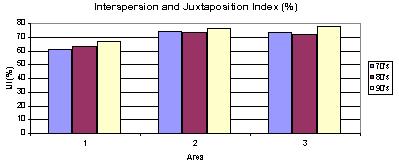
40 these LEIs also correspond to the indexes that the US Environmental Protection Agency rated 2 as "ready for field test and implementation" (EPA 1994). A large group of LEIs attempts to describe spatial characteristics of individual patches. Other indexes evaluate neighbourhood properties without explicit reference to patches, using only the grid (or pixel) representation. Patch characteristics of an entire landscape are sometimes reported as a statistical summary (e.g., mean, median, variance, and frequency distribution) for all patches of a class. When the configuration of a single patch type is of particular interest, these analyses are often conducted on binary maps (class-of-interest vs. everything else). Patch-based LEIs include size, number and density of patches (O'Neill et al., 1988). These measures can be computed for all classes together or for a particular class of interest. Useful edge information may include perimeter of individual patches, total perimeter of all patches of a particular class, the frequency of specific patch adjacencies, and various edge measures that incorporate the contrast (degree of dissimilarity) between a patch and its neighbours. Patches can take an infinite variety of shapes. Most shape indexes use a perimeter/area relationship (for which a circle, having the largest ratio, becomes the "unit object"). For example, fractal dimension describes a scale invariant power relationship between perimeter and area: P = ka D/2 Eq where P is the perimeter, A is the area of a patch, D is the fractal dimension and k is a constant of proportionality. From Eq.4.1 the fractal dimension can be determined as follows: D = 2(lnP - lnk)/lna Eq with values of D ranging between 1 for simple shapes and 2 for complex shapes (O'Neill et al. 1988, Frohn, 1997). A widely used index related to both patch-size and shape is core area (interior). Core area is the portion of a patch that is further than some prespecified distance from an edge and presumably not influenced by edge effects. It can be used as a measure of spatial heterogeneity and can function equally well as a landscape-level or patch-level index. The interspersion and juxtaposition index (McGarigal-Marks, 1995) measures the extent to which patch types (patches of different classes) are interspersed. It is conceptually similar to the pixel-based contagion index (see below), but rather than evaluating the "clumpiness" of the landscape, it measures the frequencies of patch adjacencies. 2 The other two rankings were "requiring further testing for sensitivity" and "requiring further conceptual development". Landcover Analysis of the Moose River Basin 4-4

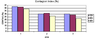
41 The most commonly used pixel-based neighbourhood index is contagion (O'Neill et al., 1988) designed to quantify both composition and configuration (Li-Reynolds, 1993): CONT = C C 2 ln(c ) + (( n ij )ln( n ij )) i =1 j=1 N N 2ln(C ) Eq where C is the number of classes, n ij is the number of shared pixel edges between classes i and j and N is twice the number of total pixel edges due to "double counting" (i.e., every edge is counted twice as AB and BA, for example). Lower values of contagion indicate many small patches, and thus the proportion of pixels being adjacent to a given landcover type are nearly equal. As there are larger contiguous patches on the landscape, contagion approximates 1. There are also class-specific contagion measures (Gardner-O'Neill, 1991) and variable size moving windows have also been introduced (Baker-Cai, 1992). An additional attractive feature of contagion and related indexes is their close relationship to classical spatial statistical measures such as the join-count statistics (Cliff-Ord, 1981, Cressie, 1990, Csillag-Fortin, 2000) Moose River Basin landcover and change analysis All nine landcover datasets were analyzed using FRAGSTATS (McGarigal-Marks, 1995). Based on the assessment of the landcover maps (Section 3.3), two series of analyses have been completed: (1) the originally produced landcover data sets were characterized by a series of LEIs, and (2) ten "no change" classes were created by merging the 25 categories (see Table 4.2) and the spatial resolution was changed to 100 m by resampling according to the "majority" rule (i.e., each 1 ha pixel inherited the most frequent category from its four "parent" pixels). The former data set will be referred to as "raw cover type" level (RCT), the latter will be referred to as "generalized cover type" level (GCT). Table 4.2. Definition of the 10 Generalized Cover Types (GCT) from the 25 Raw Cover Types (RCT) Generalized Cover Type Merged Raw Cover Types Class 2 Deciduous = 2 Class 3 Mixed deciduous = Class 4 Mixed conifer = Class 5 Conifer = 5+15 Class 6 Wetland = Class 7 Cuts = Class 8 Burns = 11 Class 9 Agriculture = 9 Class 10 Barren = 10 Class 11 Urban = 12 Landcover Analysis of the Moose River Basin 4-5

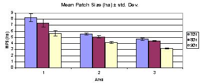
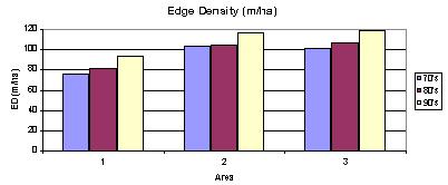
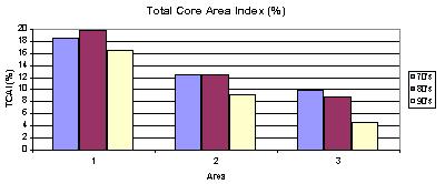
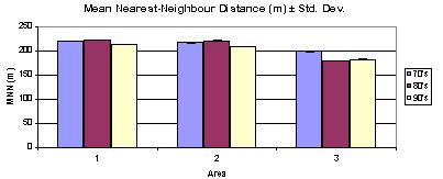
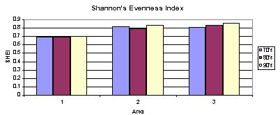
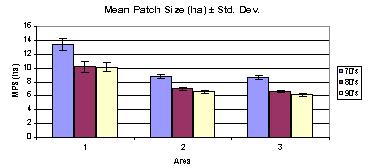
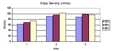
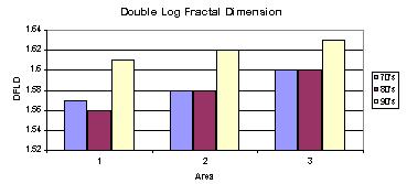
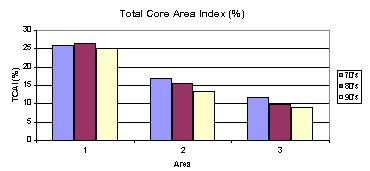
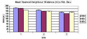
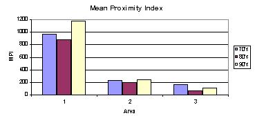
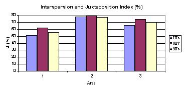
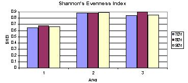
42 Landscape pattern analysis of raw cover types The landcover categories mapped according to Section 3.3. exhibited unexpectedly high variations over time. Forest covers at the RCT-level did not change in a consistent manner; in Area-1 (northern) wetlands, in Area-2 (middle) agriculture, in Area-3 (southern) cuts increased most markedly. The changes appear to be more pronounced in the second decade (1980's to 1990's), but the interpretation of the change categories is too vague without strong ground data support. Table 4.3. Landscape ecological indexes (LEIs) at the RCT-level for the MRB (3 areas by 3 dates) Area 1 Area 2 Area 3 Indices 70's 80's 90's 70's 80's 90's 70's 80's 90's Patch Density Mean Patch Size Edge Density Double Log Fractal Dim Total Core Area Index Mean Nearest-Neighbour D Mean Proximity Index Patch Richness Shannon's Evenness Index Interspersion & Juxtaposition Contagion Index Patch Size Std. Dev Nearest-Neighbour Std.Dev The instability of the RCT-level classification can be illustrated by one of the forest cover types. Coniferous forest (class 5) in Area-1 was 81,888 ha. Two state-changes appear to be possible: to mixed conifer (class 14), or to cuts (class 21), or it would remain in the same class. Following this logic, the 20,612 ha increase in the first decade, and the 6465 increase in the second decade is unexplainable. Although the pixel-by-pixel identification of landcover at the RCTlevel does not support an easy interpretation of landscape dynamics, the overall pattern of the landscape can still be analyzed by the LEIs described in Section 4.2. All analyses (summarized in Table 4.3. and Figure 4.1) were completed at landscape-level (i.e., summarizing all categories) and at cover-type level (i.e., each category is analyzed separately), but detailed interpretation could be completed only at the landscape-level Overall spatial heterogeneity of the landscape was assessed by LEIs of patchiness and isolation. Patchiness was estimated by patch density, mean patch size, edge density, total core area index, and contagion. Increases in patch density and edge density indicate a trend of the Landcover Analysis of the Moose River Basin 4-6

43 landscape becoming progressively "patchy", i.e., the likelihood of finding edges in any neighbourhood increased on average. Similar conclusion can be confirmed by the decreases in total core area index, mean patch size and contagion. Isolation was estimated by mean nearest neighnourhood distance and mean proximity index. Unlike the LEIs characterizing patchiness, these indexes have not changed markedly over the two decades. Contagion also exhibits an apparently insignificant trend. The geometrical complexity of the areas, characterized by the fractal dimension, have increased in the second decade (1980's to 1990's) in all three areas. However, spatial interspersion and cover type dominance (c.f. evennes index) apparently have not changed. Diversity in the areas have not changed except in Area-3 during the second decade (1980's to 1990's). At the cover-type level the analyses were focussed on the forest categories. Mean patch size of both dense coniferous forest and dense deciduous forest has increased. Mean patch size of cuts has also increased in the second decade (1980's to 1990's) in the two areas where they were present. All other cover-type level analyses leads to inconclusive results Landscape pattern analysis of generalized cover types The generalized cover types provide a more robust temporal profile for the changes in LEIs than the raw cover types, because they are less sensitive to local bias (i.e., inconsistencies cancel out). Although the forest cover types show extreme and some unexplainable fluctutations, the general trends in composition and pattern can be summarized as follows (Table 4.2, Table 4.3 and Figure 5.2). There is clear indication that the most extreme changes occurred in Area-2. Although the compositional changes can not be fully attributed even according to the generalized cover types, the second decade (1980's to 1990's) shows for Area-1 a decrease in mixed deciduous forest and an increase in wetlands, for Area-2 a shift from mixed forests toward deciduous and coniferous forests accompanied by a slight increase in cuts, for Area-3 a significant increase in cuts paralleled by a decrease in water surfaces and a decrease in forest cover. Landcover Analysis of the Moose River Basin 4-7

44 Figure 4.1. Landscape ecological indexes at the RCT-level for the MRB (3 areas by 3 dates). Landcover Analysis of the Moose River Basin 4-8

45 Table 4.2. Distribution of GCTs by area, by date, and by time-step Class 70's 80's 90's 70's to 80's 80's to 90's 70's to 90's AREA Class 70's 80's 90's 70's to 80's 80's to 90's 70's to 90's AREA Class 70's 80's 90's 70's to 80's 80's to 90's 70's to 90's AREA Generalized Classes: 1 - Water 7 - Cuts 2 - Deciduous Forest 8 - Burns 3 - Mixed Forest Deciduous 9 - Agriculture 4 - Mixed Forest Conifers 10 - Barren 5 - Conifer Forest 11 - Urban 6 - Wetland no data Landcover Analysis of the Moose River Basin 4-9

46 Table 4.3. Landscape ecological indexes for generalized cover types Area 1 Area 2 Area 3 Indices 70's 80's 90's 70's 80's 90's 70's 80's 90's Patch Density Mean Patch Size Edge Density Double Log Fractal Dimension Total Core Area Index Mean Nearest-Neighbour Distance Mean Proximity Index Patch Richness Shannon's Evenness Index Interspersion and Juxtaposition Contagion Index Patch Size Std. Dev Nearest-Neighbour Std. Dev Findings about landscape-scale patterns are similar in tendency to the RCT-level analysis. The apparently consistent increase in patch density and edge density with simultaneous decrease in mean patch size and total core area index is characteristic for all three areas and strongly indicate the process of increasing spatial heterogeneity. There is also a north-south trend: northern landscapes have larger patches, less edge, less complexity, less isolation, less interspersion and more contiguity. Although, due to the unknown amount of uncertainty in the cover type identification, it is impossible to confirm the role of management in the interpretation of these findings, they seem to parallel reports about harvesting practices altering landscape patterns (Franklin-Forman, 1987), regional hydrology (Jones- Grant, 1996), biological diversity (Rosenberg-Raphael, 1986) and the carbon cycle (Cohen et al., 1996). Cover-type scale analysis suggests that the mean patch size of cuts increased particularly in the second decade (1980's to 1990's). The total core area index for cuts also increased, but did not show a consistent pattern for other generalized cover types. Landcover Analysis of the Moose River Basin 4-10

47 Figure 4.2 Landscape ecological indexes at the GCT-level for the MRB (3 areas by 3 dates). Landcover Analysis of the Moose River Basin 4-11

48 5. CONCLUSIONS AND RECOMMENDATIONS 5.1. Overview The "Moose River Landcover Analysis" project has attempted to develop, implement and demonstrate an integrated quantitative approach to operationally linking pattern and process at the landscape level. This study required us to harmonize current scientific understanding of landscape-level processes and the available modern data collection (remote sensing) and information management (GIS) technology. The most significant result of this project is a reproducible approach toward the landcover classification of Landsat imagery that can be directly input to software to produce landscape ecological indexes. As usual, there are two types of constraints on the quality of the results: one of them is the accuracy of the models and methods, the other one is the quality of the data. The more one knows (e.g., about the causes and types of landscape heterogeneity), the further one can get in building a diagnostic model and/or verifying a predictive one. There is inherent uncertainty related to spatial, temporal and thematic resolution of the data (Quattrochi- Goodchild, 1997); this particular study faced the problems related to finding a suitable thematic level of detail for coarse temporal and fine spatial resolution data Advantages and disadvantages of the MRB landcover database Sustainable forest management goals require the long-term monitoring and modeling of extensive landscapes at fine spatial and temporal resolution. Natural (climate change, fire) and anthropogenic disturbances cause changes in landscape-level heterogeneity. Landscape ecological indexes have been proven to quantitatively measure such characteristics based on categorical maps of landuse/landcover (EPA 1994, Sachs et al., 1998, O'Neill et al., 1999). This project has resulted in a georeferenced database for three test-areas in the MRB) at consistent thematic and spatial resolution to map and model decadal changes in landscape pattern. We have developed consistent methodology for multitemporal classification (including natural and anthropogenic disturbances). The output of these landcover classifications were directly input into software for the computation of landscape ecological indexes that describe landscape patterns. These indexes of landscape pattern can then be interpreted over time and across regions. Landcover Analysis of the Moose River Basin 5-1

49 80 70 reflectance TM1 TM2 TM3 TM A A A A3 Figure 5.1. Recognition likelihoods (white=1, black=0) of the "coniferous forest" type across dates and test-areas. The top two images represent Area-1 ( and ), the bottom left image represents Area-2 (850529) and the bottom right image represents Area-3 (940911). The bottom panel summarizes the class training statistics for TM1-TM4. Landcover Analysis of the Moose River Basin 5-2