Tutorial 10 - PMP Estimation

Transcription

1 Tutorial 10 - PMP Estimation In Australia, the Probable Maximum Precipitation (PMP) storms are estimated using three generalised methods: Generalised Short Duration Method (GSDM) for short durations. Generalised Southeast Australia Method (GSAM) for longer durations used in southeast Australia. Generalized Tropical Storm Method (GTSMR) for longer durations used in parts of Australia affected by tropical storms. PMP is defined by the Manual for Estimation of Probable Maximum Precipitation (WMO, 1986) as "The greatest depth of precipitation for a given duration meteorologically possible for a given size storm area at a particular location at a particular time of the year, with no allowance made for long-term climatic trends." Generalised Methods of estimating PMP use data from all available storms over a large region and include adjustments for moisture availability and differing topographic effects on rainfall depth. The adjusted storm data are enveloped by smoothing over a range of areas and durations. Generalised methods also provide design spatial and temporal patterns of PMP for the catchment. More detailed information can be found in the following website. The storms with return periods within 100 years and PMP are estimated using the method provided in ARR 1997 (Estimation of Large to Extreme Floods Book Six, ARR 1997). While xprafts can estimate the PMP values automatically, you need to specify the return period and duration. Back to: Getting Started with xprafts Section Pages Tutorial 1 - An Overview of xprafts Tutorial 2 - Basics of xprafts Tutorial 3 - Input Variables Tutorial 4 - Creating a Simple Network Tutorial 5 - Linking to External Databases Tutorial 6 - Subdivision - Pre Development Tutorial 7 - Subdivision - Post Development Tutorial 8 - River Example Tutorial 9 - Detention Basin Versus On Site Detention Tutorial 10 - PMP Estimation This tutorial details the step by step procedure of estimating PMP using xprafts for the GSAM Sample B catchment (refer to Guidebook to the estimation of PMP GSAM, Bureau of Meteorology, 1997). The catchment is located in Northeast Victoria with a total area of 436 km 2. The catchment lies in the GSAM inland application zone, and GSDM needs to be calculated since the area of the catchment is less than 1000 km² (refer to the following images from the Guidebook to the estimation of PMP GSAM, Bureau of Meteorology). The Latitude and Longitude of the centroid of the catchment are: 36deg19 S and 146deg36 E, respectively and it falls under Zone 2 for Australian Rainfall Temporal Pattern. In this tutorial, you will learn to: Create a file from Template Load Background Image and Catchment Extent Create Subcatchments Create Catchment Collection Points Set up Spatial Distribution for Short Duration PMP Use the Automated Storm Generator Set up GSDM Data for Shorter Duration Storms Set up GSAM Data for Longer Duration PMP Set up GTSMR Data for Longer Duration PMP Analyse the Results In this tutorial, you will simulate the design rainfall events for 5, 20, and 100 years return period and PMP. The durations of the design storms are 15 min, 1 hr, 2 hr, and 1 day. It means that 4 events x 4 durations = 16 design storms will be simulated.

2 Generalised Method Zones for GSAM and GTSMR, (Source: The Estimation of Probable Maximum Precipitation in Australia: Generalised Southeast Australia Method Bureau of Meteorology) GSDM (Source: Guidebook to the Estimation of Probable Maximum Precipitation: Generalised Southeast Australia Method Bureau of Meteorology) Location of the catchment (Source: Google Earth)

3 The data/files supplied to complete this tutorial are: File Name Type Description Aerial_Image.jpg Image file Aerial image of the project area Aerial_Image.jpw World coordinate file File associated with the image file PMP.xpt XP Template file Contains temporal pattern for PMP, default job control settings, global databases, etc Catchment_B_Extent.xpx XPX file Contains the extent of the catchment B You can use *.shp, *.dwg, *.dxf, or image files to digitize the catchments. Creating the File from Template First, you need to create the file using the PMP.xpt template. 1. Open xprafts. Go to File > New > Create from Template. Name the model PMP.xp and S ave in your desired location. 2. Now xprafts asks you to select the template in the Template folder in the installed directory by default. Choose the template named PMP.xpt and then click Open. The PMP.xpt file contains the GSDM, GSAM, and GTSMR temporal patterns and the IFD data for the study area. Loading Background Image and Catchment Extent Add a new background image Aerial_Image.jpg (follow procedure described in section Add ing a Background Image and the Zoom Tool in Tutorial 6). Load the catchment extent called Catchment_B_Extent.xpx. Go to File > Import Data, bro wse for the file and then click Open. In this example, the catchment has been made available for training purposes.

4 2. 3. You need to create the catchment if it is not available by using the Create Subcatchment tool. Alternatively, you can go to PMP in the main menu, select Catchment Extent > Create, and then digitize the catchment. You need define the whole catchment, as well as sub-catchments as represented in the next section. Creating Subcatchments Digitize three sub-catchments, as shown in the following figure, using the Create Subcatchment to ol. Alternatively, you can add *.shp, *.mif, *.dwg files as catchment background images and digitize the catchments using the Create Subcatchment tool.

5 Creating Catchment Collection Points 1. Add nodes in the catchments outlet points using the Node tool, then connect these nodes (from Node 1 to Node 3) using the Link tool. 2. Now, you need to connect the catchments to the outlet nodes. Make sure that the Catchments tool Lock is switched-off when connecting the catchments to the collection points. Select the Point er tool and click the catchment. The cursor changes as shown in the image below. Keep the left button pressed and release it when the cursor reaches the outlet node. Select the Drain Catchment As > Subcatchment1.

6 Repeat this step for all the other catchments. 3. Select all the nodes by clicking the Select all nodes tool. Go to Tools menu, select Calculate Node and then click Catchment Area. The catchment areas are then calculated and assigned as FIRST Subcatchment to the nodes.

7 4. 5. Click OK and return to the main network window. Double-click any node to open the Node Control Data dialog and select Subcatchment Data. Click the FIRST Subcatchment button. You can see that the calculated area is assigned in Total Area to the node.

8 6. Double-click link 1 to open the Link Lagging dialog and enter LAG as 200 min. Similarly, enter the LAG for link 2 as 350 min. Click OK after you have finished Now, add a loss model to the subcatchments. Go to Configuration > Global Data and highlight Init./Cont. Losses. Click New and enter the name as NoInfil.

9 9. Click Edit and enter the values of 0 for both Initial Loss and Continuing Loss of Absolute. 10. Click OK to return to the main network window. Setting up Spatial Distribution for Short Duration PMP GSDM Ellipses are used to establish the spatial distribution of PMPs for shorter durations.

10 1. Go to PMP in the menu bar, select GSDM Ellipses > Show Ellipses. 2. You can see the 10 ellipses on the screen now (A J) and the center point of the ellipses as a small circle. The next step is to overlay the ellipses with the catchment outline by moving and rotating to obtain the best fit by the smallest possible ellipse. To do this, click the Center Circle of the ellipses and hold left mouse. Now, you are able to move the ellipses. To rotate the ellipses, press Shift on the key board While moving and rotating the ellipses, you are able to see the PMP Monitor dialog which shows the GSDM spatial distribution calculations. To see this monitor, click PMP in the menu bar, select GSDM Ellipses > Show PMP Calculations. Go to PMP > GSDM Ellipses and then select Lock Ellipses. You can see that the ellipses are locked and cannot be moved. You can lock the nodes and catchments as well using the Lock Node Positions and Lock Catchment tools respectively. Using the Automated Storm Generator

11 Automatic Storm Generator is used for generating storms with any storm durations and any return periods. Storms up to 100 years return period is estimated using the IFD coefficients, rainfall duration, and temporal pattern depending upon the zone (AR&R, 1987). 1. To activate the Automatic Storm Generator, go to Configuration > Job Control. Alternatively, click the Job Control icon 2. and select Job Definition. Click the Automatic Storm Generator radio button. 3. Now you can see the Global Storm Generator dialog. Click the Global Storms tab.

12 4. Click IFD and select the global database for IFD coefficients called Albury. The Albury data is included in the template file PMP.xpt and represents the IFD coefficients for the region. 5. Click Edit and you can see the IFD coefficients for the project area. You can get the IFD coefficients from the ARR 1987, Volume 2. Design rainfall isopleths maps are available for 2 and 50 years for 1, 12, and 72 hours

13 durations. Location skewness and geographical factors are also available in the ARR volume. Otherwise, you can get these coefficients from the Australian Bureau of Meteorology website. 6. Click OK. Select Albury and click Select in the dialog box. 7. In the Global Storm Generator dialog, enter the Zone as 2, as the study area is under zone 2 of the Australian rainfall temporal pattern. Refer to the following figure given by ARR 1987: Design Rainfall Temporal Pattern Zones for Australia (Source: ARR 1987, BOM) Under Storm Duration select 15, 60, 120, and 1440 min. 10. In the Global Storm Generator dialog, under Time Control, enter Routing Increment as 1 min. Under Simulation Time enter Simulation Time = Storm Duration x 1. Under Return Period select 5, 20, 100, and PMP and then click OK. When you select PMP as return period, 10, 20, 25 min Storm Durations will be greyed out automatically as PMPs will not be calculated for these durations. Now xprafts calculates 4 events x 4 durations = 16 design storms chosen for the catchment. The temporal patterns up to 100 year return period are stored in the program. The engine picks up the corresponding temporal pattern for a storm depending upon the zone, return period, and duration. However, you should specify the temporal patterns for the PMP. For GSDM, there is a single temporal pattern (up to 3 or 6 hours).

14 Temporal Pattern for PMP for short durations (Source: the Estimation of Probable Maximum Precipitation in Australia: Generalised Short-Duration Method, BOM, 2003) There are different temporal patterns for GSAM and GTSMR depending on the catchment area and storm duration. The temporal pattern for GSAM and GTSMR starts at 24 hours. You should estimate the in-between values (3-24 hours) as described in the GSAM and GSTMR Guidebooks from Bureau of Meteorology. Setting up GSDM Data for Shorter Duration Storms Go to Configuration in the main menu and open Job Control. Click Automatic Storm Generator and then select the PMP tab. You can see that the Total Area of the catchment is automatically calculated. Now enter L atitude of and Longitude of for the catchment centroid. These values will be used in calculation of adjustment factors for GSAM and/or GTSMR. Enter PMP Return Period of years. The data will be used to interpolate values between 100 years and PMP (for example, 150 or 200 year return period) Under GSDM - Generalized Short Duration Method, select Duration Limit as < 3 hr fro m the drop down list. Click Temporal Pattern and select GSDM from the global database imported from the PM P.xpt file, and then click Select. There is only one temporal pattern for the short duration PMP estimation that is

15 GSDM. 6. Click GSDM Worksheet to open Global Storms Summary for GSDM and enter the following values: Smooth (S) (smooth fraction of terrain) as 0 EAF as 1 MAF as 0.60 Refer to the Estimation of Probable Maximum Precipitation in Australia: Generalised Short-Duration Method (BOM, 2003) for more details about terrain types and adjustment factors. The paragraph below is cited in the guidebook: Rainfall from single, short duration thunderstorm events is not significantly affected by the terrain. Therefore, it is not necessary to classify the terrain of the catchment for durations of an hour or less. If durations longer than one hour are required, the next step is to establish the terrain category of the catchment and to calculate the percentages of the catchment that are rough and smooth. Rough terrain is classified as that in which elevation changes of 50 m or more within horizontal distances of 400 m are common. Rough terrain induces areas of low level convergence which can contribute to the development and redevelopment of storms, thereby increasing rainfall in the area over longer durations. Terrain that is within 20 km of generally rough terrain should also be classified as rough. If there is smooth terrain within the catchment that is further than 20 km from generally rough terrain, an areally weighted factor of rough (R) and smooth (S) terrain should be calculated such that R plus S equals one. If a catchment proves difficult to classify under these guidelines then the whole catchment should be classified as rough. The mean elevation of the catchment should be estimated from a topographic map. If this value is less than or equal to 1500 m the EAF is equal to one. For elevations exceeding 1500 m the EAF should be reduced by 0.05 for every 300 m by which the mean catchment elevation exceeds 1500 m. For most catchments in Australia the EAF will be equal to one.

16 Moisture Adjustment Factor (Source: GSDM Guidebook, BOM) 7. Click Update under the GSDM tab in the Global Storms Summary dialog. You see that the GSDM PMP depths are estimated from Equation (in the PMP Values (mm) table) up to 3 hours as you specify the duration limit to < 3 hrs. The Initial Depth Smooth (Ds) in the PMP Values (mm) table for the Smooth Terrain calculated are 0.

17 8. 9. Click OK in the Global Storms Summary dialog. Go to Apply Spatial Factors in the Global Storm Generator dialog. Select Compute for All Durations and click OK. This is now applying spatial variation to sub-catchments based on their coverage of the GSDM ellipses.

18 Setting up GSAM Data for Longer Duration PMP Go to Configuration in the main menu and open Job Control. Click Automatic Storm Generator and then select the PMP tab. Under Long Duration PMP Method, select GSAM. In GSAM Zone, select Inland from the drop down list. 5. Now, you need to specify the Temporal Pattern for the 24 hours GSAM PMP Storm. Sele

19 ct GSAM_I500_24 as the temporal pattern (that is, GSAM, Inland, 500 km2, 24h hours). Click Select. You do not need to specify the temporal pattern for 15, 60, and 120 min PMP storms as they fall under short durations, hence the GSDM temporal pattern will be applied. 6. Click Global Storms Summary and select the GSAM tab.

20 7. Under CATCHMENT FACTORS, click Compute under Topographic Adjustment Factor (TAF) and TAF will be calculated based on the entered latitude and longitude. 8. Similarly, click Compute under EPW Seasonal catchment average to calculate for Sum mer and Autumn. Alternatively, you can directly enter the values of TAF and EPW. xprafts calculates the TAF and EPWs values based on the latitude and longitude of the catchment centroid. It will be more accurate if the average value for the catchment is calculated by overlaying the catchment outline on the TAF and EPWs grids as described in the GSAM Guidebook.

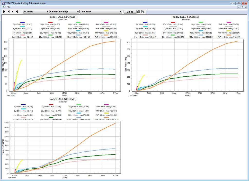
21 9. Click Update in the Global Storms dialog and you can now see that FINAL GSAM PMP ESTIMATES are calculated. Setting up the GTSMR Data for Longer Duration PMP For Catchment B, the GTSMR estimation is not required. However, for some other catchments GTSMR estimation will be required based on the location. You can follow the same procedure that is provided for the GSAM. For some catchments, both GSAM and GTSMR will be applicable, for example, GSAM-GTSMR Coastal Transition Zone. In this case, the PMP depths should be estimated by both methods and the maximum value is selected. Analysing the Results Click Solve to simulate the model. To review results, select the nodes that you wish to see the results and click Review Results.

22