UKnowledge. University of Kentucky. Jann E. Fry University of Kentucky, Recommended Citation

Transcription

1 University of Kentucky UKnowledge Theses and Dissertations--Biology Biology 2014 A PLANT TRAIT-BASED APPROACH TO EVALUATE THE ABILITY OF NATIVE C 3 AND C 4 GRASSES TO RESTORE FUNCTIONALITY TO A REMNANT BLUEGRASS SAVANNA-WOODLAND IN KENTUCKY, USA. Jann E. Fry University of Kentucky, jann.fry@gmail.com Click here to let us know how access to this document benefits you. Recommended Citation Fry, Jann E., "A PLANT TRAIT-BASED APPROACH TO EVALUATE THE ABILITY OF NATIVE C 3 AND C 4 GRASSES TO RESTORE FUNCTIONALITY TO A REMNANT BLUEGRASS SAVANNA-WOODLAND IN KENTUCKY, USA." (2014). Theses and Dissertations--Biology This Doctoral Dissertation is brought to you for free and open access by the Biology at UKnowledge. It has been accepted for inclusion in Theses and Dissertations--Biology by an authorized administrator of UKnowledge. For more information, please contact UKnowledge@lsv.uky.edu.

2 STUDENT AGREEMENT: I represent that my thesis or dissertation and abstract are my original work. Proper attribution has been given to all outside sources. I understand that I am solely responsible for obtaining any needed copyright permissions. I have obtained needed written permission statement(s) from the owner(s) of each thirdparty copyrighted matter to be included in my work, allowing electronic distribution (if such use is not permitted by the fair use doctrine) which will be submitted to UKnowledge as Additional File. I hereby grant to The University of Kentucky and its agents the irrevocable, non-exclusive, and royaltyfree license to archive and make accessible my work in whole or in part in all forms of media, now or hereafter known. I agree that the document mentioned above may be made available immediately for worldwide access unless an embargo applies. I retain all other ownership rights to the copyright of my work. I also retain the right to use in future works (such as articles or books) all or part of my work. I understand that I am free to register the copyright to my work. REVIEW, APPROVAL AND ACCEPTANCE The document mentioned above has been reviewed and accepted by the student s advisor, on behalf of the advisory committee, and by the Director of Graduate Studies (DGS), on behalf of the program; we verify that this is the final, approved version of the student s thesis including all changes required by the advisory committee. The undersigned agree to abide by the statements above. Jann E. Fry, Student Dr. Scott K. Gleeson, Major Professor Dr. David Westneat, Director of Graduate Studies

3 A PLANT TRAIT-BASED APPROACH TO EVALUATE THE ABILITY OF NATIVE C3 AND C4 GRASSES TO RESTORE FUNCTIONALITY TO A REMNANT BLUEGRASS SAVANNA-WOODLAND IN KENTUCKY, USA. DISSERTATION A dissertation submitted in partial fulfillment of the requirements for the degree of Doctor of Philosophy in the College of Arts and Sciences at the University of Kentucky By Jann E. Fry Director: Dr. David Westneat, Professor of Biology Lexington, Kentucky Copyright Jann Elise Fry 2014

4 ABSTRACT OF THESIS A PLANT TRAIT-BASED APPROACH TO EVALUATE THE ABILITY OF NATIVE C3 AND C4 GRASSES TO RESTORE FUNCTIONALITY TO A REMNANT BLUEGRASS SAVANNA-WOODLAND IN KENTUCKY, USA. Temperate Midwestern oak savannas are considered imperiled ecosystems with < 1 % remaining since European settlement and are identified as critical areas for preservation. Restoration of Midwestern oak savannas is challenging due to several factors including lack of accurate historical data, few intact remnants remaining to study, and lack of restoration ecology studies. A plant trait-based approach was used to evaluate the ability of six C 3 and three C 4 native bunchgrasses to restore functionality to a remnant savanna woodland of the Bluegrass Region of Kentucky. The response and effect framework was used to assess the response of the nine native grasses according to the habitat filters of interannual precipitation, inter- vs. intra-specific competition, and simulated grazing. The effect traits associated with plant-soil nitrogen and carbon cycling were also assessed. The response traits of interannual competition and inter- vs. intra-specific competition along with the effect traits plant-soil nitrogen and carbon cycling were measured in a monoculture experiment conducted at Griffith Woods WMA. The simulated grazing or clipping experiment was conducted over three months in a heated greenhouse experiment. Four of the C 3 species were of the genus Elymus which had significant differences in life history traits compared to the other species made them particularly well adapted to the Bluegrass Savanna- Woodland. The Elymus species were not well adapted to the most intense clipping treatment (clip to 7 cm). For the other two C 3 species, C. latifolium would be a better competitor than D. clandestinum under normal conditions. D. clandestinum had the most number of plastic traits and was the only species to exhibit all three grazing strategies. Comparing the C 4 species, T. flavus and P. anceps grew well in the monoculture but A. virginicus did not. The life history traits of A. virginicus does not make this species a good candidate for restoration at this site. The three C 4 species were well adapted to clipping. The results of this study suggest that the C 3 species, particularly the Elymus, are well adapted to the eutrophic mesic conditions of the Bluegrass Savanna-Woodland, and that the C 4 species are better adapted to disturbance. KEYWORDS: savanna, restoration ecology, C 3 and C 4 grasses, response traits, effect traits.

5 A PLANT TRAIT-BASED APPROACH TO EVALUATE THE ABILITY OF NATIVE C 3 AND C 4 GRASSES TO RESTORE FUNCTIONALITY TO A REMNANT BLUEGRASS SAVANNA-WOODLAND IN KENTUCKY, USA. By Jann Elise Fry Dr. Scott K. Gleeson n Director of Dissertation Dr. David Westnest t Director of Graduate Studies May 1, 2014

6 ACKNOWLEDGMENTS This project has benefited from the help of many people. I would like to thank my committee for guiding me through this process. Dr. Scott Gleeson for believing that I was capable of getting my Ph.D. Dr. Tim Phillips advised me on how to get these grasses to grow and when and how to plant them. He had a major input on the design of the clipping experiment. Dr. Rebecca McCulley also helped in the design of the experiments especially the plant-soil N and C cycling experiment. I also got valuable feedback from the Dr. Rebecca McCulley s and Dr. Mary Arthur s regular lab group meetings. Dr. Carol Baskin gave me good advice and edited my entire manuscript. The help of Jyotirekha Chakravarty for two years had a big impact on my research. She was instrumental in setting up and collecting data for the clipping experiment, the monoculture experiment, and the light gradient experiment. Dr. Julian Campbell helped me choose the species to use in my experiments, helped me collect seed, and watered my plants in the field when needed. His insights were very helpful. Jim Nelson was instrumental in helping me run samples for the palatability study, ash free weights. He also gave me statistical help and advice. Last but not least, I would like to thank my family which has supported me through this process. My husband, John, was indispensable as he mowed the fields, built my shade structures, helped me print many labels, scanned leaves, encouraged me to graduate, among many other things too numerous to name. I hope my children benefit from watching me go through this process. I am the first person in my extended family to earn a Ph.D. iii

7 Table of Contents ACKNOWLEDGMENTS... iii Chapter 1: Introduction... 1 Tables... 7 Figures... 7 Literature Cited... 8 Chapter 2: Do C 3 and C 4 bunchgrasses differ in phenotypic plasticity and stress tolerance in response to drought and competition? Abstract Introduction Materials and Methods Study Site Species Experimental procedures Results Species performance Drought effects Competition x drought Discussion Literature Cited Tables Figures Chapter 3: Differences in ecosystem properties between C 3 and C 4 grasses native to a historic North American Oak Savanna Abstract Introduction Materials and Methods Study Site Species Experimental procedures Results Species characteristics Litter Decomposition Nitrate and ammonium resin data iv

8 Soil data Discussion Literature Cited Tables Figures Chapter 4: Grazing strategies of C 3 and C 4 bunchgrasses native to a historic Oak Savanna-Woodland Abstract Introduction Methods Experimental Design Plant traits Statistics Results Group, Species and Treatment Effects:ANOVA Group, Species and Treatment Effects:PCA Species Differences at each Treatment Level Treatment Differences for each Species Grazing strategies Discussion Grazing strategies Conclusion Literature Cited Tables Figures Chapter 5: Conclusion Literature Cited Curriculum Vitae v

9 Chapter 1: Introduction Savannas are grassland ecosystems characterized by the trees being either small or widely spaced so that the tree canopy is not closed (McPherson 1997), and are influenced by fire, climate, topography and soil type (Nuzzo 1986). Savannas cover 20 % of the Earth s land area and can be divided into tropical and temperate groups. Tropical savannas cover 15 % of the Earth s land area, are generally better represented in the scientific literature, and are extensive in Africa, Australia, and S. America (McPherson 1997). While temperate savannas of North America were historically common at the time of European settlement, most of these landscapes have been reduced to < 1 % of their original area, are considered to be endangered (Anderson, Fralish et al. 1999), and are identified as critical areas for preservation (Klopatek et. al 1979). Furthermore, temperate savannas are not as well studied or represented in the scientific literature as tropical savannas (McPherson 1997, Anderson, Fralish et al. 1999). At the time of European settlement of Midwestern North America, oak savannas occurred in the northern half of the central United States in a region that includes Minnesota, Iowa, Missouri, Wisconsin, Illinois, Michigan, Indiana, and Ohio (Nuzzo 1986). The oak savanna was mainly a transitional community located between the western prairie and eastern deciduous forest (Nuzzo 1986, McPherson 1997). The dominant trees were primarily Quercus sp., giving rise to names for the savanna such as oak savanna and oak savanna-woodland. Bray (1960) and Nuzzo (1986) characterized open savannas as usually dominated by burr oak (Quercus macrocarpa) and primarily found on flatter more mesic areas than scrub savannas. Scrub savannas were dominated by white oak (Quercus alba) and black oak (Quercus velutina) and were generally found on dry to dry-mesic areas of steeper topography. Within 20 to 40 years, after the Midwest was settled by Europeans in the eighteenth century, oak savannas all but disappeared due to fire cessation and conversion of land to agricultural or urban development (Nuzzo 1986, Anderson, Fralish et al. 1999). The fact that only 2% of Midwestern Oak Savannas remained by 1986 (Nuzzo 1986) has caused this habitat to be listed as a globally imperiled ecosystem (Heikens and Robertson 1994). Conservation and restoration efforts of Midwestern Oak Savannas are difficult due to: 1) the limited amount of historical data, which were recorded mainly by European pioneers and land surveyors, and the unknown validity and motivation for these records (Nuzzo 1986); and 2) the lack of restoration ecology studies that could guide ecological restoration practices and management of these systems (McPherson 1997). One potential reason for the lack of research activity on restoration of Midwestern oak savannas and temperate savannas in general, is the absence of a professional discipline associated with savannas that promotes an understanding of the role and importance of savannas in temperate regions (McPherson 1

10 1997). Since Midwestern oak savannas are generally transitional zones between grasslands and oak forests (McPherson 1997), boundaries between the three vegetation types are subjective. Midwestern oak savannas can be utilized as grasslands for grazing animal production and managed accordingly or utilized as woodlands with forest management. Another potential reason for the lack of research activity for Midwestern oak savannas could be inconsistent definitions and/or interpretations of the term savanna (McPherson 1997). Midwestern oak savannas can be referred to as oak savanna, oak opening, oak barrens, scrub prairie, brush prairie, and brush savannas (Nuzzo 1986) Thus, definitions of a Midwestern oak savanna are variable and can be site specific (McPherson 1997, Anderson, Fralish et al. 1999). Bray (1960) and Nuzzo (1986) classified Midwestern oak savannas as open savanna or scrub savanna and these two savanna types can vary over time and disturbance levels. The amount of canopy cover in Midwestern oak savannas is also highly variable. According to McPherson (1997), the woody plant cover of Midwestern oak savannas can range from < 1% to about 30%, while Nuzzo (1986) reported canopy cover of Midwestern oak savannas ranging from 10% to 100%. The species composition of the understory also determines the difference between a forest, grassland, and a savanna. Nuzzo (1986) categorized the savanna understory as having less grass and more forbs and shrubs than a prairie, but more grass and fewer forbs, vines, and shrubs than oak forests. Thus, while the definition of savannas include a grassland and tree component, savannas can broadly differ in the way they look and, most likely, the way they function. The general definition of a savanna found in most textbooks also can be misleading when identifying Midwestern oak savannas. For example, while frequent low intensity fires, a distinct annual dry season, extended droughts, and grazing by large herbivores are characteristics often associated with savannas (Enger and Smith 2004), these characteristic may be more common to African Tropical Savannas than Midwestern oak savannas (McPherson 1997). The climate of most Midwestern Oak savannas does not promote frequent low intensity natural fires or extended droughts, and the dry season is generally more variable than in tropical savannas. While natural fires may not be common in Midwestern Oak savannas, fire is considered to be an important disturbance in the maintenance of these savannas, with fires started by Native Americans playing an important role historically (Mann 2011). With the lack of research conducted on Midwestern oak savannas and few intact oak savannas remnants remaining, restoration of a functional savanna community requires an alternative approach. The plant trait-based approach views a species as a set of inter-connected traits that are both the result of its evolutionary history and determine the ability of the species to respond to or affect biotic and abiotic environmental filters (Adler, Milchunas et al. 2004). The response-and-effect framework uses this plant trait-based approach that views a species as a set of interconnected traits which can both respond to 2

11 abiotic and biotic habitat filters and can affect ecosystem properties (Garnier and Navas 2012). The response-and-effect framework includes a performance trait (e.g., annual net primary production - ANPP), which is an overall indicator of plant fitness that can be explained by morphological or physiological response traits (Garnier and Navas 2012). In this study, morphological traits are referred to as macroscopic traits since they are easily observed and measured, and physiological traits are referred to as microscopic traits since they are not easily observed or measured. Macroscopic and microscopic response trait values can vary with differing abiotic and biotic habitat filters, which can then affect traits that influence ecosystem functioning (Lavorel and Garnier 2002) through the direct effects of habitat filters as well as feedback loops that affect ecosystem function (Garnier and Navas 2012). These response and effect traits can be interrelated and may or may not be correlated (Couso and Fernandez 2012). By growing prospective species in monocultures, performance, response and effect traits can be measured to determine each species characteristics and niche which then can be used to predict how they might function in a mixed species community setting. The purpose of this restoration ecology study was to study the plant traits of six C 3 and three C 4 perennial grasses to help evaluate possible components of a restored functional grassland community for the historic Oak Savanna-Woodland located in the Inner Bluegrass Region of Kentucky, USA. The Bluegrass Savanna-Woodland was considered by Braun (1943) to be anomalous or unexpected in the middle of the mixed mesophytic forest biome. Wharton and Barbour (1991) characterized this area as a savanna-woodland with an open forest whereby the trees are dominant but with a well-developed grassy undergrowth. This savanna-woodland was described at the time of European settlement in the mid to late 1700 s as having a rolling mildly karst topography, fertile, deep, and well drained silt loam soil produced over highly phosphatic Ordovician Limestone, vast cane breaks (Arundinaria gigantea), large mature trees including oak (Quercus sp.) and ash (Fraxinus sp.), and a graminoid dominated herbaceous layer (McInteer 1952, Wharton and Barbour 1991, Campbell 2004). With European settlement, native grasses were rapidly replaced by non-native C 3 forage grasses (Poa pratensis and Festuca arundinacea) so that no intact savanna grassland remains in this region today (Bryant, Wharton et al. 1980). The native C 3 grasses were thought to be dominant in both abundance and number of species in woodlands (Wharton and Barbour 1991) with mesic eutrophic soils as well as in the more open woods (Campbell 2004). The native C 4 grasses were thought to be fewer in the number of species and found in local openings on poorer soils or openings created by disturbance such as fire or bison trails (Campbell 2004). Common prairie grasses of more western prairie regions were not common in this region (Campbell 2004). 3

12 The two experiments included in this study were a field monoculture experiment and a greenhouse clipping experiment. The monoculture experiment was conducted in a relatively flat, tall fescue (Festuca arundinacea) dominated abandoned paddock located at Griffith Woods Wildlife Management Area (WMA). Griffith Woods WMA is considered to be the best Bluegrass Savanna- Woodland remnant in the Inner Bluegrass Region of Kentucky. It includes 302 hectares in southern Harrison County, Kentucky, and lies on the northern edge of the Inner Bluegrass Region of Kentucky. While the vegetation of Griffith Woods WMA is known for its remnant Blue Ash-Oak savanna-woodland with year old trees of Fraxinus quadrangulata (Blue Ash), Quercus macrocarpa (Burr Oak), Quercus muhlenbergii (Chinquapin Oak), and Quercus shumardii (Shumard Oak), the herbaceous layer is dominated by non-native C 3 forage grasses (e.g., Festuca arundinacea and Poa pratensis). In the field monoculture experiment, characteristics for each of the nine native grass species, the performance trait of annual net primary production (ANPP), macroscopic traits and microscopic traits were measured in 2010 and Since these two years had significant differences in interannual precipitation, plant traits for each species were analyzed between the relatively dry year (2010) and the wet year (2011). A species mixture treatment was added to the monoculture experiment to compare how the species performed in the monoculture (with only intra-specific competition) and the species mixture treatment (with inter-specific competition). This comparison was analyzed for both the dry year and the wet year. Chapter 1 includes how each species performed in the monoculture in general, the response trait comparisons between the dry vs. wet year (drought effects), and the response trait comparisons between inter- vs. intra-specific competition that were measured in both the dry and wet year (competition x drought effects). This information can then be used to predict how they might function in a community setting. My hypotheses included: 1) The C 3 and C 4 grasses will differ in the macroscopic and microscopic plant traits that explain the performance trait (ANPP); 2) ANPP and macroscopic and microscopic response traits will be differentially affected by the habitat filters of drought and drought x competition; 3) In response to the habitat filter of drought and competition, the C 3 species would show trait differences in the performance trait and macroscopic traits, and that the C 4 species will be more stress tolerant and show trait differences only in microscopic traits; 4) The macroscopic and microscopic traits of the four Elymus species will not be plastic in response to drought as their plant traits were measured before the summer drought of The Elymus species should have experienced the least amount of precipitation variability as both years had a wet spring. The macroscopic and microscopic traits of the other two C 3 species that were actively grow during the summer will show plasticity in traits as they did experience summer interannual precipitation variability, and the C 4 species will be stress tolerant and only 4

13 plastic in the microscopic traits; and 5.) Drought and competition will have differing effects on C 4 and C 3 species whereby C 3 species should be at a competitive advantage over the C 4 species in the wet year (2011), and the C 4 species should be at a competitive advantage over the C 3 species in the dry year (2010). Results of this experiment can be used to better understand the dynamics of this Bluegrass Savanna-Woodland and how these nine species might perform in a mixed species community. A variety of effect traits associated with plant-soil nitrogen and carbon cycling were also assessed in the monoculture experiment and are presented in Chapter 2. The goal of this study was to determine if the species were fast N cycling or slow N cycling species and how these characteristics affected N and C soil pools and soil nutrient concentrations. Chapter 2 included species characteristics, an inorganic N resin pools, litter decomposition, and soil nutrient analyses. I hypothesized that: 1) The C 3 grasses will have plant traits that promote fast N cycling, and C 4 grasses will have plant traits that promote more conservative or slow cycling N plant traits; and 2) If N is limiting at the ecosystem level, slow N cycling species should store N in more slowly cycling, recalcitrant pools more than fast N cycling species according to the resource-competition theory. The greenhouse clipping experiment is presented in Chapter 3. If grazing was an important disturbance in the Bluegrass Savanna-Woodland, these native grasses should have evolved grazing strategies to tolerate, deter, or avoid grazing. Since savannas are maintained by disturbance, the goal of this experiment was to better understand the ability of the nine grass species to respond to grazing, and to recommend effective mowing regimes that would maintain a functional grassland community within the Bluegrass Savanna-Woodland. The clipping experiment had a factorial design with two clipping heights (intensities) and two clipping frequencies designed to mimic frequent intense grazing to less intense rotational grazing, with a non-clipped control included for comparison. I hypothesized that: 1) Frequency will have a bigger impact on plant traits than intensity as predicted by Augustine and McNaughton (1998); 2) The C 4 species will be better adapted to grazing than the C 3 grasses because they generally have higher nitrogen use efficiency, a higher C:N ratio, and a higher water use efficiency that should make them less affected by biomass loss; and 3) The grasses may employ different grazing tolerance? strategies at different frequency and intensity treatment levels. Results of this experiment can be used to recommend mowing regimes for ecological restoration that will maintain these grasses in a community setting, and provide insights for future restoration efforts. Considering the response-and-effect framework, this study measured response traits across the abiotic habitat filter of drought and the biotic habitat filters of competition and grazing, and effect traits that impacted the cycling of N and C and soil nutrient concentrations. This information was used to help inform how these nine species would perform in a community and the biogeochemical effects they might 5

14 have on the plant-soil system. The nine native species used in this study were identified as potentially good candidates for the ecological restoration of the Bluegrass Savanna-Woodland (Table 1.1). The six C 3 grasses included in this study are associated with wooded habitats, and the three C 4 species are associated with more open habitats (Wharton and Barbour 1991, Campbell 2004). Of the six C 3 species, four are from the genus Elymus or wildryes which are well documented in historical records and are thought to have been abundant at the time of European settlement in the mid to late 1700 s (Wharton and Barbour 1991). The Elymus species have a different life history pattern with significant niche differentiation from the other species. They flower in the spring or early summer, set seed, and then go dormant during the hottest months of the summer. They regrow tillers in the fall which overwinter and produce flowering culms the next spring. The Elymus species flower before the other five species (Figure 1.1). Dichantheilium clandestinum and Chasmanthium latifolium were the last two C 3 species to flower (Figure 1.1). D. clandestinum may have been referred to as buffalo grass in historical records where it is frequent in open woods, thickets, and fencerows, especially on low ground (Wharton and Barbour 1991). D. clandestinum also has life history traits that differ from the other species in this study. D. clandestinum first produces cleistogamous flowering culms, and then later in the season they produce self-fertilizing chasmogamous flowers on small inflorescences that are usually hidden within the sheathes. Both types of flowers produce viable seeds. While this species does not produce a lot of tillers, it had the greatest ability for tiller branching, so one tiller could be quite large and heavy. C. latifolium is frequent on wooded stream banks, on floodplains, and in other moist habitats (Wharton and Barbour 1991). C. latifolium is also used in horticultural plantings and can be quite invasive. The three C 4 species are generally found in more open sites and flowered after the C 3 species (Figure 1.1). P. anceps is found less commonly and on moist ground, and T. flavus is common in old fields, woodland borders, open woods, pastures, and roadsides (Wharton and Barbour 1991). Andropogon virginicus is common in old fields and overgrazed pastures and is the last of the C 4 species to bolt and produce flowering culms (Wharton and Barbour 1991). Thus, the plant trait method was used evaluate the ability of native grasses to restore functionality of the grassland component of the oak savanna-woodland in central KY. Specific hypothesis were tested in a greenhouse and field experiment, and the results provide us with new insights into how to select native grasses for use in restoration projects. 6

15 Tables Scientific Name Common Name Photosynthetic Pathway 1. Elymus macgregorii R. Brooks & J.J.N. Campb. Early wildrye 2. Elymus villosus Muhl. ex Willd. Nodding wildrye 3. Elymus virginicus L. Virginia wildrye 4. Elymus hystrix L. Bottlebrush C3 5. Dichanthelium clandestinum (L.) Gould Deer tongue 6. Chasmanthium latifolium (Michx.) Yates River Oats 7. Panicum anceps Michx. Beaked panicgrass 8. Tridens flavus (L.) Hitchc. Purple top/grease grass C4 9. Andropogon virginicus L, Broomsedge Table 1.1: The nine native perennial bunchgrass species used in this experiment listed in order of flowering time. Figures 9-Oct 19-Sep 30-Aug 10-Aug 21-Jul 1-Jul 11-Jun 22-May 2-May 12-Apr 23-Mar Peak biomass collection dates Figure 1.1: The dates of data collection according to each species time of flowering or peak biomass. 7

16 E. macgregorii E. villosus E. virginicus E. hystrix D. clandestinum C. latifolium P. anceps T. flavus A. virginicus Present absent/not reported Figure 1.2: Distribution maps for the nine species taken from the NRCS plants database. Literature Cited Adler, P. B., D. G. Milchunas, W. K. Lauenroth, O. E. Sala and I. C. Burke (2004). "Functional traits of graminoids in semi-arid steppes: a test of grazing histories." Journal of Applied Ecology 41(4): Anderson, R. C., J. S. Fralish and J. M. Baskin, Eds. (1999). Savannas, Barrens, and Rock Outcrop Plant Communities of North America. Cambridge, UK, Cambridge University Press. Augustine, D. J. and S. J. McNaughton (1998). "Ungulate effects on the functional species composition of plant communities: Herbivore selectivity and plant tolerance." Journal of Wildlife Management 62(4):

17 Bray, J. R. (1960). "THE COMPOSITION OF SAVANNA VEGETATION IN WISCONSIN." Ecology 41(4): Bryant, W. S., M. E. Wharton, W. H. Martin and J. B. Varner (1980). "The Blue Ash-Oak Savanna- Woodland, a Remnant of Presettlement Vegetation in the Inner Bluegrass of Kentucky." Castanea 45(3): Campbell, J. (2004). Comparitive Ecology of Warm-Season (C4) versus Cool-Season Grass (C3) Species in Kentucky, with Reference to Bluegrass Woodlands. 4th Eastern Native Grass Symposium University of Kentucky. Couso, L. L. and R. J. Fernandez (2012). "Phenotypic plasticity as an index of drought tolerance in three Patagonian steppe grasses." Annals of Botany 110(4): Enger, E. D. and B. F. Smith (2004). Environmental Science A Study of Interrelationships. Boston, McGraw Hill Higher Education. Garnier, E. and M. L. Navas (2012). "A trait-based approach to comparative functional plant ecology: concepts, methods and applications for agroecology. A review." Agronomy for Sustainable Development 32(2): Heikens, A. L. and P. A. Robertson (1994). "Barrens of the Midwest: A review of the literature.." Castanea 59: Klopatek, J. M., R. J. Olson, C. J. Emerson and J. L. Jones (1979). "Land -use confict with natural vegetation in the United States.." Environmental Conservation 6: Lavorel, S. and E. Garnier (2002). "Predicting changes in community composition and ecosystem functioning from plant traits: revisiting the Holy Grail." Functional Ecology 16(5): Mann, C. C. (2011) Uncovering the New World Columbus Created. New York, Vintage Books. McInteer, B. B. (1952). "Original Vegetation in the Bluegrass Region of Kentucky." Castanea 17: McPherson, G. R. (1997). Ecology and Management of North American Savannas. Tucson, Arizona, The University of Arizona Press. Nuzzo, V. A. (1986). "Extent and Status of Midwest Oak Savanna: Presettlement and 1985." Natural Areas Journal 6: Wharton, M. E. and R. W. Barbour (1991). Bluegrass Land and Life. Lexington, University Press of Kentucky. 9

18 Chapter 2: Do C 3 and C 4 bunchgrasses differ in phenotypic plasticity and stress tolerance in response to drought and competition? Abstract Since oak savannas of North America have been reduced to < 1 % of their historic ranges, restoration of these habitats is important to maintain the biodiversity and ecosystem properties of these landscapes. Efforts to restore oak savannas are hindered by the lack of dependable historic data describing these savannas before they were converted to other uses, and by lack of guidelines for ecological restoration. Since no intact remnant oak savanna remains to be studied and replicated, restoration of a functional savanna community requires an alternative approach. The goal of this study was assess potential vegetation dynamics of the historic Bluegrass Savanna-Woodland grassland community in central Kentucky (USA) by studying the plant trait responses of six C 3 and three C 4 native bunchgrass species to the habitat filters of interannual variability in rainfall and inter- vs. intra-specific competition. Using the plant trait framework, a monoculture experiment was conducted that included a species mixture treatment to assess the performance trait of annual net primary production (ANPP), macroscopic traits (morphological), and microscopic traits (physiological) for each species, which then can be used to predict how they might function in a community setting. The C 3 species were expected to be more phenotypically plastic in the performance and macroscopic traits (morphological), and the C 4 species were expected to be more stress tolerant and show plasticity in only microscopic (physiological) traits. In response to interannual variability in rainfall, the macroscopic trait of plant height was most affected by drought, and generally the microscopic traits were more affected than the performance trait and macroscopic traits. In response to competition the performance and macroscopic traits were more affected than the microscopic traits. In response to drought and competition, the C 3 species were plastic in the performance and macroscopic traits as predicted but were plastic in microscopic traits as well. The C 4 species were stress tolerant in response to drought as predicted but in response to competition, the C 4 species were plastic only in the performance and macroscopic traits which was opposite of what was predicted. E. virginicus was the best inter-specific competitor in both the wet and dry year most likely due to life history traits which may have a bigger impact on competitive outcomes than plasticity in trait values. The results of this experiment suggests that the C 3 species are more plastic and thus, better adapted to the heterogeneous environment of the Bluegrass Savanna-Woodland. The C 3 grasses, particularly the Elymus species, are recommended for use in ecological restoration and maintenance of a functional savanna grassland community not only in the Bluegrass Savanna-Woodland of Kentucky but in 10

19 other temperate regions with oak savannas. The plant trait methodology also can be used in other savanna systems to better understand savanna grassland community dynamics. Introduction Savannas are grassland ecosystems characterized by the trees being sufficiently small or widely spaced so that the tree canopy is not closed McPherson (1997) and are influenced by fire, climate, topography and soil (Nuzzo 1986). Savannas cover 20 % of the Earth s land area and can be divided into tropical and temperate groups. Tropical savannas cover 15 % of the Earth s land area, generally are well represented in the scientific literature, and are extensive in Africa, Australia, and S. America (McPherson 1997). While temperate savannas of North America were historically common at the time of European settlement, most of these landscapes have been reduced to less than 1 % of their original area, are considered to be endangered landscapes (Anderson, Fralish et al. 1999), and are identified as critical areas for preservation (Klopatek, Olson et al. 1979). Furthermore, temperate savannas are not as well studied or represented in the scientific literature as tropical savannas (McPherson 1997, Anderson, Fralish et al. 1999). Some potential reasons for the difference in level of research activity are the absence of a professional discipline associated with savannas, limited understanding of the role and importance of savannas in temperate regions, and inconsistent definitions and/or interpretations of the term savanna (McPherson 1997). Thus, there is a lack of knowledge of the ecological relationships and ecological management practices for temperate savannas compared to adjacent forest, desert, or grassland landscapes (McPherson 1997). With European settlement in the eighteenth century, Midwestern Oak savannas in the USA all but disappeared within 20 to 40 years due to fire cessation and conversion of land to agricultural or urban development (Nuzzo 1986, Anderson, Fralish et al. 1999). The fact that only 2 % of Midwest Oak Savannas remained by 1986 (Nuzzo 1986) has caused this habitat to be listed as a globally imperiled ecosystem (Heikens and Robertson 1994). Conservation and restoration efforts of oak savannas are difficult due to: 1) the limited amount of historical data which was recorded mainly by European pioneers and land surveyors, and the unknown validity and motivation for these records (Nuzzo 1986), and 2) lack of restoration ecology studies to guide ecological restoration practices in the field (McPherson 1997). If no intact remnant oak savanna remains as a reference system, restoration of a functional savanna community becomes challenging and requires an alternative approach. The plant trait-based approach views a species as a set of inter-connected traits that are both the result of its evolutionary history and determine the ability of the species to respond to or affect biotic and abiotic habitat filters (Adler, Milchunas et al. 2004). The plant trait framework (Violle, Navas et al. 2007) includes a performance trait (annual net primary productivity ANPP) which is an overall indicator of plant fitness 11

20 that can be explained by morphological or physiological response traits. Response traits can vary with differing abiotic and biotic habitat filters and can also be interrelated (Couso and Fernandez 2012). By growing prospective species in monocultures, performance and microscopic and macroscopic response traits can be measured to determine the characteristics and niche of each species, and the information can be used to predict how they might function in a community setting. The ability of a species to respond to abiotic and biotic habitat filters are important in determining that species niche in the community. While fire and grazing are major disturbances in savanna, other factors including competition for light, water, and nutrients, and drought tolerance can also play a role in community dynamics. In addition, a plant must respond to multiple abiotic or biotic factors at the same time. The phenotypic plasticity vs. stress tolerant tradeoff or the fixed plastic continuum (Couso and Fernandez 2012) predicts that species that grow in eutrophic heterogeneous environments will have more traits that are plastic, and species that grow in resource limited or disturbed environments will be stress tolerant and less plastic. While phenotypic plasticity is usually measured on individual plants and varies within a species across differing environmental conditions, this study focuses on plasticity at the species level, or population phenotypic plasticity (Valladares, Sanchez-Gomez et al. 2006). Phenotypic plasticity is the ability of a species to change a trait value in response to an environmental factor, and is an adaptive characteristic that is influenced by, the genotype, the environment, and the plant trait of interest (Bradshaw 1965). Species with phenotypically plastic traits are expected to be adapted to a heterogeneous environment where optimizing phenotype to the current environment can increase fitness (Avolio and Smith 2013). Phenotypically plastic traits are usually macroscopic or morphological in nature (Violle, Navas et al. 2007, Couso and Fernandez 2012) and are easily observed and measured. For grasses, examples of macroscopic traits are changes in plant height and number of tillers in response to drought and grazing (Gilgen and Buchmann 2009, Barbosa, do Nascimento et al. 2011, N'Guessan and Hartnett 2011, Ge, Sui et al. 2012). Stress tolerance is the ability of a plant species to survive different forms of severe stress (Grime 1977), resulting in little or no effect on plant growth (Couso and Fernandez 2012). Stress tolerant species are expected to be found in less heterogeneous, more stable environments where selective pressures are relatively constant (e.g., aridity in deserts) and fixed trait values promote one optimal phenotype (Couso and Fernandez 2012). This one optimal phenotype may be maintained by plasticity in microscopic or physiological trait values in response to environmental variability (Valladares, Sanchez-Gomez et al. 2006) that are not as easily observed or measured. For example, microscopic traits of grasses that may help them endure stress associated with drought include reduced specific leaf area (SLA) (Gilgen and 12

21 Buchmann 2009), and increased rhizosheath thickness and fine root development (Hartnett, Wilson et al. 2013). The purpose of this study was to use the plant trait framework to assess the performance and response traits of six C 3 and three C 4 native grasses to help predict a functional grassland community assembly as part of the ecological restoration of the historic Oak Savanna-Woodland located in the Inner Bluegrass Region of Kentucky, U.S.A. The Bluegrass Savanna-Woodland was considered by Braun (1943) to be anomalous or unexpected in the middle of the mixed mesophytic forest biome. Wharton and Barbour (1991) characterized this area as a savanna-woodland with an open forest whereby the trees are dominant but with a well-developed grassy undergrowth. This savanna-woodland was described at the time of European settlement in the mid to late 1700 s as having a rolling mildly karst topography, fertile, deep, and well drained silt loam soil produced over highly phosphatic Ordovician Limestone, vast cane breaks (Arundinaria gigantea), large mature trees including Oak (Quercus sp.) and Ash (Fraxinus sp.), and a graminoid dominated herbaceous layer (McInteer 1952, Wharton and Barbour 1991, Campbell 2004). With European settlement, native grasses were rapidly replaced by non-native C 3 forage grasses (Poa pretensis and Festuca arundinacea) so that no intact savanna grassland remains in this region (Bryant, Wharton et al. 1980). It is thought that C 3 grasses were dominant in both abundance and number in the original savannas (Wharton and Barbour 1991, Campbell 2004), and that C 4 grasses fewer in the number of species and occurred in local openings on poorer soils or openings created by disturbance such as fire or bison trails (Campbell 2004). The goal of this experiment was 1) to compare and explain the performance of these nine grass species in general, and 2) assess the traits of these nine grass species in response to the abiotic habitat filter of interannual variability in rainfall, the biotic habitat filter of inter vs. intra-specific competition, and the interaction between the two habitat filters. This information can then be used to predict how they might function in a community setting. I hypothesize that 1) The C 3 and C 4 grasses will differ in the macroscopic and microscopic plant traits that can explain the performance trait (ANPP). 2) ANPP and macroscopic and microscopic response traits will be differentially affected by the habitat filters of drought and drought x competition. 3) In response to the habitat filter of drought and competition, the C 3 species would show trait differences in the performance trait and macroscopic traits, and that the C 4 species will be more stress tolerant and show trait differences only in microscopic traits. 13

22 4) The macroscopic and microscopic traits of four Elymus species will not be plastic in response to drought as their plant traits were measured before the summer drought of The Elymus species should have experienced the least amount of precipitation variability as both years had a wet spring. The macroscopic and microscopic traits of the other two C 3 species that were actively grow during the summer will show plasticity in traits as they did experience summer interannual precipitation variability, and the C 4 species will be stress tolerant and only plastic in microscopic traits. 5.) Drought and competition will have differing effects on C 4 and C 3 species whereby C 3 species should be at a competitive advantage over the C 4 species in the wet year (2011), and the C 4 species should be at a competitive advantage over the C 3 species in the dry year (2010). Results of this experiment can be used to better understand the dynamics of this Bluegrass Savanna-Woodland and how these nine species would assemble in the community. This study also uses methodology that could be used in other savanna landscapes that could guide ecological restoration efforts of endangered oak savanna landscapes. Materials and Methods Study Site The experiment was conducted in a relatively flat, tall fescue (Festuca arundinacea) dominated abandoned paddock located at Griffith Woods Wildlife Management Area (WMA). Griffith Woods WMA is considered to be the best Bluegrass Savanna-Woodland remnant in the Inner Bluegrass Region of Kentucky. It includes 746 acres in southern Harrison County, Kentucky (Latitude N , Longitude W ) and lies on the northern edge of the Inner Bluegrass Region of Kentucky. While the vegetation of Griffith Woods WMA is known for its remnant Blue Ash-Oak savanna-woodland with year old trees of Fraxinus quadrangulata (Blue Ash), Quercus macrocarpa (Burr Oak), Quercus muhlenbergii (Chinquapin Oak), and Quercus shumardii (Shumard Oak), the herbaceous layer is dominated by non-native C 3 forage grasses (Festuca arundinacea, and Poa pretensis). While there is a long history of human occupation and agricultural use (Wharton and Barbour 1991), one management goal is to restore a portion of the property back to pre-european settlement savanna woodland vegetation. Ecological restoration efforts this far have included native tree planting, native cane planting (Arundinaria gigantea), and invasive species removal. However, for a complete restoration native grasses need to be introduced. The Inner Bluegrass Region of Kentucky encompasses about 2,400 square miles and is underlain by Ordovician Limestone which was pushed up over the millennia by the Jessamine Dome of the Cincinnati Arch, and produces a mildly karst topography (Wharton and Barbour 1991). This highly 14

23 phosphatic limestone generally produces a silt loam soil that is fertile, deep, and well drained (Wharton and Barbour 1991). The warm, temperate, and humid climate is continental and highly variable (Wharton and Barbour 1991). Average yearly precipitation for the Bluegrass Region is 112 cm/year with typical wet springs and dry autumns (Wharton and Barbour 1991). The mean length of the growing season is 181 days, and mean annual temperature of 13 Celsius with generally mild winters and hot summers (Wharton and Barbour 1991). Species The nine native bunchgrasses (Wharton and Barbour 1991, Campbell 2004) included in this study are listed in Table 2.1 in the order of their flowering times. The nine species are categorized in two functional groups C 3 (or cool season) grasses and C 4 (or warm season) grasses. The six C 3 grasses included in this study are associated with wooded habitats, and the three C 4 species are associated with more open habitats (Wharton and Barbour 1991, Campbell 2004). Four of the C 3 grasses are Elymus species or wildryes. The Elymus species are well documented in historical records and are thought to have been abundant at the time of European settlement in the mid to late 1700 s (Wharton and Barbour 1991). Elymus virginicus is common in open woods, thickets and old fields, and Elymus villosus is frequent in dry and moist open woods (Wharton and Barbour 1991). Elymus macgregorii can be confused with E. virginicus but flowers a month earlier and is also found in woods and thickets (Committee 2002), and Elymus hystrix is frequent in the woods (Wharton and Barbour 1991). The Elymus species have a different life history pattern with significant niche differentiation from the other five species. They flower in the spring or early summer, set seed, and then go dormant during the hottest months of the summer. They regrow tillers in the fall which overwinter and produce flowering culms the next spring. Dichantheilium clandestinum, which may have been referred to as buffalos grass in historical records, is frequent in open woods, thickets, and fencerows, especially on low ground (Wharton and Barbour 1991). D. clandestinum also has life history traits that differ from the other species in this study. D. clandestinum first produces cleistogamous flowering culms, and then later in the season they produce self-fertilizing chasmogamous flowers on small inflorescences that are usually hidden within the sheathes. Both types of flowers produce viable seeds. While this species did not produce a lot of tillers, it had the greatest ability for tiller branching, so one tiller could be quite large and heavy. Chasmanthium latifolium is frequent on wooded stream banks, on floodplains, and in other moist habitats (Wharton and Barbour 1991). C. latifolium also is used for in horticultural plantings and can be quite invasive. C. latifolium also has the ability for tiller branching. 15

24 The three C 4 species generally are found in open sites. P. anceps is not common and is found on moist ground, and T. flavus is common in old fields, woodland borders, open woods, pastures, and roadsides (Wharton and Barbour 1991). Andropogon virginicus is common in old fields and overgrazed pastures (Wharton and Barbour 1991). A. virginicus grew really well the first year it was planted but did successively worse each year. Since the percent cover was very low in the monoculture and particularly low in the competition plots, A. virginicus had low replication in the monoculture plots and was completely dropped from the competition analysis. Experimental procedures Seeds for each species were collected in the Bluegrass Region of Kentucky and cold (wet) stratification requirements were determined through the seed testing laboratory of the Regulatory Services at the University of Kentucky. The stratified seeds were germinated in a heated greenhouse on a flooding table in 72 hole plant trays filled with Pro-Mix potting soil. These plugs were planted in the field plots at 169 plugs/2 meter 2 plot with a hand trowel to minimize disturbance. In a completely randomized design, the nine bunchgrass species monocultures plus one species mixture treatment were each replicated 10 times to produce meter 2 plots. The species mixture treatment was a completely randomized planting with six species: E. virginicus, D. clandestimum, C. latifolium, P. anceps, T. flavus, and A. virginicus. Only one species of Elymus was added to the mixture treatment so that the genus Elymus would not be over represented. Initial preparation of the field site included mowing after which the grass clippings were raked into piles and burned. The field was then sprayed with Roundup herbicide at recommended concentrations to kill all the vegetation. A second application of Roundup was applied to areas that did not die back after the initial Roundup treatment. The plots were watered as needed with a garden hose after initial planting, and rainfall was recorded at the site. The C 3 species were planted in March through May, and the C 4 species were planted in June and July. The first field season (2008) Elymus virginicus, Elymus villosus, Elymus mcgregorii, Panicum anceps, Tridens flavus, and Andropogon virginicus were planted with the remaining species planted the second growing season (2009). An 18 inch path was maintained around each of the plots by mowing. The experiment and the surrounding area were maintained by hand weeding, spot spraying with Roundup, and mowing. Environmental Factors There was little variation in monthly average temperatures between 2010 and 2011 (Kentucky Mesonet), and both years were similar to the long term average (1895 to 2013) of the Bluegrass Region (NOAA/ESRL (Figure 2.1). 16

25 There was significant precipitation variation between 2010 and The year 2010 was generally a dry year but with a wet spring, and the year 2011 received near record annual rainfall (Kentucky Mesonet) compared to the long term monthly precipitation average for the Bluegrass Region (Figure 2.1). From January to April, 2010 received 43 % less precipitation, and 2011 received 39 % more precipitation compared to the long-term average of the Bluegrass Region. From July to October, 2010 received 41 % less precipitation, and 2011 received 4 % more precipitation compared to the long-term average of the Bluegrass Region. Compared to 2011, 2010 received 59 % less precipitation from January through April, and 43 % less precipitation from July to October (Figure 2.1). Plant Trait measurements Due to the large seasonal variation of flowering times of the nine grass species, plant trait values were taken for each species at peak biomass (or time of flowering) and ranged from May to September (Table 2.1). A fifteen cm 2 area was randomly chosen for each plot where maximum plant height was measured, the number of tillers and flowering culms was counted, and aboveground biomass 5 cm above soil level was clipped, dried at 55º C for several days, and weighed. Average tiller size was calculated as aboveground biomass/tiller number. The microscopic traits of total organic carbon and nitrogen concentrations in plant aboveground biomass material were measured using the Elementar vario MAX CNS Analyzer through the soil testing laboratory of the Regulatory Services at the University of Kentucky. To assess the mobile versus structural carbon component for each species, a palatability study (or forage quality analysis) was done for the 2010 and 2011 peak biomass samples. Procedures for the Ankom 200 Fiber Analyzer are found at under the procedures tab. The Ankor Fiber Analyzer measures neutral detergent fiber (NDF), acid detergent fiber (ADF), and acid detergent lignin (ADL). NDF digests the cell solubles which leaves the total % plant fiber or cell wall including hemicellulose, cellulose, and lignin. ADF measures the % cellulose and % lignin. Cellulose can only be digested by animals with the right bacteria in their rumen. ADL is a measurement of % lignin which is indigestible by animal enzymes. The different carbon components were calculated as: % cell solutes = 100% - % ADL, % hemicellulose = % NDF - % ADF, % cellulose = % ADF - % ADL, and % lignin = % ADL. Cell solutes are considered mobile and hemicellulose, cellulose, and lignin are considered structural. Statistics The statistical program PAST (Hammer 2001) was used to normalize the data and ANOVA s were performed in SAS (9.3: SAS Institute, Cary, NorthCarolina, USA) using PROC MIXED. The 17

26 ANOVA that looked at drought effects for each plant trait included all nine species, the 2 years (2010 and 2011) and the interaction between species x year (or drought). Another ANOVA for each plant trait was performed for each species to look at drought effects (or differences between the 2 years). An overall ANOVA for each plant trait was done for the competition x drought which included all five species, two levels of competition (monoculture vs. species mixture treatment) and the 2 years of drought (2010 and 2011). This included species effects, competition effects, drought effects, and all interactions. Another ANOVA for each species was performed for each plant trait to assess competition effects, drought effects, and competition x drought interaction effects. For each species, to assess differences in competitive ability between the wet year and the dry year, for each plant trait, the trait value for the monoculture was subtracted from the average trait value of the mixture which created a competition value for each year. An ANOVA was then performed for each species to compare this competition value between the two years. Multivariate analysis was performed in the program PC-ORD (6.08: MjM Software, Gleneden Beach, Oregon, U.S.A.) using Principle Components Analysis (PCA)using the Euclidean distance measurement (McCune and Mefford 2011). The data was not standardized and all response variable were included in the analysis. The Euclidean distance measurement was also used with Multi-Response Permutation Procedures (MRPP) within PC-ORD to discern significant differences between the nine species, and the four competition x drought treatments. MRPP was also used for pairwise comparisons using the Euclidean distance measurement. For the MRPP analysis, acceptable p values were determined by dividing 0.05 by the number of species or treatments. Results Species performance An ANOVA analysis that included all species and both years was performed to assess species differences in ANPP (Figure 2.3). C. latifolium and T. flavus were the top performers followed by E. virginicus (Figure 2.3). E. macgregorii, E. villosus, and D. clandestinum had the lowest ANPP and thus had the lowest performance. C. latifolium grew tall plants with lots of tillers that then produced flowering culms (Figure 2.3). C. latifolium also had a high percentage tissue C mainly in the form of lignin and cellulose (Figure 2.4). T. flavus grew the tallest plants with fewer but larger tillers (Figure 2.3). E. virginicus, was the most prolific in producing tillers that then became flowering culms (Figure 2.3). E. virginicus had a high percentage of tissue C that was allocated mainly to cell solutes. E. hystrix, P. anceps, and A. virginicus were the mid performers. The lowest performers, E. macgregorii, E. villosus, and D. clandestinum generally produced plants with more but smaller tillers (Figure 2.3). E. macgregorii had a lower percentage of tissue C that was allocated mainly to cell solutes (Figure 2.4). E. villosus and 18

27 D. clandestinum had a high percentage of tissue C that was allocated to cell solutes and lignin (Figure 2.4). D. clandestinum also had a high percentage of tissue N which resulted in a low lignin/n. The tradeoff to produce ANPP by growing more small tillers or fewer big tillers was observed between the C 3 and C 4 species (Figure 2.2A). In general, the C 4 species compared to the C 3 species grew fewer but bigger tillers with fewer flowering culms (Figures 2.2 and 2.3), produced smaller seeds which require stratification with more seeds per spikelet, and had a higher C:N that allocated more C to structural C than cell solutes. The C 3 species generally grew more but smaller tillers that then produced flowering culms (Figure 2.2A and Figure 2.3). The Elymus species and C. latifolium produce bigger seeds with fewer seeds per spikelet and allocated more C to cell solutes and lignin. The seeds of the Elymus species requires little or no stratification. The C 3 species generally allocate In the multivariate PCA analysis, differences in species means were detected using MRPP and pairwise comparisons. The three top performers in ANPP (dry wt.) and the lowest performer D. clandestinum were significantly different from each other and from all other species in the multivariate analysis using all traits (Figure 2.2B). Plant height, tiller size, and the microscopic traits explained the variance for axis 1 and the mcroscopic traits explained the variance for axis 2 (Figure 2.2 B). The species means of E. macgregorii, E. villosus, and E. hystrix in multivariate analysis including all traits were statistically the same, and the species means of P. anceps and A. virginicus (Broom) were statistically the same for the analysis using all traits (Figure 2.2 B). Species groupings were similar between the analysis using all traits and the macroscopic traits analysis (Figure 2.2 B and C). ANPP (drywt), flowering culms, and tiller number explained the variance for axis 1, and plant height and tiller size explained the variance for axis 2 (Figure 2.2 C). In the microscopic trait analysis, only P. anceps and E. virginicus were not significantly different, and C. latifolium and E. virginicus were not significantly different (Figure 2.2 D). Total % N and C:N explained the most variance for axis 1, and lignin explained the most variance for axis 2 (Figure 2.2 D). Drought effects In the ANOVA analysis that included all species and both years, the performance trait (ANPP) had a significant species effects (p<.0001), year effect (p=.01) and species x year interaction effect (p=.007). All macroscopic and microscopic traits had a significant species effect (all p<.0001). Significant year effects were found for all macroscopic traits (all p<.0009) except for flowering culms (p=.60), and significant species x year interactions were found for all macroscopic traits (all p<.004). The microscopic traits of C:N % C and % N had significant year effects (all p<.0001) and species x year interaction effects (all p<.003). For the carbon components, hemicellulose and cellulose had a significant year effect (both p=.0004) and hemicellulose and lignin:n had significant species x year interaction 19

28 effects (both p=.02). Six separate multivariate PCA analyses were performed for 2010 and 2011 for all traits, macroscopic traits only, and microscopic traits only. While there were no clear species groupings, MRPP results revealed significant species effects (all p<.0001) and C 3 species vs. C 4 species effects (all p<.003) for all six PCA multivariate analyses. Plant height was the trait that was most affected by drought whereby all species except for T. flavus grew significantly shorter plants in the dry than wet year (2010) (21.2 Figure 2.3). Percent tissue C was the next most significantly affected trait by drought whereby five species increased % C in the dry year. Four species decreased C:N and increased % N in the dry year (Table 2.2 and Figure 2.4). Hemicellulose significantly increased in the dry year for four species (Table 2.2 and Figure 2.4). All other traits had less species significantly affected by drought (Table 2.2) From May to September in 2010 and 2011, plant traits were measured for each species at the time of peak biomass for both the monocultures and the species mixture treatment. Plant traits for the Elymus species were measured from mid-may to the beginning of June so these species should have been more affected by the winter drought as they overwinter their tillers and flowered before the 2010 summer drought (Figure 2.1). Plant traits for the other two C 3 species were measured from the end of May to the beginning of July so they may have been more affected by the 2010 summer drought. Plant traits of the C 4 species were measured from mid-july to mid-september so these species were actively growing during the 2010 summer drought. While only E. macgregorii, D. clandestinum, and C. latifolium significantly decreased in the performance trait of ANPP in the dry year (2010), E. virginicus showed the same trend. This loss in ANPP may have been caused by the winter drought for E. macgregorii and E. virginicus. For the other two C 3 species, ANPP of D. clandestinum, and C. latifolium may have been more negatively affected by the summer drought. E. macgregorii, D. clandestinum, and C. latifolium were also the only species to reduce tiller size or tiller number in response to drought, and A. virginicus was the only species to increase tiller number in response to drought (Table 2.2 Figure 2.3). The number of flowering culms decreased for C. latifolium and increased for A. virginicus in the dry year (Figure 2.3). Considering the microscopic traits, D. clandestinum was the most affected by drought. D. clandestinum lowered C:N and lignin:n in the dry year by increasing % N and % hemicellulose, and lowering % cellulose. E. macgregorii decreased C:N in response to drought by increasing % N and increasing % C in the form of hemicellulose (Table 2.2 and Figure 2.3). The other three Elymus species decreased % C in response to drought. The microscopic traits of C. latifolium were not affected by drought. 20

29 Of the three C 4 species, A. virginicus was the most affected by drought in the macroscopic traits, and P. anceps was the most affected by drought in the microscopic traits. T. flavus was not affected by drought in the macroscopic traits, and A. virginicus was not affected by drought in the microscopic traits (Table 2.2). A. virginicus was the only species to increase ANPP, tiller number and number of flowering culms in the dry year. Plasticity in plant traits was measured as the change in trait value between the 2 years (dry year wet year) (Figures 1.3 and 1.4, Table 2.3). An ANOVA s was performed to see if plasticity of traits differed between the species. Plasticity in the performance trait of ANPP was not found to significantly differ between the species. However plasticity in tiller number, tiller size and plant height did significantly differ between species (Figure 2.3). Plasticity in the microscopic traits of % N, % C, C:N, % cell solutes, and ash/silica also were found to differ significantly between species. In the multivariate PCA analysis that included all plant traits, all species except D. clandestinum and P. anceps were similar in most traits, with the microscopic traits of % tissue N, % lignin, and C:N explaining the most variation between species (Figure 2.5). For the macroscopic traits analysis, plant height and tiller size explained the most variation in plasticity between the species. For the microscopic trait analysis, C:N, and % N explained the most variation in plasticity between the species (Figure 2.5). To assess the plasticity of traits for each species, if the error bar for the plasticity of a trait mean did not cross the x-axis, it was considered plastic (Table 2.3, Figures 2.3 and 2.4). All species except for E. villosus and A. virginicus were plastic in more microscopic traits than macroscopic traits (Table 2.3). The four C 3 species that were plastic in the performance trait of ANPP also were plastic in the most number of traits. E. macgregorii (nine traits), E. virginicus (ten traits), D. clandestinum (ten traits), and C. latifolium (seven traits) were plastic in both macroscopic and microscopic traits (Figures 2.2 and 2.3). E. villosus and E. hystrix were plastic in a fewer number of traits (both six traits) but were plastic in both macroscopic and microscopic traits. Of the C 4 species, T. flavus was only plastic in the microscopic traits (6 traits). P. anceps also was plastic in the microscopic traits (six traits) and the macroscopic trait plant height A. virginicus was plastic in two macroscopic traits and two microscopic traits (Table 2.3, Figures 2.2 and 2.3). Competition x drought For the competition x drought analysis, only six species were used in the species mixture treatment so the three Elymus species (E. macgregorii, E. villosus and E. hystrix) were not included in this analysis. Also, A. virginicus was excluded from this analysis because it did poorly in the monoculture experiment in general. In the ANOVA analysis that included the five species, inter vs. intraspecific 21

30 competition, and both years (or drought effects), significant species effects were found for the performance trait of ANPP, all macroscopic traits, and all microscopic traits (all p<.0001). Significant drought effects were found for the performance trait (p<.0001), the macroscopic traits of tiller number (p<.0001), tiller size (p=.03), and plant height (p<.0001), and for all microscopic traits (all p<.0001). Significant competition effects were found for the performance trait (p<.0001) and the macroscopic traits (p<.001) but no microscopic traits. Significant species x competition interactions were found for the performance trait (p<.0001), all macroscopic traits (all p<.0017) and all microscopic traits (all p<.02). For the species x drought interaction, significant effects were found for the macroscopic traits of plant height (p<.0001) and number of flowering culms (p=.0008) along with all three microscopic traits (all p<.0001). For the competition x drought interaction, significant effects were found for only the macroscopic traits of tiller number (p=.02), plant height (p=.003) and culms (p=.0006) but no microscopic traits. For the three way interaction, significant effects were found for the performance trait (p=.006), the macroscopic traits of tiller size (p=.01) and plant height (p<.0001), and the microscopic trait of % C (p=.02). A multivariate PCA analysis was performed that included all species, inter vs. intraspecific competition, and both years. The MRPP results revealed significant species effects (p<.0001), C 3 species vs. C 4 species effects (p<.0001), inter vs. intraspecific competitive effects (p=.0003), and year effects (p<.0001). All five species were significantly different from each other in multivariate space (p<.025) (Figure 2.6). The performance trait of ANPP was significantly different between inter vs. intra-specific competition treatments for all five species (Table 2.4 and supplemental). E. virginicus significantly increased ANPP in inter-specific competition, while the other four species significantly decreased ANPP in inter-specific competition (Figure 2.7). The number of flowering culms was significantly different between inter vs. intra-specific competition treatments for all five species, and tiller number, tiller size, and plant height was significantly different for four of the five species (Table 2.4 and supplemental). For P. anceps, tiller size and plant height was not significantly different, and T. flavus was not significantly different in tiller number between inter vs. intra-specific competition treatments (Table 2.4 and supplemental). E. virginicus was the only species to perform better inter-specifically for all macroscopic traits (Figure 2.7). The other four species performed better in intra-specific competition. The microscopic traits were much less affected by competition than the macroscopic traits (Figure 2.8). D. clandestinum and C. latifolium significantly lowered % N in interspecific competition, E. virginicus significantly lowered % C in interspecific competition, and C. latifolium increased C:N in interspecific competition (Figure 2.8). The three C 3 species were significantly affected by competition for the performance trait and all macroscopic traits. For the C 4 species, P. anceps was not significantly affected 22

31 by competition for the macroscopic traits of tiller size and plant height, and T. flavus was not significantly affected by competition for the macroscopic trait of tiller number. Only C 3 species showed significant differences in microscopic traits (Figure 2.8). To assess how drought affected competitive ability, a measure of competitive plasticity was calculated for each trait (average species mixture treatment monoculture treatment) and then compared between the drought year (2010) and the wet year (2011) (Figures 2.7 and 2.8). A trait was considered plastic if the error bar for the plasticity of a trait mean did not cross the x-axis (Figure 2.5, Figures 2.7 and 2.8). E. virginicus had higher ANPP in the species mixture treatment in both years and all higher macroscopic trait values except that tiller size showed no difference in competitive ability in the wet year. The other two C 3 species competed better in the monocultures in both years for ANPP and all macroscopic traits. The two C 4 species had higher ANPP in the monoculture in both years, and higher macroscopic trait values in the dry year. P. anceps showed no difference in trait values in the wet year for tiller size and flowering culms (Table 2.5). T. flavus showed no difference in trait values in the wet year for any macroscopic traits. D. clandestinum and C. latifolium showed differences in trait values in the wet year for all microscopic traits with a higher C:N in the mixture treatment. E. virginicus, T. flavus, and P. anceps showed more differences in trait values for microscopic traits in the dry year compared to the wet year. A multivariate PCA analysis was performed for each species to determine if there were significant differences between the four treatments: the 2010 monoculture treatment, 2011 monoculture treatment, 2010 species mixture treatment, and 2011 species mixture treatment (Figure 2.9). All five species had significant competitive effects, and treatment effects (supplemental). Only E. virginicus did not have a significant year effect (supplemental). All four treatments were significantly different for E. virginicus and D. clandestinum. For E. virginicus, plant height and % C explained differences in drought effects, and macroscopic traits explained differences in inter vs. intraspecific competition (Figure 2.9). For D. clandestinum, plant height., tiller size, C:N and %N were the main traits that explained differences in drought effects, and tiller number and flowering culms explained differences in inter vs. intraspecific competition (Figure 2.9). For C. latifolium, the mixture 2011 treatment and the mono 2010 treatment were not significantly different (Figure 2.9) Plant traits that explained variation in competition and drought were not clear. The two C 4 species responded similarly to drought and competition as the PCA graphs look similar in both plant traits and species means. For P. anceps, the monoculture treatment and the species mixture treatment were not significantly different in The species mixture treatment in 2010 had lower trait values for all traits except for % N compared to the other three treatments. For T. 23

32 flavus, only the mixture treatment was significantly different from the other three treatments (Figure 2.9). The mixture 2010 treatment was negatively correlated to all traits except for % N. Discussion I hypothesized that the C 3 and C 4 species will differ in the macroscopic and microscopic plant traits that can be used to explain the performance trait (ANPP). The three top performing species used different strategies to produce ANPP. T. flavus grew the tallest plants with fewer but larger tillers that were supported by high amounts of recalcitrant C. C. latifolium grew more but smaller tillers than T. flavus that were tall with high amounts of recalcitrant C. E. virginicus was the most prolific producer of tillers, which were shorter and smaller and had high amounts of lignin and cell solutes compared to those of C. latifolium and T. flavus. The other three Elymus species were similar to E. virginicus but produced less tillers. In general, the C 3 species produced more smaller tillers with a lower C:N ratio that allocated more C to cell solutes than the C 4 species. In general, the C 4 species produced bigger but fewer tillers with a high C:N and allocated more C to lignin and cellulose than C 3 species. Because the Elymus species flower by late spring and are dormant during the hot summer months, allocating C to cell solutes may allow more plasticity in C allocation. The other two C 3 species (D. clandestinum and C. latifolium) were actively growing during the summer months so allocation to recalcitrant C may be beneficial for tiller structure during the dry months of summer. My second hypothesis was that plant traits will be differentially affected in response to the habitat filters of drought and drought x competition. Drought affected four of the nine species for the performance trait, and plant height was the most affected macroscopic trait whereby eight of the nine species grew shorter plants in the dry year. The microscopic traits of % tissue N, % tissue C, C:N, % hemicellulose, and lignin/n were the most affected by drought. Thus, the microscopic traits were generally more effected by drought than the performance or macroscopic traits. Competition had a significant effect on the performance trait and all macroscopic traits, but a small effect on microscopic traits. Significant drought effects were found when interspecific competition was added for the three macroscopic traits of tiller number, plant height, and the number of flowering culms. My third hypothesis was that in response to the habitat filters of drought and competition, C 3 species would show trait differences in the performance trait and macroscopic traits, and the C 4 species will be more stress tolerant and show trait differences in only microscopic traits. Only three C 3 species had significant performance trait differences in response to drought. Also, in response to drought, C 3 macroscopic trait values had more differences than the C 4 species macroscopic trait values. While the C 4 species microscopic trait values differed as expected, the C 3 species microscopic trait values differed as well. Thus, as predicted, in response to drought, C 3 species trait values differed in the performance trait 24

33 and macroscopic traits, and C 4 species trait values differed in the microscopic traits. However, the C 3 species microscopic trait values also differed which was not predicted. In response to competition, differences in ANPP were found for all five species. The three C 3 species had significant traits differences for all macroscopic traits with fewer microscopic trait differences. For the C 3 species, the microscopic trait values of E. virginicus and D. clandestinum differed in one trait, and the microscopic trait values of C. latifolium different in two traits. For the C 4 species, only macroscopic trait values differed. Drought had a bigger effect when competing inter-specifically for two C 3 species (E. virginicus reduced tiller number and D. clandestinum reduced the number of flowering culms) and the two C 4 species (P. anceps reduced tiller number and T. flavus reduced tiller number and plant ht). Thus, as predicted, in response to competition, the trait values of the C 3 species were different in the performance trait and the macroscopic traits but were also different in the microscopic traits. However, the C 4 did not respond to competition as predicted as their trait values only differed in the performance trait and the macroscopic traits. All species except C. latifolium had macroscopic traits that were more sensitive to drought when competing inter-specifically compared to competing intraspecifically. E. virginicus was a top performer in monoculture where it was the most prolific species at producing small tillers that became flowering culms. In response to drought, E. virginicus was plastic in ANPP, macroscopic traits and the most microscopic traits. In response to competition, E. virginicus was the only species that competed better in the species mixture treatment than the monoculture in both the wet and dry year. This same effect was seen for the macroscopic traits as well. In the species mixture treatment, E. virginicus had a competitive advantage of both light and space as this species began actively growing and flowered before the other species. At the time the other species were actively growing, the plants of E. virginicus were dying back which then lodged and further shaded out neighboring plants. For this reason, I think that the life history traits of E. virginicus had a bigger effect on competitive ability than plasticity in traits. The other three Elymus species were not top performers in monoculture as they produced less tillers than E. virginicus but have similar life history traits as E. virginicus. E. macgregorii was the earliest flowering species thus, ANPP was most likely negatively affected by the winter drought. The traits of E. macgregorii were plastic in both macroscopic and microscopic traits. The ANPP of E. villosus and E. hystrix was not affected by the winter drought. Reduced ANPP of other two C 3 species were expected to be caused by the onset of the summer drought. C. latifolium was a top performer in the monoculture treatment where it grew a lot of relatively big and tall tillers. D. clandestinum was one of the lowest performers in monoculture where it produced 25

34 fewer, smaller, and shorter tillers than C. latifolium. D. clandestinum was more plastic than C. latifolilum in both macroscopic and microscopic traits. D. clandestinum was the only species that was plastic in all four macroscopic traits. In the dry year, D. clandestinum produced short plants with a low number of tillers and flowering culms, and in the wet year it produces tall plants with big tillers, which were probably due to tiller branching. D. clandestinum and C. latifolium had higher trait values in the monoculture than the species mixture treatment in both the dry year and the wet year for ANPP and all macroscopic traits. While both of these species were plastic in all three microscopic traits in the wet year, C. latifolium had no plastic microscopic traits, and D. clandestinum only was plastic in the microscopic trait of C:N in the dry year. All species grew well in monoculture except for A. virginicus. The C 4 species plots were generally weedier in the spring than those of the Elymus species because the overwintered tillers of the Elymus began growing early in the spring before the weedy species became established. The C 4 species began growing later in the spring after the weedy species were well established. A. virginicus was the last species to begin in the growing season and generally remained in a rosette until it bolted in late summer to produce flowering culms. A. virginicus did not have the ability to bolt through the weedy layer of plants like the other two C 4 species. For this reason, A. virginicus was not a good competitor for light, which may explain in part why it is found on poor disturbed sites where competition for nutrients may be stronger than competition for light. This may also explain why A. virginicus was the only species to increase ANPP, tiller number, and the number of flowering culms in the dry year when the plots were less weedy and light competition may have been reduced compared to the wet year. The ANPP was not affected by drought for any of the C 4 species even though they were actively growing during the summer. T. flavus was a top performer in the monoculture where it produced a low number of tillers that were big and taller tillers than the other species. T. flavus was the only species that was not plastic in plant height in response to drought. P. anceps and A. virginicus produced the same number of tillers but smaller and shorter tillers than T. flavus. In response to drought, T. flavus was not plastic in any macroscopic traits and P. anceps was only plastic in the macroscopic trait of plant height Both T. flavus and P. anceps were plastic in microscopic traits in response to drought. T. flavus and P. anceps had a higher ANPP in the monoculture compared to the species mixture treatment for both years. In the dry year (2010), T. flavus and P. anceps had higher macroscopic trait values in the monoculture. In the wet year (2011), T. flavus and P. anceps competed better in the species mixture treatment in both macroscopic and microscopic traits because the macroscopic traits for T. flavus were not different between the monoculture and species mixture treatment, and the macroscopic traits of tiller size and the number of flowering culms for P. anceps were not different between the monoculture and species mixture 26

35 treatment. Also, in the wet year, T. flavus and P. anceps increased %tissue C in the species mixture treatment. My prediction that the four Elymus species will be the least affected by drought as their plant traits were measured before the summer drought was not supported. E. macgregorii and E. virginicus were plastic in ANPP which may have been caused by the winter drought. All four Elymus species were plastic in three macroscopic traits and at least three microscopic traits. E. macgregorii and E. virginicus had more plastic microscopic traits than E. villosus and E. hystrix. My prediction that the two C 3 species that were actively growing during the drought would be highly plastic in response to drought was partially supported. Both species were plastic in ANPP, and D. clandestinum was the only species that was plastic in all four macroscopic traits. My prediction that the C 4 species would be the least plastic and stress tolerant in response to drought was supported. Excluding A. virginicus, T. flavus was only plastic in six microscopic traits and P. anceps was plastic in seven microscopic traits and one macroscopic trait. My last prediction that C 3 species will be more competitive in wet year and the C 4 species will be more competitive in the dry year was not supported. Because of the life history traits of E. virginicus, E. virginicus was a better competitor for light and space in the species mixture treatment in both years. Opposite of my prediction, the two C 4 species competed better in the species mixture treatment in the wet year. In conclusion, the C 3 and C 4 grasses did differ in how they performed in the monoculture treatment which was generally explained by the trade-off of allocating biomass to fewer but bigger tillers, or more but smaller tillers. In response to interannual rainfall, plant height was most affected macroscopic trait in response to drought, and generally the microscopic traits were more affected than the performance trait and microscopic traits. In response to competition the performance and macroscopic traits were more affected than the microscopic traits. In response to interannual rainfall and competition, the C 3 species were plastic in the performance and macroscopic traits as predicted but were plastic in microscopic traits as well. The C 4 were stress tolerant in response to interannual rainfall as predicted but in response to competition, the C 4 species were plastic only in the performance and macroscopic traits which was opposite of what was predicted. Plasticity in trait values for the Elymus species may have been a result of the winter drought, and plasticity in trait values for the other two C 3 species may have been a result of the summer drought. E. virginicus was the best inter-specific competitor in both the wet and dry year which was most likely due to life history traits that give it a head start over the other species. All this evidence supports the idea that the C 3 species may be better adapted to the Bluegrass Savanna- Woodland s mesic heterogeneous environment. The Elymus species may be at a particular advantage 27

36 because they overwinter their tillers which then begins growing early in the spring. This early growth may give them a competitive advantage in both light and space over the later growing species. Also, the Elymus species are actively growing before the canopy closes on the Bluegrass Savanna-Woodland. All these factors would make them good candidate species in the restoration of this savanna-woodland. Literature Cited Adler, P. B., D. G. Milchunas, W. K. Lauenroth, O. E. Sala and I. C. Burke (2004). "Functional traits of graminoids in semi-arid steppes: a test of grazing histories." Journal of Applied Ecology 41(4): Anderson, R. C., J. S. Fralish and J. M. Baskin, Eds. (1999). Savannas, Barrens, and Rock Outcrop Plant Communities of North America. Cambridge, UK, Cambridge University Press. Avolio, M. L. and M. D. Smith (2013). "Mechanisms of selection: Phenotypic differences among genotypes explain patterns of selection in a dominant species." Ecology 94(4): Barbosa, R. A., D. do Nascimento, H. H. Vilela, S. C. da Silva, V. P. B. Euclides, A. F. Sbrissia and B. M. D. Sousa (2011). "Morphogenic and structural characteristics of guinea grass pastures submitted to three frequencies and two defoliation severities." Revista Brasileira De Zootecnia- Brazilian Journal of Animal Science 40(5): Bradshaw, A. D. (1965). "Evolutionary significance of phenotypic plasticity in plants." Advances in Genetics 13: Braun, E. L. (1943). Deciduous Forests pf Eastern North America. Philadelphia, Blakiston Co. Bryant, W. S., M. E. Wharton, W. H. Martin and J. B. Varner (1980). "The Blue Ash-Oak Savanna- Woodland, a Remnant of Presettlement Vegetation in the Inner Bluegrass of Kentucky." Castanea 45(3): Campbell, J. (2004). Comparitive Ecology of Warm-Season (C4) versus Cool-Season Grass (C3) Species in Kentucky, with Reference to Bluegrass Woodlands. 4th Eastern Native Grass Symposium University of Kentucky. Committee, F. o. N. A. E., Ed. (2002). Flora of North America: Magnoliophyta: Commelinidae (in part): Poaceae, part 1. New York, Oxford University Press. Couso, L. L. and R. J. Fernandez (2012). "Phenotypic plasticity as an index of drought tolerance in three Patagonian steppe grasses." Annals of Botany 110(4): Ge, T. D., F. G. Sui, L. P. Bai, C. L. Tong and N. B. Sun (2012). "Effects of water stress on growth, biomass partitioning, and water-use efficiency in summer maize (Zea mays L.) throughout the growth cycle." Acta Physiologiae Plantarum 34(3): Gilgen, A. K. and N. Buchmann (2009). "Response of temperate grasslands at different altitudes to simulated summer drought differed but scaled with annual precipitation." Biogeosciences 6(11):

37 Grime, J. P. (1977). "Evidence for the Existence of Three Primary Strategies in Plants and Its Relevance to Ecological and Evolutionary Theory." The American Naturalist 111(982): Hammer, Ø., Harper, D.A.T., Ryan, P.D. (2001). PAST: Paleontological statistics software package for education and data analysis. Palaeontologia Electronica P. Electronica. Hartnett, D. C., G. T. Wilson, J. P. Ott and M. Setshogo (2013). "Variation in root system traits among African semi-arid savanna grasses: Implications for drought tolerance." Austral Ecology 38(4): Heikens, A. L. and P. A. Robertson (1994). "Barrens of the Midwest: A review of the literature.." Castanea 59: Klopatek, J. M., R. J. Olson, C. J. Emerson and J. L. Jones (1979). "Land -use confict with natural vegetation in the United States.." Environmental Conservation 6: McCune, B. and M. J. Mefford (2011). PC-ORD. Multivariate Analysis of Ecological Data. Gleneden Beach, Oregon, U.S.A., MjMSoftware. McInteer, B. B. (1952). "Original Vegetation in the Bluegrass Region of Kentucky." Castanea 17: McPherson, G. R. (1997). Ecology and Management of North American Savannas. Tucson, Arizona, The University of Arizona Press. N'Guessan, M. and D. C. Hartnett (2011). "Differential responses to defoliation frequency in little bluestem (Schizachyrium scoparium) in tallgrass prairie: implications for herbivory tolerance and avoidance." Plant Ecology 212(8): Nuzzo, V. A. (1986). "Extent and Status of Midwest Oak Savanna: Presettlement and 1985." Natural Areas Journal 6: Valladares, F., D. Sanchez-Gomez and M. A. Zavala (2006). "Quantitative estimation of phenotypic plasticity: bridging the gap between the evolutionary concept and its ecological applications." Journal of Ecology 94(6): Violle, C., M. L. Navas, D. Vile, E. Kazakou, C. Fortunel, I. Hummel and E. Garnier (2007). "Let the concept of trait be functional!" Oikos 116(5): Wharton, M. E. and R. W. Barbour (1991). Bluegrass Land and Life. Lexington, University Press of Kentucky. 29

38 Tables Table 2.1: The nine native perennial bunchgrass species used in this experiment listed in order of flowering time. The abbreviations are used in the tables and graphs. Scientific Name Abbrev Photosynthetic Common Name iation Pathway 1. Elymus macgregorii R. Brooks & J.J.N. Campb. Emg Early wildrye 2. Elymus villosus Muhl. ex Willd. Evl Nodding wildrye 3. Elymus virginicus L. Evg Virginia wildrye 4. Elymus hystrix L. Ehy Bottlebrush C 3 5. Dichanthelium clandestinum (L.) Gould Dclan Deer tongue 6. Chasmanthium latifolium (Michx.) Yates Clat River Oats 7. Panicum anceps Michx. Panc Beaked panicgrass 8. Tridens flavus (L.) Hitchc. Tflav Purple top/grease grass C 4 9. Andropogon virginicus L, Broom Broomsedge Table 2.2: Plant traits that were significantly affected by interannual differences in rainfall for each species. (* p=.05, ** p<.001, *** p<.0001). For the macroscopic traits, the green cell indicates that the species did significantly better in the wet year, and the brown cell indicates that the species did significantly better in the dry year. For the microscopic traits, the green cell indicates that the trait value was significantly higher in the wet year, and the brown cell indicates that the trait value was significantly higher in the dry year. Species x Drought Effects C 3 species C 4 species Emg Evl Evg Ehy Dclan Clat Panc Tflav Broom Performance trait ANPP *** * ** Macroscopic traits tiller number *** *** * tiller size *** Plant ht. ** *** *** *** *** * *** *** Flowering culms * *** Microscopic traits %tissue N *** *** * * %tissue C ** *** *** *** * C/N ** *** * * Mobile vs. structural Carbon components Lignin/N * * * %cell solutes * * %hemicellulose * * * * %cellulose * * %lignin * %ash/silica *** 30

39 Table 2.3: Trait plasticity was measured as the change in trait value between the two years (dry year wet year). To assess the plasticity of each trait, if the error bar for the plasticity of a trait mean did not cross the x-axis, it was considered plastic. If the cell is green, the trait value was higher in the wet year. If the cell is brown, the trait value was higher in the dry year. Plasticity in response to drought C 3 species C 4 species Emg Evl Evg Ehy Dclan Clat Panc Tflav Broom Performance trait ANPP Macroscopic traits tiller number tiller size Plant ht. Flowering culms Microscopic traits %tissue N %tissue C C/N Mobile vs. structural Carbon components Lignin/N %cell solutes %hemicellulose %cellulose %lignin %ash/silica 31

40 Table 2.4: Plant traits that were significantly affected by differences in competitive ability (Average mixture monoculture). Mix indicates that the species had significantly higher trait values in the species mixture treatment, and mono indicates that the species had significantly higher trait values in the monoculture experiment. Competitive effects for each species C 3 species C 4 species Evg Dclan Clat Panc Tflav Performance trait ANPP mix mono mono mono mono Macroscopic traits tiller number mix mono mono mono tiller size mix mono mono mono Plant ht. mix mono mono mono flowering culms mix mono mono mono mono Microscopic traits % tissue N mono mono % tissue C mono C:N mix Table 2.5: Trait plasticity was measured as the change in trait value between inter-specific competition (mix) and intra-specific competition (mono). To assess the plasticity of each trait, if the error bar for the plasticity of a trait mean did not cross the x-axis, it was considered plastic. Mono indicates a higher trait value in the monoculture treatment, and mix indicates a higher trait value in the species mixture treatment. Plasticity between inter and intra-specific competition was assessed for 2010 (dry year) and 2011 (wet year). Plasticity in response to competition x drought Evg Dclan Clat Panc Tflav Performance trait ANPP mix mix mono mono mono mono mono mono mono mono Macroscopic traits Tiller # mix mix mono mono mono mono mono mono mono Tiller size mix mono mono mono mono mono mono Plant ht. mix mix mono mono mono mono mono mono mono Culms mix mix mono mono mono mono mono mono Microscopic traits %tissue N mono mix mono mono mix mix %tissue C mono mono mono mono mix mix C:N mix mono mix mix mix mono mono. 32

41 Supplemental Table 2.6:ANOVA results for drought effects for all species. Significant p values are in bold. Drought Effects Trait Species effects Y effects Drought x species Df F p Df F p Df F p Performance trait biomass 8, < , , Macroscopic traits tiller number 8, < , , <.0001 tiller size 8, < , < , <.0001 plant height 8, < , < , <.0001 flowering culms 8, < , , Microscopic traits %tissue N 8, < , < , %tissue C 8, < , < , C/N 8, < , < , Mobile vs. structural Carbon componentss %cell solutes 8, < , , %hemicellulose 8, < , , %cellulose 8, < , , %lignin 8, < , , %ash/silica 8, < , , Lignin/N 8, < , ,

42 Table 2.7: ANOVA results drought effects for each species. Significant values are in bold. Drought effects for each species E. macgregorri E. villosus E. virginicus E. hystrix Trait df F p df F p df F p df F p Performance trait Biomass 1, , , , Macroscopic traits Tiller number 1, < , , , Tiller size 1, , , , Plant height 1, < , < , < , <.0001 Culms 1, , , , Microscopic traits %tissue N 1, , , , %tissue C 1, , , < , C/N 1, , , , Mobile vs. structural Carbon components %cell solutes 1, , , , %hemicellulose 1, , , , %cellulose 1, , , , %lignin 1, , , , %ash/silica 1, , < , , Lignin/N 1, , , , %cell solutes 1, , , , %hemicellulose 1, , , , %cellulose 1, , , , %lignin 1, , , , %ash/silica 1, , , , Lignin/N 1, , ,

43 Drought effects for each species D. clandestinum C. latifolium P. anceps T. flavus Trait df F p df F p df F p df F p Performance trait Biomass 1, , , , Macroscopic traits Tiller number 1, , < , , Tiller size 1, , , , Plant height 1, < , , < , Culms 1, , , , Microscopic traits %tissue N 1, , , , %tissue C 1, , , , C/N 1, , , , Mobile vs. structural Carbon components %cell solutes 1, , , , %hemicellulose 1, , , , %cellulose 1, , , , %lignin 1, , , , %ash/silica 1, , , , Lignin/N 1, , , ,

44 A. virginicus Trait df F p Performance trait Biomass 1, Macroscopic traits Tiller number 1, Tiller size 1, Plant height 1, Culms 1, Microscopic traits %tissue N %tissue C C/N Mobile vs. structural Carbon components %cell solutes 1, %hemicellulose 1, %cellulose 1, %lignin 1, %ash/silica 1, Lignin/N 36

45 Table2.8: ANOVA results for competition x drought effects for all species including all interactions. Significant p values are in bold. Competition x Drought effects Trait Species competition drought Spec*comp Spec*drought df F p df F p df F p df F p df F p Performance trait ANPP 4, < , < , < , < , Macroscopic trait tiller 4, < , < , < , < , # tiller 4, < , , , , size plant 4, < , < , < , < , <.0001 ht. culms 4, < , < , , < , Microscopic traits % N 4, < , , < , , <.0001 % C 4, < , , < , , <.0001 C/N 4, < , , < , , <.0001 Competition x Drought effects Trait Comp*drought Spec*comp*drought df F p df F p Performance trait ANPP 1, , Macroscopic trait tiller # 1, , tiller size 1, , plant ht. 1, , <.0001 culms 1, , Microscopic traits % N 1, , % C 1, , C/N 1, ,

46 Table 2.9: ANOVA for each species for competition x drought E. virginicus D. clandestinum C. latifolium P. anceps T. flavus trait df F p df F p df F p df F p df F p Performance trait biomass Competition 1, < , < , < , < , Drought 1, , , , , CxD 1, , , , , Macroscopic traits tiller number Competition 1, , < , , , Drought 1, , , , , CxD 1, , , , , tiller size Competition 1, , , , , Drought 1, , , , , CxD 1, , , , , plant height Competition 1, < , , < , , Drought <.0001 <.0001 < ,36 1,36 9 1, , , CxD 1, , , , , culms Competition 1, , , < , , Drought 1, , , , , CxD 1, , , , ,

47 E. virginicus D. clandestinum C. latifolium P. anceps T. flavus trait df F p df F p df F p df F p df F p Microscopic traits %tissue N Competition 1, , , , , Drought 1, , < , , , <.0001 CxD 1, , , , , %tissue C Competition 1, , , , , Drought 1, < , , , , CxD 1, , , , , C/N Competition 1, , , , , Drought 1, , , , < , <.0001 CxD 1, , , , , Table 2.10: ANOVA results for plant trait differences (Avg mixture monoculture) between the dry year (2010) and the wet year (2011) for each species. ANOVA results for differences in plant traits between inter vs. intra specific competition between the dry and wet year E. virginicus D. clandestinum C. latifolium P. anceps T. flavus trait df F p df F p df F p df F p df F p Performance trait biomass 1, , , , , Macroscopic traits tiller number 1, , , , , tiller size 1, < , , , , plant height 1, , , , , <.0001 culms 1, , , , , Microscopic traits %tissue N 1, , , , , %tissue C 1, , , , , C/N 1, , , , ,

48 Table 2.11: ANOVA results for competition (monoculture vs. mixture), drought (dry year vs. wet year), and drought x competition interaction. (* p=.05, ** p<.001, *** p<.0001). The species shaded in blue are the C 3 species and the species shaded in orange are the C 4 species. For competition, the pink indicates that the species did significantly better in monoculture, and the blue indicates the species did significantly better in mixture. For drought, the green arrow indicates that the species did significantly better in the wet year, and the brown arrow indicates it the species did significantly better in the dry year. Competition, Drought, and Competition x Drought interactions C 3 species C 4 species E. vrg D. clan C. lat P.anc T. flav Performance trait biomass Comp *** *** *** *** ** Drought * ** CxD Macroscopic traits tiller number Comp *** *** *** *** Drought * *** * ** CxD tiller size Comp *** * ** * Drought ** CxD *** Plant ht. Comp *** * *** ** Drought * *** *** *** * CxD ** *** Flowering culms Comp *** * *** *** * Drought * ** CxD * Microscopic traits %tissue N Comp * ** Drought *** ** *** *** CxD * %tissue C Comp ** Drought *** CxD * C/N Comp * Drought *** *** *** *** CxD * * 40

49 Table 2.12: Multivariate competitive results performed for each species. MRPP pairwise comparisons determined by differences between intra vs. interspecific competition (monoculture treatment vs. species mixture treatment), between the 2010 and 2011, differences between the four treatments. Multivariate analysis for each species using all traits Evg Dclan Clat Panc Tflav p values determined by MRPP Intra vs. interspecific comp < < Year 0.79 < < treatment <.0001 <.0001 <.0001 <.0001 <

50 Figures Figure 2.1: Monthly temperature averages for the drought year (2010) and the wet year (2011) compared to the long term average in the Bluegrass Region of Kentucky (± 1std error). Monthly precipitation totals for the drought year (2010) and the wet year (2011) compared to the long term average in the Bluegrass Region of Kentucky (± 1std error). The color coded numbers are yearly precipitation totals. A B. C. D. Figure 2.2: A. regression of tiller size and tiller number using data from 2010 and and B. C. and D. PCA results including all traits and both years, macroscopic traits for both years, and microscopic traits for both years. The circles indicate the species means that are not significantly different in pairwise comparisons using MRPP (p<.025). The percent of variance explained for each axis is in parenthesis. 42

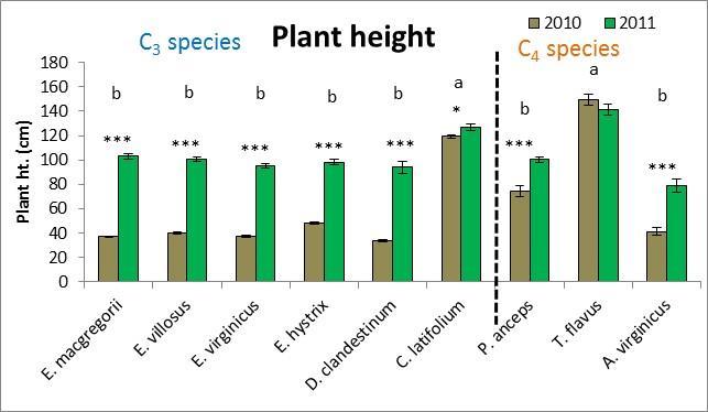
51 43

52 Figure 2.3: Drought effects for the Performance trait (ANPP) and macroscopic traits measured at the time of peak biomass. The species are listed on the x-axis in order of their flowering time with mean (± 1 SE). The left panel of graphs are species meansg (± SE) for each year (2010= dry year and 2011= wet year). The letter indicate significant differences between species with both years combined (p<.05). The asterisks above the bars indicate a significant difference between the years for a species (* p<.05, ** p<.001. *** p<.0001). The right panel of graphs shows the species means (± 1 SE) for plasticity or change in trait values between the two years (dry yr wet yr.) If the bar is above the line it had a higher value in the dry year. If the bar is below the line it had a higher value in the wet year. Different letters represent significant differences between species means (P value 0.05) determined by adhoc Tukeys. 44

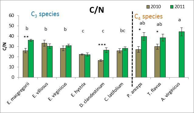
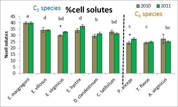
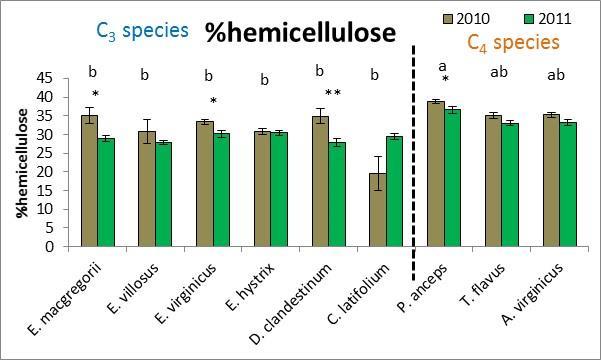
53 45

54 Figure 2.4: Drought effects for microscopic trait graphs for drought effects measured at the time of peak biomass. The species are listed on the x-axis in order of their flowering time with mean (± 1 SE). The left panel of graphs show species averages (± SE) for each year (2010= dry year and 2011= wet year). The letter indicate significant differences (p<.05) between species with both years combined. The asterisks above the bars indicate a significant difference between the years for a species (* p<.05, ** p<.001. *** p<.0001). The right panel of graphs shows the species means (± 1 SE) for plasticity or change in trait values between the two years (dry yr wet yr.) If the bar is above the line it did better in the dry year. If the bar is below the line it did better in the wet year. Different letters represent significant differences between species means (p<0.05) determined by adhoc Tukeys. 46

55 Figure 2.5: PCA drought results including all plasticity traits, macroscopic plasticity traits, and microscopic plasticity traits. Plasticity trait values are dry year- wet year. The circles indicate the species means that are not significantly different in pairwise comparisons using MRPP (p<.025). The percent of variance explained for each axis is in parenthesis beside the axis. 47

56 Figure 2.6: PCA results for competitive effects including all species, all traits, mono vs mixture treatments, and both years. All species means were significantly different determined by pairwise comparisons using MRPP (p<.025). The percent of variance explained for each axis is in parenthesis beside the axis. 48

57 Figure 2.7: Performance and Macroscopic trait graphs for differences in competitive ability between the two years (2010= dry year and 2011= wet year). The left side is the species means raw data and the right side is difference in competitive ability (Avg. mixture monoculture) for the two years. If the bar is positive, it did better in the mixture treatment than the monoculture. If the bar is negative, it did better in the monoculture. The bigger the bar, the bigger difference there was between Average mixture and the monoculture. Error bars are ±1std error. (* p<.05, ** p<.001. *** p<

58 Figure 2.8: Microscopic trait graphs for differences in competitive ability between the two years (2010= dry year and 2011= wet year). The left side is the raw data and the right side is difference in competitive ability (Avg. mixture monoculture) for the two years. If the bar is positive, it did better in the mixture treatment than the monoculture. If the bar is negative, it did better in the monoculture. The bigger the bar, the bigger difference there was between Average mixture and the monoculture. Error bars are ±1std error. (* p<.05, ** p<.001. *** p<

59 Figure 2.9: Competition and drought PCA results for each species comparing treatment means for all traits. The circles indicate the species means that are not significantly different in pairwise comparisons using MRPP (p<.025). The percent of variance explained is denoted in parenthesis for each axis. 51

60 Chapter 3: Differences in ecosystem properties between C 3 and C 4 grasses native to a historic North American Oak Savanna Abstract Since oak savannas of North America have been reduced to < 1 % of their historic ranges, restoration of these habitats are important to maintain the biodiversity and ecosystem functioning of these landscapes. Efforts to restore these oak savannas are hindered by the lack of dependable historic data describing these savannas before they were largely converted to other uses and by lack of restoration ecology guidelines for ecological restoration. To better understand the ecosystem dynamics of the herbaceous layer of a temperate oak savanna, a field monoculture experiment was performed to assess the ecosystem characteristics of six C 3 and three C 4 native bunchgrasses. This information can then be used to help predict how these species might function in a community setting, and to recommend ecological restoration guidelines to restore and maintain a functional grassland community assembly of the historic Bluegrass Oak Savanna-Woodland of Kentucky. This methodology can also be used in other savanna systems to better understand savanna grassland ecosystem functioning. The monoculture experiment included nine native bunchgrass species that were replicated 10 times to produce 90-2 meter 2 plots in a completely randomized design. The three experiments included in this study are: 1) plant characteristics were measured at peak biomass for each species, 2) a litter decomposition experiment was performed over 15 months, 3) a resin nitrate (NO 3- ) and ammonium (NH 4+ ) bag experiment was performed during the growing season of 2010, and 4) a soil nutrient study was performed in 2008 and again in The goal of this study was to measure the plant traits of these species and determine if the species were fast N cycling or slow N cycling species. The C 3 species were predicted to be fast N cycling species as they were thought to be found in more mesic eutrophic soils where N is less likely to be limiting. The C 4 species were predicted to be slow N cycling species as they were thought to be found in more nutrient poor and disturbed sites where N is more likely to be limiting. My results found that only C 3 species had trait values that promoted fast N cycling, but both C 3 and C 4 species had traits values that promoted slow N cycling. I concluded that N is not limiting in this experiment because: 1) decomposition of species with low quality litter was not hindered, 2) retention of N was found in the litter bags for all species, and 3) resin NO 3 -N and NH 4 -N levels were similar for species that were predicted to promote both mineralization and immobilization. Soil nutrient studies supported these observations as the nine species were not found to differentially deplete soil N levels. These findings do not support the resource-competition theory which is dependent upon N limitation. The results of this study suggests that other factors such as fire or grazing may have bigger impacts on the community setting of these grasses than competition for limiting N. 52

61 Introduction Savannas are grassland ecosystems characterized by the trees being sufficiently small or widely spaced so that the tree canopy is not closed (McPherson 1997) and are influenced by fire, climate, topography and soil (Nuzzo 1986). Savannas constitute 20 % of the Earth s land area and can be divided into tropical and temperate groups. Tropical savannas cover 15 % of the Earth s land area, are generally well represented in the scientific literature, and are extensive in Africa, Australia, and S. America (McPherson 1997). While temperate savannas of North America were historically common at the time of European settlement, most of these landscapes have been reduced to less than 1 % of their original area, are considered to be endangered landscapes (Anderson, Fralish et al. 1999), and are identified as critical areas for preservation (Klopatek, Olson et al. 1979). Furthermore, temperate savannas are not as well studied or represented in the scientific literature as tropical savannas(mcpherson 1997, Anderson, Fralish et al. 1999). Some potential reasons for this difference in the level of research activity are the absence of a professional discipline associated with savannas, limited understanding of the role and importance of savannas in temperate regions, and inconsistent definitions and/or interpretations of the term savanna (McPherson 1997). Thus, there is a lack of knowledge of the ecological relationships and ecological management practices for temperate savannas compared to adjacent forest, desert, or grassland landscapes (McPherson 1997). With European settlement in the eighteenth century, Midwestern Oak savannas in the USA all but disappeared within 20 to 40 years due to fire cessation and conversion of land to agricultural or urban development (Nuzzo 1986, Anderson, Fralish et al. 1999). The fact that only 2 % of Midwest Oak Savannas remained by 1986 (Nuzzo 1986) has caused this habitat to be listed as a globally imperiled ecosystem (Heikens and Robertson 1994). Conservation and restoration efforts of oak savannas are difficult due to: 1) the limited amount of historical data which was recorded mainly by European pioneers and land surveyors, and the unknown validity and motivation for these records (Nuzzo 1986), and 2) lack of restoration ecology studies to guide ecological restoration practices in the field (McPherson 1997). Benefits to restoring these historic landscapes include an increase in biodiversity and restoration of ecosystem functioning (McPherson 1997). Ecosystem functioning is influenced by climate, topography, nature of parent material, living organisms, and time (Brady 1990). Ecosystem functioning of oak savannas is further influenced by the more interactive factors such as fire, grazing, biogeochemical processes, and biotic interactions (Chapin, Matson et al. 2002). Savanna grasses can impact ecosystem functioning through positive or negative feedback loops that can influence fire or grazing frequencies, nutrient cycling, and soil nutrient availability (Bardgett, Mawdsley et al. 1999, Knops, Bradley et al. 2002). 53

62 Wei et al. (2013) characterized soil C and N stoichiometry is a main driver of ecosystem functioning of temperate grasslands in part because N is found to be a primary limiting nutrient in many grasslands (Polley and Detling 1988, Schlesinger 1991, Vitousek and Howarth 1991). Nitrogen is cycled through the plant, soil, and microbial communities and is intricately linked to the C cycle (Knops, Bradley et al. 2002, Wei, Yu et al. 2013). Plant species take up available N from the soil, produce biomass which eventually decomposes and returns the C and N back to the soil. Soil microbes regulate mineralization and mobilization rates of N in part by the amount of N in soil organic matter, and the quantity and quality of C and N of decomposing plant organic matter. Mineralization and immobilization of N by the soil microbes in turn determines the amount N that is available for plant uptake. Plant species differ in the amount and quality of biomass and litter they produce, N uptake rates, and the efficiency with which they use N (Wedin and Tilman 1990, Knops, Bradley et al. 2002, Jiang, Han et al. 2011). These species differences can result in positive or negative feedback loops (Vitousek 1982). A positive feedback loop is the result of a plant species that produces a low C:N biomass with high percent N and a low percent C particularly low in the recalcitrant forms of lignin and cellulose. This low C:N biomass produces a high quality litter that is then easily decomposed by the soil microbes. When soil microbes are not limited by N, mineralization occurs which coverts organic N to plant available inorganic N that is optimized under warm, moist soil conditions (McClellan, Deenik et al. 2007). Thus, fast N cycling species cycle nitrogen more rapidly through the plant, litter, and soil, and promotes plant available N. Similarly, a plant species that produces a high C:N biomass with low percent N and a high percentage of C particularly recalcitrant C. This high C:N biomass produces a low quality litter that is N limited that promotes immobilization. Immobilization is the process whereby soil microbes use inorganic N to break down the N limited litter that can ultimately result in soil N deficiencies and limit plant N availability (McClellan, Deenik et al. 2007). Thus, slow N cycling species cycle less nitrogen more slowly through the plant litter and soil which limits plant available N. Also since lignin in the litter turns into humic substances in soil organic matter, litter with high amounts of lignin leads to higher soil organic C and N pools (De Deyn, Cornelissen et al. 2008). Moreover, slow N cycling plants should be selected for when water or nutrients are limiting plant growth. Thus, N limitation creates a positive feedback that results in slower C cycling and an increase of soil organic C and N (De Deyn, Cornelissen et al. 2008). N cycling is also influenced by a plants ability to retranslocate N from dying aboveground biomass to belowground parts, and synchronizing the seasonality of plant activity with precipitation. Grass species are known to vary in their ability of retranslocate N from dying aboveground biomass to crowns and roots (Norris and Reich 2009). Retranslocation of N is thought to be favored in N limited 54

63 environments where the conservation of N is important, and less important in more mesic environments where soil N may not limiting (Norris and Reich 2009). The retranslocation of N increases the C:N of the litter and promotes immobilization which in turn further limits plant available N. Moreover, plant uptake of N is also dependent on water availability as uptake of nitrate (NO 3- ) and ammonium (NH 4+ ) happens in the root hairs and is dependent on water. Plants that temporally synchronize N uptake at the time they are most actively growing with seasonal precipitation can show an increase of % tissue N. This would lower C:N of litter and promote mineralization and increase plant available N. Plants that do not synchronize plant N uptake with precipitation could experience decreased plant N availability and uptake, and possibly the accumulation of nitrates in the soil that then becomes susceptible to leaching (McCulley, Burke et al. 2009). While these positive and negative feedback loops can have effects at the ecosystem scale, plant available N also differs at more local scales that can select for fast or slow N cycling species. This local scale can have major impacts on the spatial distribution of species in a community. At the ecosystem level, the resource-competition theory predicts that in N limited environments, the species that conserves N and most efficiently reduces soil N availability will have a competitive advantage over neighboring species that have higher N demands (Fargione and Tilman 2006). In N limiting conditions, slow N cycling species are predicted be better competitors than fast N cycling species which would result in increased production and abundance of slow N cycling species in the community (Fargione and Tilman 2006). However if N is not limiting, faster cycling N species should be at a competitive advantage which would result in their increased production and abundance in the community. At more local scales, fast N cycling species would persist on more fertile sites, and slow N species would persist on less fertile and more disturbed sites. The purpose of this study is to test these theories using six C 3 grasses and three C 4 perennial bunchgrasses to help predict a functional grassland community setting as part of the ecological restoration of the historic Oak Savanna-Woodland located in the Inner Bluegrass Region of Kentucky. U.S.A. The Bluegrass Savanna-Woodland was considered by Braun (1943) to be anomalous or unexpected in the middle of the mixed mesophytic forest biome. Wharton and Barbour (1991) characterized this area as a savanna-woodland with an open forest dominated by trees but retaining a well-developed grassy undergrowth. This savanna-woodland was best described at the time of European settlement in the mid to late 1700 s as having rolling topography that is mildly karst, a highly phosphatic Ordovician Limestone parent material that produces a silt loam soil that is fertile, deep, and well drained, vast cane breaks (Arundinaria gigantea), large mature trees including Oak (Quercus) and Ash (Fraxinus), and a C 3 graminoid dominated herbaceous layer (McInteer 1952, Wharton and Barbour 1991, Campbell 2004). 55

64 With European settlement, native grasses were rapidly replaced by non-native C 3 forage grasses (Festuca arundinacea, and Poa pretensis) so that no intact savanna grassland remains in this region (Bryant, Wharton et al. 1980). The C 3 grasses were thought to be dominant in both abundance and number of species where they frequented the woodlands (Wharton and Barbour 1991) with mesic eutrophic soils as well as the more open woods (Campbell 2004). The C 4 grasses were predicted to be fewer in the number of species and found in local openings on poorer soils or openings created by disturbance such as fire or bison trails (Campbell 2004). These nine grasses were grown in a monoculture experiment to assess the plant traits associated with N and C cycling of each species individually. I hypothesized that: 1) The C 3 grasses will promote fast N cycling, and C 4 grasses will promote more conservative or slow N cycling. 2) If N is limiting at the ecosystem level, fast N cycling species should deplete soil N less than slow N cycling species according to the resource-competition theory. Results of this experiment can be used to better understand the dynamics of this savannawoodland and how these nine species would function in a community. This study also uses methodology that could be used in other savanna landscapes that could guide ecological restoration efforts of these endangered oak savanna landscapes. Materials and Methods Study Site The experiment was conducted in a relatively flat, tall fescue (Festuca arundinacea) dominated abandoned paddock located at Griffith Woods Wildlife Management Area (WMA). Griffith Woods WMA is considered to be the best Bluegrass Savanna-Woodland remnant in the Inner Bluegrass Region of Kentucky. It includes 746 acres in southern Harrison County, Kentucky (Latitude N , Longitude W ) and lies on the northern edge of the Inner Bluegrass Region of Kentucky. While the vegetation of Griffith Woods WMA is known for its remnant Blue Ash-Oak savanna-woodland with year old trees of Fraxinus quadrangulata (Blue Ash), Quercus macrocarpa (Burr Oak), Quercus muhlenbergii (Chinquapin Oak), and Quercus shumardii (Shumard Oak), the herbaceous layer is dominated by non-native C 3 forage grasses (Festuca arundinacea, and Poa pretensis). While there is a long history of human occupation and agricultural use (Wharton and Barbour 1991), one management goal was to restore a portion of the property back to pre-european settlement savanna woodland vegetation. Ecological restoration efforts include native tree planting, native cane planting (Arundinaria gigantea), and invasive species removal. 56

65 The Inner Bluegrass Region of Kentucky encompasses about 2,400 square miles and is underlain by Ordovician Limestone which was pushed up over the millennia by the Jessamine Dome of the Cincinnati Arch that has produces a mildly karst rolling topography (Wharton and Barbour 1991). This highly phosphatic limestone produces a silt loam soil that is fertile, deep, and well drained (Wharton and Barbour 1991). The warm, temperate, and humid climate is continental and highly variable (Wharton and Barbour 1991). Average yearly precipitation for the Bluegrass Region is 112 cm/year with typical wet springs and dry autumns (Wharton and Barbour 1991). On Average the growing season is 181 days with average annual temperature of 13 Celsius with generally mild winters and hot summers (Wharton and Barbour 1991). Species The nine native bunchgrasses (Wharton and Barbour 1991, Campbell 2004) included in this study are listed in Table 3.2.1in the order of their flowering times. The nine species are categorized in two functional groups C 3 (or cool season) grasses and C 4 (or warm season) grasses. The six C 3 grasses included in this study are associated with wooded habitats, and the three C 4 species are associated with more open habitats (Wharton and Barbour 1991, Campbell 2004). Four of the C 3 grasses are Elymus species or wildryes. The Elymus species are well documented in historical records and are thought to have been abundant at the time of European settlement in the mid to late 1700 s (Wharton and Barbour 1991). Elymus virginicus is common in open woods, thickets and old fields, and Elymus villosus is frequent in dry and moist open woods (Wharton and Barbour 1991). Elymus macgregorii can be confused with E. virginicus but flowers a month earlier and is also found in woods and thickets (Committee 2002), and Elymus hystrix is frequent in the woods (Wharton and Barbour 1991). The Elymus species have a different life history pattern with significant niche differentiation from the other species. They flower in the spring or early summer, set seed, and then go dormant during the hottest months of the summer. They regrow tillers in the fall which overwinter and produce flowering culms the next spring. Dichantheilium clandestinum may have been referred to as buffalos grass in historical records where it is frequent in open woods, thickets, and fencerows, especially on low ground (Wharton and Barbour 1991). D. clandestinum also has life history traits that differ from the other species in this study. D. clandestinum first produces cleistogamous flowering culms, and then later in the season they produce self-fertilizing chasmogamous flowers on small inflorescences that are usually hidden within the sheathes. Both types of flowers produce viable seeds. While this species did not produce a lot of tillers, it had the greatest ability for tiller branching, so one tiller could be quite large and heavy. Clandestinum latifolium is frequent on wooded stream banks, on floodplains, and in other moist habitats (Wharton and Barbour 1991). C. latifolium is also used for in horticultural plantings and can be known to be quite invasive. 57

66 The three C 4 species are generally found in more open sites. P. anceps is found less commonly and on moist ground, and T. flavus is common in old fields, woodland borders, open woods, pastures, and roadsides (Wharton and Barbour 1991). Andropogon virginicus is common in old fields and overgrazed pastures (Wharton and Barbour 1991). A. virginicus grew really well the first year it was planted, but did successively worse each year. Experimental procedures Seeds for each species were collected in the Bluegrass Region of Kentucky and cold (wet) stratification requirements were determined through the seed testing laboratory at the Regulatory Services at the University of Kentucky. The stratified seeds were germinated in a heated greenhouse on a flooding table in 72 hole plant trays filled with Pro-Mix potting soil. These plugs were planted in the field plots at 169 plugs/2 meter 2 plot with a hand trowel to minimize disturbance. In a completely randomized design, nine native bunchgrass species monocultures plus one species mixture treatment were each replicated 10 times to produce meter 2 plots. The species mixture treatment was not included in this analysis. Initial preparation of the field site included mowing after which the grass clippings were raked into piles and burned. The field was then sprayed with Roundup herbicide at recommended concentrations to kill all the vegetation. A second application of Roundup was applied to areas that did not die back after the initial Roundup treatment. The plots were watered as needed with a garden hose after initial planting, and rainfall was recorded at the site. The C 3 species were planted in March through May, and the C 4 species were planted in June and July. The first field season (2008) Elymus virginicus, Elymus villosus, Elymus mcgregorii, Panicum anceps, Tridens flavus, and Andropogon virginicus were planted with the remaining species planted the second growing season (2009). An 18 inch path was maintained around each of the plots by mowing. The experiment and the surrounding area were maintained by hand weeding, spot spraying with Roundup, and mowing. In 2010 the net primary production N content data was collected and the inorganic nitrogen plant availability study was performed. There was little variation in monthly average temperatures between 2010 (Kentucky Mesonet), and the (1895 to 2013) long term average of the Bluegrass Region (NOAA/ESRL (Figure 3.3b). There was significant precipitation variation between 2010 which was a relatively dry year (Kentucky Mesonet), compared to the (1895 to 2013) long term monthly precipitation average for the Bluegrass Region (Figure 3.3a). The year 2010 witnessed a 15% decrease in annual precipitation primarily in January to March and August to October compared to the Bluegrass Region long term average (Figure 3.6a). 58

67 Soil analysis The soils at the site are well drained uplands of Faywood silty clay loam according to Web Soil Survey maintained by the Natural Resources Conservation Service (NRCS). Available water capacity is low (about 12cm) and it is considered not prime farmland. Soil horizons are: 0 to 15 cm: silty clay loam, 15 to 76 cm: clay, 76 to 86 cm: and unweathered bedrock. The soil for this site was a silt loam with an average of 17% sand (range ), 68% silt (range ) and 14% clay (range ). The other soil parameters for this site that were assessed at the initiation of the study are shown in Table 3.2. Site level data were collected in October 2008, soil cores were taken in the top 10 cm of each plot. Those samples were pooled and mixed thoroughly by species and the species mixture treatment to create one sample for each species and the species mixture treatment. Initial assessments of cation exchange capacity (CEC), base saturation, soil texture class, and water holding capacity were performed on these (Table 3.2). Bulk density samples were collected in October 2012 with a replication of 5 for each species plus the species mixture treatment. Since bulk density was not measured at the beginning of the experiment (2008), control soil cores were collected in 2012 in relatively undisturbed spots around the perimeter of the experiment as a proxy for initial conditions. Soil nutrient concentrations were converted to pool sizes using the bulk density. Additional soil cores for each plot were collected in October 2008 and October For individual plot samples, the Mehlich 3 test was performed by Regulatory Services at the University of Kentucky to determine soil levels of phosphorous, potassium, calcium, magnesium, zinc, ph and buffer ph. Total % soil carbon and % soil nitrogen also were determined by Regulatory Services at the University of Kentucky using the Elementar vario MAX CNS Analyzer. Net primary production N content Due to the large seasonal variation of flowering times of the nine grass species, aboveground net primary production (ANPP) values were taken for each species at peak biomass (or time of flowering) and ranged from May to September (Table 3.1). A 15 cm 2 area was randomly chosen for each plot where aboveground biomass 5 cm above soil level was clipped, dried, and weighed. Total organic carbon and total organic nitrogen concentrations in plant biomass were measured using the Elementar vario MAX CNS Analyzer by the soil testing laboratory of the Regulatory Services at the University of Kentucky. The acid-fiber digest procedure was used to determine cellulose and lignin concentrations of the 2010 peak biomass samples using the Ankom 200 Fiber Analyzer according to the procedures found at under the procedures tab. ANPP-N was calculated by multiplying ANPP times the %total tissue Nitrogen and Nitrogen Use Efficiency (NUE) was calculated as 1/%tissue Nitrogen (Table 3.6). 59

68 Inorganic Nitrogen Resin Study Plant available inorganic nitrogen was measured for 7 months over the growing season (March through October) in 2010 using resin bags that absorb both ammonium (NH 4+ ) and nitrate (NO 3- ) ions. Resin bags were constructed using a nylon mesh bag filled with a mixture of 7.4 milliliter of a cation and 7.4 milliliter of an anion exchange resin. The bags were knotted on each end and a neon orange fishing line was attached to the bag for easy retrieval from the plots. For each plot, a resin bag was flatly placed 5 centimeters below the soil surface in April The bags were collected and replaced each month throughout the growing season until October Seven monthly pickups of 100 plots per pickup resulted in 700 resin bags analyzed. Using the KCl extraction technique, one resin bag was placed in 50 mls of 2N KCl, and the extractants were analyzed colorimetrically for NO3-N and NH4-N using a Bran- Luebbe auto-analyzer. Nitrates were analyzed using the hydrazine sulfate - copper sulfate reduction method and ammonium was analyzed using the sodium nitroprusside phenol method. Litter decomposition To assess litter decomposition rates for each species, 5 grams of standing dead dried leaves and stems were collected in the Autumn of 2009, clipped to ~2 cm long pieces, and sealed into 10 x 10 cm 2 bags made of fiberglass-nylon mesh with 1.4 mm 2 openings. The bags were sealed with a TISH-200 impulse sealer and secured to the soil surface with metal ground staples. The bags were set out in replicates with one replicate consisting of one litter bag for each species or nine bags. At each pickup time four replicates (or 36 bags) were picked up. There were six pickup times and four replicates picked up, resulting in 216 litterbags in total. When the samples were picked up, they were oven dried at 55º C and weighed. They then were ground using a coffee grinder and sent to the soils laboratory at Regulatory Services to be analyzed for total % nitrogen and total % carbon using the Elementar vario MAX CNS Analyzer. Each sample was adjusted for ash free weight by burning ~0.5 grams of a sample in a muffle oven for 5 hours at 525 C and then in a drying oven for 2 hours at 105 C. That weight was recorded and divided by the sample weight to get the % ash of the sample. The % ash was deducted from the total litter weight to get the ash free weight of the whole sample. The bags were set out in January 25, 2010 in a flat area adjacent to the monoculture experiment. The first five pick-up dates were at 2 month intervals from March to November The last set of replicates was picked up in June 20, 2011 with a 7 month interval. Statistics The statistical program PAST (Hammer 2001) was used to normalize the data and each ANOVA was performed in SAS (9.3: SAS Institute, Cary, NorthCarolina, USA) using PROC MIXED (SAS 2010). Multivariate analysis was performed in the program PC-ORD (6.08: MjM Software, Gleneden Beach, Oregon, U.S.A.) using Principle Components Analysis (PCA) using the Euclidean distance measurement 60

69 (McCune and Mefford 2011). The data was not standardized and all response variable were included in the analysis. The Euclidean distance measurement was also used with Multi-Response Permutation Procedures (MRPP) within PC-ORD to discern significant species effects. Repeated measures analysis was performed in SAS (9.3: SAS Institute, Cary, NorthCarolina, USA) using PROC MIXED for the resin data and the litter decomposition data. For the resin data, a repeated measures model was run for NH 4 -N and NO 3 -N including species and time effects, and also a repeated measures model was run for each species which looked at time effects. Results Species characteristics While significant species differences were found for every species characteristic (Figure 3.2), there was no clear pattern between C 3 and C 4 species. Plant traits that promote fast N cycling include high amounts of N, low NUE, low amounts of C and recalcitrant C, and plants that do not retranslocate significant amount of N to crowns and roots. Plant traits that promote slow N cycling include low amounts of N, high NUE, high amounts of C and recalcitrant C, and plants that are effective at retranslocating N to crowns and roots. To characterize the nine species as promoting either fast N cycling or slow N cycling, I compared significant differences between species for each plant trait. E. macgregorii had the most traits that promoted fast N cycling (Figure 3.2). While E. macgregorii did not have high amounts of N, it did have low amounts of recalcitrant C and was not effective at retranslocating N. E. hystrix and D. clandestinum had plant trait values that promoted both fast and slow N cycling. E. hystrix had high ANPP, low C:N and low recalcitrant C which promotes fast cycling, but also had high lignin:n, low levels of tissue N, high levels of lignin that promotes slow N cycling. Also, E. hystrix was effective at retranslocating N. The fast N cycling traits for D. clandestinum were low C:N, high % tissue N, and low NUE, and the slow N cycling traits were a high percent of cellulose and lignin. D. clandestinum was significantly better than all the other species at retranslocating N. The other six species had more plant trait values that promoted slow N cycling compared to fast N cycling. E. villosus and E. virginicus generally had the same species characteristics with high lignin:n, low % tissue N, high % lignin, and high NUE that promoted slow N cycling. E. villosus and E. virginicus were not effective at retranslocating N. For C. latifolium and T. flavus, high ANPP-N was the only trait that promoted fast N cycling. Slow N cycling plant traits for C. latifolium and T. flavus were low % tissue N, high NUE, and high % cellulose. T. flavus also had a high lignin:n and high amounts of recalcitrant C. P. anceps was the only species to have just slow N cycling traits with low % tissue N, high NUE, high % cellulose, and was effective at retranslocating N. In conclusion, I found that three C 3 species, (E. macgregorii, E. hystrix, and D. 61

70 clandestinum) had the most number of plant traits that promoted fast N cycling, and the other six species had more plant traits that promoted slow N cycling. Litter Decomposition Significant species differences were found for initial litter quality, litter decomposition rate (k value) and C:N at the last pickup date (Figure 3.3). Litter decomposition characteristics that promote fast N cycling are low C:N, high N content, low C content, and a fast litter decomposition rate. Litter decomposition characteristics that promote slow N cycling are high C:N, low N content, high C content, and a slow litter decomposition rate. To characterize the nine species as having either fast N cycling or slow N cycling litter, I compared significant differences between species for each litter characteristic. In general I found that the litter characteristics of the C 3 species promoted fast N cycling, and the litter characteristics of the C 4 species promoted slow N cycling. E. villosus and E. virginicus had the most definite litter characteristics that promoted fast N cycling. E. villosus and E. virginicus had the highest initial quality litter compared to the other seven species with significantly higher % litter N, and significantly lower litter C:N (Figure 3.3). Also, the litter of E. villosus decomposed the fastest, and E. virginicus had the lowest litter C:N at the last litter bag pickup (Figure 3.3B and C). The litter of E. macgregorri and D. clandetinum promoted fast N cycling with a relatively higher % litter N (Figure 3.3). The only C 3 species that promoted slow N cycling was E. hystrix that had a high litter C:N. Significant litter characteristics of the three C 4 species promoted only slow N cycling. A. virginicus had the most litter characteristics that promoted slow N cycling with low % litter N, and a high litter C:N. A. virginicus also had the slowest decomposition rate and the highest litter C:N at the last litter bag pickup date (Figure 3.3). Litter characteristics of P. anceps were similar to A. virginicus except that P. anceps had a faster litter decomposition rate (Figure 3.3). The high litter C:N of T. flavus promoted slow N cycling (Figure 3.3). The ANOVA repeated measures analysis for the litter decomposition experiment had significant species effects, time (days incubated) effects, and species x time effects for all response variables listed in Table 3.4 except that % C did not have a significant species x time interaction. Therefore, % C tended to decline through time for all species. Since a significant interaction term was detected for all variables except for %C, a one way ANOVA was performed for each species. All species had a significant time effect for all variables listed in Table 3.4 except that C. latifolium, P. anceps, and T. flavus did not have a significant time effect for litter N. Therefore, the amount of N in the litter for C. latifolium, P. anceps, and T. flavus did not significantly change over the course of this experiment. 62

71 Litter C concentration, % of initial amount remaining, and total amount tended to decline the over the course of the experiment for all species (Figure 3.5). However, litter N was variable over the course of the experiment and between species in both concentration and % of initial amount remaining (Figure 3.5). The variation in % N resulted in a relatively constant total amount of N over the course of the experiment and for all species (Figure 3.5). Thus, the litter was losing mass and C but retaining N. E. villosus and E. virginicus had a high amount of N in initial litter, but that N was quickly lost within the first 60 days of incubation (Figure 3.5). Also, E. villosus and E. virginicus were the only species to lower % N below initial % N levels (Figure 3.5). All other species maintained or increased % N during the course of the experiment (Figure 3.5). The C 4 species, C. latifolium and E. hystrix increased % N by 50 % or more by the end of the experiment (Figure 3.5). Patterns of total litter N (% N x litter wt.) and C (% C x litter wt.) from January 2010 to June 2011 for each species are shown in Figure 3.6. Since total amounts of litter N and C were graphed, litter C generally declines and litter N remains relatively constant over the course of the experiment. E. villosus, E. virginicus, and E. hystrix, had significantly lower amounts of litter N after the first 60 days, and then relatively constant litter N amounts for the rest of the experiment. D. clandestinum also had a drop in litter N in the first 60 days, but then increased litter N over the course of the growing season. All species except for P. anceps generally lose carbon until July which is the beginning of the drought and temperatures are at the maximum (Figure 3.6). P. anceps continues to reduce C into September which is at the peak of the drought. D. clandestinum and P. anceps reduced litter C the slowest with D. clandestinum retaining the most litter C over the first five intervals (until October). Nitrate and ammonium resin data Significant species differences were found for NO 3 -N, NH 4 -N, total resin N, N soil pools, C soil pools, and bulk density (Figure 3.7). I predicted that fast cycling N species with high litter N and low litter C:N should decompose more rapidly and promote mineralization. Mineralization occurs when litter C:N is less than 20:1 (Namuth 2014). Initial litter C:N of E. villosus and E. virginicus had the lowest litter C:N (avg and respectively) followed by D. clandestinum (avg ), E. macgregorii (avg ) (Table 3.3). A fast cycling N species should then be adapted to quickly take up plant available N. I predicted that slow cycling N species with low litter N and high litter C:N should decompose more slowly and promote immobilization. Immobilization occurs when litter C:N is greater than 20:1 (Namuth 2014). Initial litter C:N of P. anceps was the highest (avg ) followed by A. virginicus (avg ), T. flavus, E. hystrix, and C. latifolium (Table 3.3). Immobilization limits plant available N and can lower soil N. Since well decomposed litter has a C:N of around 10:1 (Namuth 2014), all nine species were relatively well decomposed at the end of 528 days of incubation with P. anceps 63

72 (avg ) and A. virginicus (avg ) the least decomposed (Table 3.3). However, by the end of the experiment E. villosus and E. virginicus lowered litter C:N by 35% and 30% respectively, while A. virginicus, P. anceps, T. flavus and E. hystrix lowered C:N by at least 70 % (Table 3.3). This suggests that N was not limiting litter decomposition for the species with high initial litter C:N. Also, species that had higher % lignin were predicted to have high C and N soil pool levels which should then lower bulk density. I did not find a noteworthy positive correlation between % lignin (Figure 3.2) and N and C soil pools, and bulk density (Figure 3.2) but E. virginicus, E. hystrix, D. clandestinum, C. latifolium, and T.flavus did show the general trend. Uptake of plant available N is optimal if it is synced with seasonal precipitation. Since only the amount of resin NO 3 -N and NH 4 -N was measured for each species, plant available N and the amount of N that was taken up by the plant could not be teased apart. For this instance, I will assume that there was more plant available N for E. macgregorii, E. villosus, E. virginicus, and D. clandestinum which were the species with high quality litter. Of these four species, E. virginicus and D. clandestinum were the only two species that efficiently depleted both NO 3 -N and NH 4 -N throughout the growing season (Figure 8). Although E. villosus had the highest litter quality and decomposed the fastest (Figure 3.3), it was able to efficiently deplete NH 4 -N but not NO 3 -N (Figure 3.7 and 2.8). The peak in NO 3 -N coincides with the time E. villosus goes dormant, and also the time the nitrifying bacteria may be most active (McClellan, Deenik et al. 2007). Resin bag levels for E. macgregorii were similar to E. villosus, E. virginicus but E. macgregorii did not deplete NH 4 -N as efficiently as E. villosus. The assumption that there was less plant available N for the species that had low litter quality does not hold true for my data. E. hystrix, P. anceps, T. flavus, and A. virginicus had low quality litter but did not have low levels resin NO 3 -N and NH 4 -N (Figures 2.7 and 2.8). In fact E. hystrix, P. anceps, and A. virginicus had the highest levels of total resin N (Figure 3.7). Since these four species had higher levels of resin N, I have to assume that plant available N is similar between the species and that my resin data may be a better measurement of plant uptake. If this is true, the four species with low quality litter (E. hystrix, P. anceps, T. flavus, and A. virginicus) were less efficient at N uptake than the four species with high quality litter (E. macgregorii, E. villosus, E, virginicus, and D. clandestinum). Significant species, time, and species x time effects were found in the repeated measures analysis for resin NO 3 -N and NH 4 -N (Table 3.5). Since the species x time interaction was significant, a separate repeated measures was performed for each species. For NO 3 -N, all species had a significant time effect, and all species except for E. villosus had a significant time effect for NH 4-N (Table 3.5). In general, NO 3- N levels varied more over the growing season than NH 4 -N levels (Figures 2.7 and 2.8). All species 64

73 except for E. virginicus, D. clandestimnum, and T. flavus showed a significant increase in resin NO 3 -N in July (Figure 3.8) when the monthly temperature average was the highest for the year (~25º C) and precipitation fell below the long term average for the Bluegrass Region of Kentucky (Figure 12.). This July spike also coincides with the time the nitrifying bacteria may have been most active which may account for the drop in resin NH 4 -N for E. macgregorii and C. latifolium (Figure 3.8). The late summer drought that lasted from July to October and was most severe in September (Figure 3.1) which coincides with the increased NO 3 -N levels for E. villosus and E. hystrix even though these two species were dormant during the beginning of this drought. Even though the four Elymus species were dormant during the month of July, resin NH 4 -N levels remained relatively constant. Soil data At the beginning of the experiment in October 2008, significant species differences were found for phosphorous, potassium, magnesium, and ph (Figure 3.9). The only significant adhoc tukeys species pairwise comparisons were found for magnesium and ph (Figure 3.9). At the end of the experiment in October 2012, no significant species effects were found for any of the soil nutrients or ph (Figure 3.9). Comparing all species and both years (2012 and 2008), significant species effects and year effects were found for ph (spec p =.012, year p<.0001), phosphorous (spec p =.002, year p=.05), potassium (spec p<.0001, year p<.0001), calcium (spec p =.0002, year p<.0001), and magnesium (spec p =.012, year p<.0001). No significant species x year interactions were detected. Soil ph, and levels of potassium, calcium, and magnesium were lower in 2012, and soil levels for phosphorous were higher in To determine if the species had differing effects on soil nutrients, an ANOVA analysis was performed that analyzed the amount of change between the 2 years ( ). Only ph was found to have significant species effects where E. hystrix lowered ph significantly more than T. flavus (Figure 3.9). To test if the species significantly varied in multivariate space, the differences between the two years for all soil nutrients were plotted using principle components analysis (PCA). The PCA graph was sorted by species and a multi-response Permutation Procedures (MRPP) was performed using Euclidean distances to test for significant pairwise differences between species. No significant species differences were detected (p=.604) using differences ( ) for all soil nutrients, ph and buffer ph. I also performed the same PCA analysis excluding ph and buffer ph with similar results. Discussion My first hypothesis was partially confirmed in that C 3 species had plant traits that promoted fast N cycling. My first hypothesis was also partially falsified because both C 3 and C 4 species had plant traits that promoted slow N cycling. Considering all the C 3 species, my hypothesis was supported by three Elymus species (E. macgregorii, E. villosus, and E. virginicus), partially supported for D. clandestinum, 65

74 and generally not supported for E. hystrix, and C. latifolium. E. virginicus had the most plant traits that supported the fast N cycling strategy with high quality litter that rapidly decomposed, and was efficient at taking up both NO 3 -N and NH 4 -N. After E. virginicus, E. villosus and E. macgregorii had the most plant traits that promoted fast N cycling except that E. villosus was less efficient at NO 3 -N uptake, and E. macgregorii had lower quality litter and was less efficient at taking up both NO 3 -N and NH 4 -N. D. clandestinum had traits that promoted both fast N cycling and slow N cycling. Traits that promoted fast N cycling were high litter N and efficiency at taking up both NO 3 -N and NH 4 -N. The slow N cycling traits of D. clandestinum were retranslocation of the most N to crowns and roots, and losing litter C the slowest compared to all the other species. My first hypothesis was supported by the C 4 species which had traits that promoted only slow N cycling. While all three C 4 species had low litter quality and were inefficient at taking up both NO 3 -N and NH 4 -N, the litter of A. virginicus decomposed the slowest, and P. anceps was better at retranslocating N, lost litter C the slowest, and was the least decomposed at the end of the experiment. C. latifolium and E. hystrix were the two C 3 species that tended to have slow N cycling traits with lower litter quality than the other C 3 species, and inefficient at taking up NO 3 -N. My data does not support the second prediction that slow N cycling species will have a positive feedback loop where poor litter quality will promote immobilization, and limit plant available N. For fast N cycling species as well as slow N cycling species, similar levels of resin NO 3 -N and NH 4 -N were observed. Also decomposition of litter was not limited by N as all species except for E. villosus and E. virginicus increased percent litter N over the course of the experiment. Thus, similar to other litter decomposition studies (Melillo, Aber et al. 1982, Hobbie 1996) the litter was losing mass and C but retaining N. Also species with initially high litter C:N reduced litter C:N by over 70 % over the course of the experiment which again suggests no N limitation. Knops et al. (2002) suggests that the negative slow N cycling feedback loop does not limit plant available N because species differences in litter quality have a limited impact on plant available N compared to the N in the soil organic pool which accounts for 90 % of total ecosystem N. Most N gained from the decomposing litter is retained and incorporated into the soil organic matter, which prevents immediate feedbacks to the plants. The soil organic matter has a bigger impact on mineralization and immobilization and ultimately plant available N compared to plant and litter characteristics (Knops, Bradley et al. 2002). At the ecosystem level, the soil data does not suggest that the species significantly affected soil parameters over the four years this experiment was conducted. Percent C and % N did not significantly differ for any species over the course of this experiment. Thus, these nine species did not differentially deplete soil N as was predicted by the resource-competition theory. All this data is evidence that N may not be the primary limiting nutrient for this savanna-woodland which is opposite of what has been found 66

75 to be true for many temperate grasslands (Polley and Detling 1988, Schlesinger 1991, Vitousek and Howarth 1991). Knops et al (2002) suggested that species differences in quantity and quality of litter did not have large impacts on N cycling but by plant species impacts on nitrogen inputs and losses. Furthermore other studies suggest that other factors besides plant and litter characteristics have a bigger impact on ecosystem N cycling such as the diversity and abundance of soil microbial communities, and disturbances such a fire and grazing (Reich, Grigal et al. 1997, Knops, Bradley et al. 2002). These results are consistent with the reported species distribution in the field. The fast N cycling species will have traits that make them better adapted for habitats that are not limited by N and water. The four fast N cycling C 3 species, E. macgregorii, E. villosus, E. virginicus and D. clandestinum do frequent the Bluegrass savanna-woodlands with mesic eutrophic soils as well as the more open woods (Wharton and Barbour 1991, Campbell 2004). The Elymus species may also be best adapted at taking up plant available N because the time they are actively growing and plant N demands are high, coincides with the Bluegrass Region s wet spring. Also, the Elymus species produce high quality litter during the summer months when soil microbes are most active. My data also supports the prediction that the slow N cycling species will be best adapted for N limited habitats. The C 4 grasses had more conservative N traits that promote slow N cycling which would explain why they are found in local openings on poorer soils in the Bluegrass savanna-woodland or openings created by disturbance such as fire or bison trails (Campbell 2004). The C 4 species actively grow during the summer months which was during the summer drought. The lack of soil water during the summer drought may have limited the uptake of inorganic N. Also, increased nitrifying bacteria activity during the summer months may partially explain the NO 3 -N peaks during the summer months which can be seen for most of the species (Figure 3.8). In conclusion, most C 3 species were found to have fast N cycling traits, and C 4 species were found to have slow N cycling traits that could explain their local distribution for the Bluegrass savannawoodland. Unlike many other temperate grassland systems, N limitation was not found to be a main determinant in sorting species in a community assembly. Other factors besides plant mediated competition for N may have bigger impacts on ecosystem N cycling in the savanna-woodland. Since savannas are dependent on disturbance, fire and grazing could have major impacts of N inputs and losses at the ecosystem level. Future restoration ecology studies to investigate the effect of fire and grazing on these savannas can provide more effective ecological restoration guidelines. Literature Cited Anderson, R. C., J. S. Fralish and J. M. Baskin, Eds. (1999). Savannas, Barrens, and Rock Outcrop Plant Communities of North America. Cambridge, UK, Cambridge University Press. 67

76 Bardgett, R. D., J. L. Mawdsley, S. Edwards, P. J. Hobbs, J. S. Rodwell and W. J. Davies (1999). "Plant species and nitrogen effects on soil biological properties of temperate upland grasslands." Functional Ecology 13(5): Brady, N. C. (1990). The Nature and Properties of Soils. New York, Macmillan Publishing Company. Braun, E. L. (1943). Deciduous Forests of Eastern North America. Philadelphia, Blakiston Co. Bryant, W. S., M. E. Wharton, W. H. Martin and J. B. Varner (1980). "The Blue Ash-Oak Savanna- Woodland, a Remnant of Presettlement Vegetation in the Inner Bluegrass of Kentucky." Castanea 45(3): Campbell, J. (2004). Comparitive Ecology of Warm-Season (C4) versus Cool-Season Grass (C3) Species in Kentucky, with Reference to Bluegrass Woodlands. 4th Eastern Native Grass Symposium University of Kentucky. Chapin, F., P. Matson and H. Mooney (2002). Princples of terrestrial ecosystem ecology. New York, Springer. Committee, F. o. N. A. E., Ed. (2002). Flora of North America: Magnoliophyta: Commelinidae (in part): Poaceae, part 1. New York, Oxford University Press. De Deyn, G. B., J. H. C. Cornelissen and R. D. Bardgett (2008). "Plant functional traits and soil carbon sequestration in contrasting biomes." Ecology Letters 11(5): Fargione, J. and D. Tilman (2006). "Plant species traits and capacity for resource reduction predict yield and abundance under competition in nitrogen-limited grassland." Functional Ecology 20(3): Hammer, Ø., Harper, D.A.T., Ryan, P.D. (2001). PAST: Paleontological statistics software package for education and data analysis. Palaeontologia Electronica P. Electronica. Heikens, A. L. and P. A. Robertson (1994). "Barrens of the Midwest: A review of the literature.." Castanea 59: Hobbie, S. E. (1996). "Temperature and plant species control over litter decomposition in Alaskan tundra." Ecological Monographs 66(4): Jiang, L. L., X. G. Han, N. Dong, Y. F. Wang and P. Kardol (2011). "Plant species effects on soil carbon and nitrogen dynamics in a temperate steppe of northern China." Plant and Soil 346(1-2): Klopatek, J. M., R. J. Olson, C. J. Emerson and J. L. Jones (1979). "Land -use confict with natural vegetation in the United States.." Environmental Conservation 6: Knops, J. M. H., K. L. Bradley and D. A. Wedin (2002). "Mechanisms of plant species impacts on ecosystem nitrogen cycling." Ecology Letters 5(3): McClellan, T., T. J. Deenik and S. t. P. (2007). "Soil Nutrient Managment for Maui County." Retrieved 2014, 2007, from 68

77 McCulley, R. L., I. C. Burke and W. K. Lauenroth (2009). "Conservation of nitrogen increases with precipitation across a major grassland gradient in the Central Great Plains of North America." Oecologia 159(3): McCune, B. and M. J. Mefford (2011). PC-ORD. Multivariate Analysis of Ecological Data. Gleneden Beach, Oregon, U.S.A., MjMSoftware. McInteer, B. B. (1952). "Original Vegetation in the Bluegrass Region of Kentucky." Castanea 17: McPherson, G. R. (1997). Ecology and Management of North American Savannas. Tucson, Arizona, The University of Arizona Press. Melillo, J. M., J. D. Aber and J. F. Muratore (1982). "NITROGEN AND LIGNIN CONTROL OF HARDWOOD LEAF LITTER DECOMPOSITION DYNAMICS." Ecology 63(3): Namuth, D. M. (2014). "Plant and Soil Sciences elibrary." from Norris, M. D. and P. B. Reich (2009). "Modest enhancement of nitrogen conservation via retranslocation in response to gradients in N supply and leaf N status." Plant and Soil 316(1-2): Nuzzo, V. A. (1986). "Extent and Status of Midwest Oak Savanna: Presettlement and 1985." Natural Areas Journal 6: Polley, H. W. and J. K. Detling (1988). "HERBIVORY TOLERANCE OF AGROPYRON-SMITHII POPULATIONS WITH DIFFERENT GRAZING HISTORIES." Oecologia 77(2): Reich, P. B., D. F. Grigal, J. D. Aber and S. T. Gower (1997). "Nitrogen mineralization and productivity in 50 hardwood and conifer stands on diverse soils." Ecology 78(2): SAS (2010). SAS for Windows. S. Institute. Cary, NC, U.S.A. Schlesinger, W. H. (1991). Biogeochemistry: and analysis of global change., Adademic Press. Vitousek, P. (1982). "NUTRIENT CYCLING AND NUTRIENT USE EFFICIENCY." American Naturalist 119(4): Vitousek, P. M. and R. W. Howarth (1991). "NITROGEN LIMITATION ON LAND AND IN THE SEA - HOW CAN IT OCCUR." Biogeochemistry 13(2): Wedin, D. A. and D. Tilman (1990). "SPECIES EFFECTS ON NITROGEN CYCLING - A TEST WITH PERENNIAL GRASSES." Oecologia 84(4): Wei, C. Z., Q. Yu, E. Bai, X. T. Lu, Q. Li, J. Y. Xia, P. Kardol, W. J. Liang, Z. W. Wang and X. G. Han (2013). "Nitrogen deposition weakens plant-microbe interactions in grassland ecosystems." Global Change Biology 19(12): Wharton, M. E. and R. W. Barbour (1991). Bluegrass Land and Life. Lexington, University Press of Kentucky. 69

78 Tables Table 3.1: The nine native perennial bunchgrass species used in this experiment listed in order of flowering time. The abbreviations are used in the multivariate graphs. Scientific Name Abbrev Photosynthetic Common Name iation Pathway 1. Elymus macgregorii R. Brooks & J.J.N. Emg Early wildrye Campb. 2. Elymus villosus Muhl. ex Willd. Evl Nodding wildrye 3. Elymus virginicus L. Evg Virginia wildrye C 3 4. Elymus hystrix L. Ehy Bottlebrush 5. Dichanthelium clandestinum (L.) Gould Dclan Deer tongue 6. Chasmanthium latifolium (Michx.) Yates Clat River Oats 7. Panicum anceps Michx. Panc Beaked panicgrass 8. Tridens flavus (L.) Hitchc. Tflav Purple top/grease grass C 4 9. Andropogon virginicus L, Broom Broomsedge Table 3.2: Site level soil parameters that were pooled by species (10 replicates mixed into one sample/species measured in 2008). Soil parameters for data that was pooled by species (1 sample/species) C 3 species C 4 species E. macg E. vill E. virg E. hyst D. clan C. lat P. anc T. flav A. virg TC Silt loam %sand %silt %clay CEC %Base S Meq K Meq C Meq Mg Meq Na %PAW %Field C %Wilting

79 Table 3.3: Litter decomposition characteristics showing the one way ANOVA species effect (significant p-vlaues in bold). Species means (±SE) for the litter decomposition rate (k value), initial litter quality, and plant reabsorption of N. a initial litter quality of N, C and C:N content is in the initial litter at time 0 for each species. b plant reabsorption of litter is an estimate of how much N each species reabsorbed from the dying aboveground biomass (ANPP-N litter N) Litter Decomp rate K value litter N (%N x biomass) Initial litter quality a litterc (%C x biomass) litterc:n Plant Reabsortion of N b % litter C:N at last pickup date % change in litter C:N Species effect.0438 <.0001 <.0001 <.0001 < E. macgregorii.64(.094) 4.89(.22) 207.0(.56) 42.58(1.83).69(.16) 15.23(.98) 64 E. villosus.72(.015) 8.72(.47) 200.1(.39) 23.22(1.20)(.51(.12) 15.15(.29) 35 E. virginicus.64(.092) 10.12(.23) 207.0(.91) 20.40(.54).41(.10) 14.20(.27) 30 E. hystrix.64(.094) 3.96(.28) 211.4(.43) 54.24(4.13) 1.32(.07) 16.24(.51) 70 D. clandestinum.45(.043) 4.84(.32) 190.9(1.7) 39.98(2.94) 1.92(.15) 16.43(.25) 59 C. latifolium.60(.044) 4.00(.15) 207.6(2.4) 52.10(2.33).89(.14) 15.87(.43) 58 P. anceps.60(.060) 3.15(.29) 214.7(2.3) 70.00(7.14) 1.26(.15) 18.61(2.09) 70 T. flavus.63( (.21) 223.0(.40) 56.17(2.69).81(.12) 15.37(.34) 73 A. virginicus.38(.068) 3.48(.24) 226.1(.55) 66.03(4.92) 17.01(.19) 74 71

80 Table 3.4: Repeated measures ANOVA results for the litter decomposition experiment. Overall fixed effects for species, pickup times (or days incubated) and species x time interaction for litter wt., %C/N, litter C:N, %N, litter N, %C, and litter C. One way ANOVA results for differences in pickup times (or days incubated) for each species Repeated measures litter decomposition analysis Litter wt. grams %C:N Litter C:N (biomass x %C)/(biomass x %N) df F p df F p df F p All Species 8, < , < , <.0001 Days incubated 6, < , < , <.0001 Species x time 48, , < , <.0001 Time (days incubated) effects for each species E. macgregorri 6, < , < <.0001 E. villosus 6, < , < <.0001 E. virginicus 6, < , < <.0001 E. hystrix 6, < , < <.0001 D. clandestinum 6, < , < <.0001 C. latifolium 6, < , < <.0001 P. anceps 6, < , < <.0001 T. flavus 6, < , < <.0001 A virginicus 6, < , < <

81 Repeated measures litter decomposition analysis %Nitrogen Litter N (biomass x %N) %Carbon Litter C (biomass x %C) df F p df F p df F p df F p All Species 8, < , < , , <.0001 Days incubated 6, < , < , < , <.0001 Species x time 48, < , < , , Time (days incubated) effects for each species E. macgregorri < < <.0001 E. villosus < < E. virginicus < < < <.0001 E. hystrix < < <.0001 D. clandestinum < < < <.0001 C. latifolium < <.0001 P. anceps < < <.0001 T. flavus <.0001 A virginicus < < <

82 Table 3.5: Repeated measures ANOVA results for monthly NO 3 -N and NH 4 -N over for the growing season (March thru October) of One way ANOVA results for differences in season totals between NO 3 -N and NH 4 -N for each species. Repeated measures Resin data analysis NO 3 -N NH 4 -N df F p df F p All Species 9, < , Time (monthly) 6, < , <.0001 Species x time 54, < , <.0001 Significant difference for season totals between NO 3 - N and NH 4 -N time (monthly) effects for each species df F p E. macgregorri 6, < , E. villosus 6, < , E. virginicus 6, < , E. hystrix 6, < , D. clandestinum 6, , < C. latifolium 6, < , < P. anceps 6, < , T. flavus 6, < , < A virginicus 6, < , <

83 Supplemental Table 3.6: Overall ANOVA for all species comparing soil nutrients measured in 2008 and Significant values are in bold species effects 2012 species effects 2008 and 2012 Soil Nutrients Effects (Species and year) Species effects Year effects Year x species Df F p df F p Df F p Df F p Df F p Soil Nutrients %Nitrogen 9, , , , , %Carbon 9, , , , , ph 9, , , , < , Buffer ph 9, , , , , Soil Nutrients (mg/kg) Phosphorous 9, , , , , Potassium 9, , , < , < , Calcium 9, , , , < , Magnesium 9, , , , < , Zinc 9, , , , ,

84 Table 3.7: ANOVA results for species effects ANOVA results for species effects Df F p value Soil nutrient differences between years ( ) %Carbon 9, %Nitrogen 9, Phosphorous mg/kg 9, Potassium mg/kg 9, Calcium mg/kg 9, Magnesium mg/kg 9, Zinc mg/kg 9, ph 9, Buffer ph 9, Species characteristics %tissue Nitrogen 7, <.0001 %cellulose 8, <.0001 %lignin 8, C:N 7, <.0001 Lignin:N 7, ANPP-N 7, <.0001 Recalcitrant C 8, <.0001 Plant and soil N cycling parameters NUE 7, <.0001 NO 3 -N 9, <.0001 NH 4 -N 9, Inorganic N total 9, <.0001 N soil pool 10, C soil pool 10, Bulk density 10, <.0001 Litter decomposition Kvalues 8, Reabsorption of litter N <.0001 %C:N litter at last pickup date 8, Initial litter quality Litter N <.0001 Litter C <.0001 Litter C:N <

85 Table 3.8: Species characteristics determined from peak biomass samples collected in One way ANOVA p-vlaue for the overall species effect, and mean (±1SE) for each species. ANPP-N - amount of nitrogen in aboveground net primary production. NUE - nitrogen use efficiency. Species effect p vlaue E. macgregor ii %tissue N %Cellulo se %Ligni n C:N Lignin: N ANPP-N g N NUE a 1/%N Recalcitra nt C %cell + %lignin <.0001 < < <.0001 <.0001 < (0.2) 21.5(2.6) 3.7(0.4 3) E. villosus 1.4(0.1) 27.3(1.4) 7.6(1.1) E. virginicus E. hystrix D. clandestinu m C. latifolium 1.6(0.1) 2.0(0.0 6) P. anceps 1.7(0.1) T. flavus 1.5(0.1) A. virginicus 28.8(0.76 ) 7.7(0.8) 26.3(1.3) 8.9(1.2) 2.6(0.2) 27.1(1.3) 8.5(1.0) 1.8(0.1) 30.8(1.1) 7.3(1.4) 30.9(0.92 ) 33.95(0.6 4) 43.17(8.9 0) 6.0(0.5) 6.4(0.3) 10.2(2. 9) 26.0(2. 3) 33.1(3. 0) 28.1(2. 3) 22.3(0. 7) 16.5(0. 8) 25.8(2. 2) 27.0(2. 8) 29.8(2. 5) 2.2(0.3) 50.3(7.0) 0.62(.05 6) 0.77( (0.9) 57.7(9.2) 9) 96.7( ( (0.6) ) 8) 0.51( (0.6) 96.1(8.5) 6) 3.2(0.3) 78.5(9.1) 0.39(.02 3) 123.4( ( (1.4( 4) 2) 79.2( ( (0.5) ) 5) 5.0(1.0) 104.4( (.05 2) 1) (2.45 ) 34.99(1.39 ) 36.58(0.65 ) 35.26(0.79 ) 35.62(1.19 ) 42.95(4.60 ) 36.93(1.11 ) 40.86(1.00 ) 55.33(11.5 1) 77

86 Table 3.9: Soil N cycling parameters. One way ANOVA p-vlaue for the overall species effect, and mean (±1SE) for each species. a NO 3 -N, NH4-N and Total resin represents the sum of inorganic nitrogen captured in the resin bags that were placed 5 cm below the soil surface and collected and replaced throughout the growing season of b Soil cores were collected in in 2008 and Since no significant year effect was detected, 2012 N and C soil pool means (±SE) are presented here. C Bulk density was measured in NO 3 -N a mg NH4-N a mg Total resin N a mg N soil pool b g m -2 C soil pool b g m -2 Bulk density c g cm -3 Species effect p.0005 <.0001 < < vlaue E. macgregorii 1.15(.17) 1.14(.180) 2.14(.21) 320.8(28.2) (292.5).857(.055) E. villosus 1.51(.17) 0.78(.083) 2.29(.19) 277.5(37.1) (331.9).663(.046) E. virginicus 0.88(.10) 0.54(.041) 1.42(.096) 408.6(28.3) (258.8).967(.028) E. hystrix 1.78(.20) 0.80(.095) 2.57(.24) 403.8(26.5) (240.3).932(.018) D. clandestinum 0.81(.14) 0.73(.076) ) 365.7(12.0) (167.3).913(.032) C. latifolium 0.96(.20) 0.81(.082) 1.76(.24) 381.0(77.3) (695.9).783(.027 P. anceps 1.37(.11) 1.13(.112) 2.47(.18) 396.7(35.6) (212.8).877(.027) T. flavus 1.24(.17) 0.874(.055) 2.11(.18) 329.2(6.2) (127.0).825(.027) A. virginicus 1.64(.10) 0.884(.086) 2.53(.15) 362.8(20.1) (206.0).898(.045) 78

87 Figures Figure 3.1: a. Monthly temperature averages for the year of study (2010) compared to the long term average in the Bluegrass Region of Kentucky (± 1 SE). b. Monthly precipitation totals for the year of study (2010) compared to the long term average in the Bluegrass Region of Kentucky (± 1 SE). The color coded numbers are yearly precipitation totals. 79

88 80 Figure 3.2: Species characteristics determined from peak biomass samples collected in The species are listed on the x-axis in order of their flowering time with mean (± 1 SE). ANNP-N Annual Net Primary Production of N, NUE Nitrogen Use Efficiency and Recalcitrant Carbon (+/- 1 SE) is cellulose plus lignin for each species. Different letters represent significant differences between mean (P value 0.05) determined by adhoc Tukeys.

89 Figure 3.3: Species averages (±SE) for: A. initial litter quality for litter N (%N x biomass) and litter C:N (%C x biomass/%n x biomass), B. litter decomposition rates with calculated k value, and C. %C:N of litter at the last pickup date. Different letters represent significant differences between mean (P value 0.05). For graph A. litter N letters are capitalized. 81

90 Figure 3.4: Litter bag averages (±SE) for the number of days incubated for biomass loss of litter, % of initial litter remaining in the litter, and C:N that were collected from January 2010 to June Litter bag averages (Mean ±SE) for each pickup date for litter C:N (%C x biomass/%n x biomass). Dark blue legend lines represent the Elymus species, light blue legend lines represent the other two C 3 species, and the orange legend lines represent the C 4 species. 82

91 Figure 3.5: Litter bag averages (±SE) for the number of days incubated for %Nitrogen and %Carbon in the litter, and % of initial Carbon and Nitrogen remaining in the litter that were collected from January 2010 to June Litter bag averages (±SE) for each pickup date for litter C (%C x biomass) and litter N (%N x biomass). Dark blue legend lines represent the Elymus species, light blue legend lines represent the other two C 3 species, and the orange legend lines represent the C 4 species. 83

92 103 Figure 3.6: Litter bag pickup date averages (±SE) for litter N (%N x biomass) and litter C (%C x biomass) collected from January 2010 to June Different letters represent significant differences between mean (P value 0.05). Litter C letters are capitalized. Dark blue titles represent the Elymus species, light blue represent the other two C 3 species, and the orange titles represent the C 4 species.

93 104 Figure 3.7: Soil N cycling parameters. Season totals for NO 3 -N, NH 4 -N and inorganic N were determined with resin bags. Differences between NH 4 -N and N0 3 -N season totals show significant differences between N types (* p<.05, ** p<.001. *** p<.0001) for each species. Nitrogen and carbon soil pools and bulk density were determined using 2012 soil samples. (Mean ± 1 SE) Different letters represent significant differences between mean (P value 0.05).

94 105 Figure 3.8: Monthly averages (Mean ± 1SE) for NH 4 -N and NO 3 -N extracted from resin bags collected throughout the growing season (April to October) in Monthly precipitation totals for 2010 were added for comparison. The dashed line represents the time of flowering for each species, and the green bars below the x-axis represents the time the species was actively growing. Different letters represent significant differences between mean (P value 0.05). NO3-N letters are captialized.

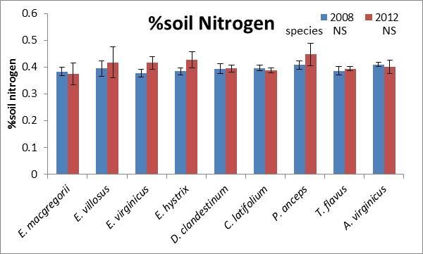
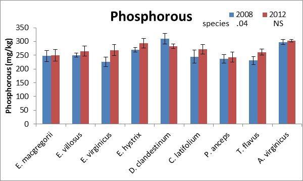
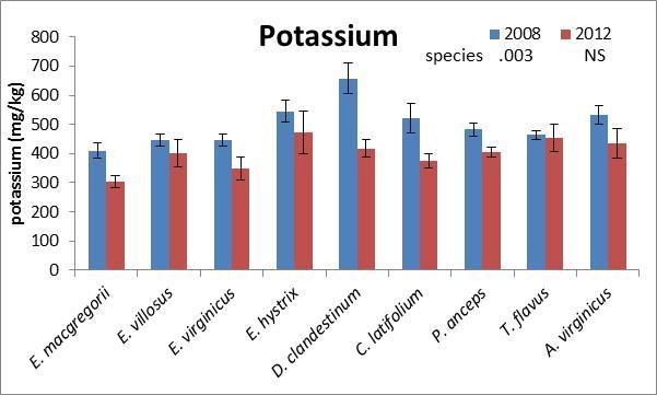
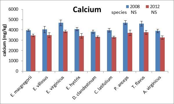
95 106

96 Figure 3.9: Left side panel shows averages (+/- 1 stderr) for soil nutrients (mg/kg), ph and buffer ph for 2008 and P values for species differences for 2008 and 2012 are denoted underneath the legend. Different letters represent significant differences between mean (P value 0.05). The right side panel shows averages (+/- 1 stderr) for the differences between 2012 and 2008 for soil nutrients, ph and buffer ph. Only soil ph had a significant species effect. 107

97 Chapter 4: Grazing strategies of C 3 and C 4 bunchgrasses native to a historic Oak Savanna-Woodland Abstract Since oak savannas of North America have been reduced to < 1 % of their historic ranges, restoration of these habitats is important to maintain the biodiversity and ecosystem properties of these landscapes. Restoration efforts of oak savannas are hindered by the lack of dependable historic data describing these savannas before they were converted to other uses and by lack of guidelines for ecological restoration. To better understand the dynamics associated with grazing effects, nine native bunchgrasses were studied in a clipping experiment that was designed to assess the effects of grazing on a savanna-woodland where no remnants remain to be studied, to compare the species for evidence of differences in grazing strategy (tolerance, deterrence and avoidance) and to recommend effective mowing regimes that would maintain a functional grassland community setting of the historic Bluegrass Oak Savanna-Woodland of Kentucky. This clipping experiment included a factorial design with two clipping frequency treatments and two clipping intensity treatments to mimic a range of grazing regimes from frequent intense grazing to less intense rotational grazing. A non-clipped control treatment was added for comparison. In a heated greenhouse, the clipping treatments lasted from June to September of 2010 with 14 weekly clippings and 4 monthly clippings at both a 7 and 15 cm height (intensity). Plant height, tiller number, and clipped wt. were recorded at each clipping. Root wt. and shoot wt. were harvested at the end of the experiment. Percent tissue C and % tissue N were assessed for the root wt. and shoot wt. This experiment included three C 4 and six C 3 native perennial bunchgrasses. Four of the C 3 grasses were from the genus Elymus which were well recorded in historical documents and have significant life history trait differences compared to the other six species. I found a significant effect of clipping on grass productivity overall, and a significant intensity effect but no significant frequency effect overall, and for the microscopic traits (tissue C/N) considered separately. For the macroscopic traits (productivity, biomass) considered separately, a significant frequency effect was detected but only at the most intense clipping treatment. In general, the three C 4 species and Dichanthelium clandestinum outperformed the Elymus species and Chasmanthium latifolium. All species except for Elymus macgregorii and Panicum anceps displayed evidence of more than one grazing strategy. While the most obvious strategies were seen at the 1/week 15 cm intensity clipping treatment, all nine species also were productive at the 1/month frequency treatments. Although grazing tolerance and deterrence strategies were mostly determined by clipping treatments, the avoidance strategy was more species specific with only D. clandestinum and Andropogon virginicus demonstrating an 108

98 avoidance strategy. D. clandestinum was the most plastic species, and the only one to demonstrate all three grazing strategies. The results of this experiment suggest that the Bluegrass Savanna-Woodland grassland was historically not frequently and intensively grazed. Mowing regime recommendations to sustain a community setting of these grasses would include less intense more frequent grazing, or more intense less frequent mowing treatments. The diversity of forbs and the control of woody vegetation also should be taken into account when determining a mowing regime, particularly when managing the Bluegrass Savanna-Woodland without the use of fire. Introduction Savannas are grassland ecosystems characterized by the trees being sufficiently small or widely spaced so that the tree canopy is not closed (McPherson 1997) and are influenced by fire, climate, topography and soil (Nuzzo 1986). Savannas cover 20 % of the Earth s land area and can be divided into tropical and temperate groups. Tropical savannas cover 15 % of the Earth s land area, are generally well represented in the scientific literature, and are extensive in Africa, Australia, and S. America (McPherson 1997). While temperate savannas of North America were historically common at the time of European settlement, most of these landscapes have been reduced to < 1 % of their original area, are considered to be endangered landscapes (Anderson, Fralish et al. 1999), and are identified as critical areas for preservation (Klopatek, Olson et al. 1979). Furthermore, temperate savannas are not as well studied or represented in the scientific literature (McPherson 1997, Anderson, Fralish et al. 1999). Some potential reasons for this difference in level of research activity are the absence of a professional discipline associated with savannas, limited understanding of the role and importance of savannas in temperate regions, and inconsistent definitions and/or interpretations of the term savanna (McPherson 1997). Thus, there is a lack of knowledge of the ecological relationships and ecological management practices for temperate savannas compared to adjacent forest, desert, or grassland landscapes (McPherson 1997). With European settlement in the eighteenth century, Midwestern Oak savannas in the U. S. A. all but disappeared within 20 to 40 years due to fire cessation and conversion of land to agricultural or urban development (Nuzzo 1986, Anderson, Fralish et al. 1999). The fact that only 2 % of Midwest Oak Savanna remained by 1986 (Nuzzo 1986) has caused this habitat to be listed as a globally imperiled ecosystem (Heikens and Robertson 1994). Conservation and restoration efforts of Oak Savannas are difficult due to: 1) the limited amount of historical data which were recorded, mainly by European pioneers and land surveyors, and the unknown validity and motivation for these records (Nuzzo 1986), and 2) lack of restoration ecology studies to guide ecological restoration practices in the field (McPherson 1997). 109

99 This restoration ecology study is designed to provide ecological guidelines to create and maintain a functional grassland community in the region where oak savanna once occurred. However no remnants remain to be studied and replicated, and the factors that created and maintained the savannas are unknown. A plant trait approach was used which views a species as a set of inter-connected traits that are both the result of its evolutionary history and the ability of the species to respond to or affect community biotic and abiotic factors (Adler, Milchunas et al. 2004). This plant trait approach can reveal what ecological pressures a species may have evolved under and also help predict how the species will adapt to future selective pressures. With this approach, past ecological pressures and historical disturbance regimes can be inferred by studying plant traits in response to different environmental factors. Disturbance is important and necessary for the maintenance of savannas. Frequent low intensity fires, a distinct annual dry season, extended droughts, and grazing by large herbivores are disturbances that often are associated with savannas (Enger and Smith 2004). However, these disturbances may be more characteristic of African Tropical Savannas than Midwestern Oak savannas (McPherson 1997). For example, the climate of most Midwestern Oak savannas does not promote frequent natural fires or extended droughts, and the dry season is generally more variable. While natural fires may not be common in Midwestern Oak savannas, fire is considered to be an important disturbance in the maintenance of Oak Savannas with Native Americans playing an important role (Mann 2011). The Bluegrass Savanna-Woodland located in the Inner Bluegrass Region of Kentucky was considered by Braun (1943) to be anomalous or unexpected in the middle of the mixed mesophytic forest biome. Wharton and Barbour (1991) characterized this area as a savanna-woodland with an open forest whereby the trees are dominant but with a well-developed grassy undergrowth. This savanna-woodland was best described at the time of European settlement in the mid to late 1700 s as having a mildly karst rolling topography, fertile, deep, and well drained silt loam soil produced over highly phosphatic Ordovician Limestone, vast cane breaks (Arundinaria gigantea), large mature trees including Oak (Quercus sp.) and Ash (Fraxinus), and a graminoid dominated herbaceous layer (McInteer 1952, Wharton and Barbour 1991, Campbell 2004). With European settlement, native grasses were rapidly replaced by non-native C 3 forage grasses (Poa pretensis and Festuca arundinacea) so that no intact savanna grassland remains in this region (Bryant, Wharton et al. 1980). It is thought that C 3 grasses were dominant in both abundance and number in the original savannas (Wharton and Barbour 1991, Campbell 2004), and that C 4 grasses fewer in the number of species and occurred in local openings on poorer soils or openings created by disturbance such as fire or bison trails (Campbell 2004). 110

100 Using Nuzzo s classification (1986), the Bluegrass savanna-woodland would have been classified as an open savanna that was maintained by frequent low intensity fires set by Native Americans (Mann 2011). Good evidence that the barrens in the Mississippian Plateau Region just west of the Bluegrass Region of Kentucky were created and maintained by anthropogenic fire (Anderson, Fralish et al. 1999) is further evidence that fire was used in this area. The use of fire by Native Americans may have been used in part to manage the large grazers or browsers of this system which were bison (Bison bison), elk (Cervus canadensis), and white tailed deer (Odocoileus virginianus) at the time of European settlement (Wharton and Barbour 1991). If these savanna grasslands evolved under heavy grazing, native grasses would be expected to have been selected for strategies to tolerate, avoid, or deter grazing. Furthermore, the grazing history of this Bluegrass Savanna-Woodland can be inferred by studying the response of native grasses to differing grazing intensities and frequencies. Augustine and McNaughton s (1988) review of clipping experiments found that the frequency of clipping had a bigger impact than the intensity of clipping. After grasses are grazed, the timing between grazing events was important because competition for the newly available light is time sensitive (Augustine and McNaughton 1998). The three grazing strategies optimize different suites of traits. Tolerance grazing strategies include rapid regrowth of tillers using the newly available light that was created by the grazing event, thus the grazing tolerant plant can outcompete its neighbors for light (Augustine and McNaughton 1998). Plant traits associated with grazing tolerance are increased photosynthetic rate, regrowth of photosynthetic biomass, lower investment of reproductive shoots, increased relative growth rates, increased root/shoot ratio, decreased C:N ratios, plasticity in carbon and nitrogen allocation, and reduced transpiration costs (Caldwell, Richards et al. 1981, Vandermeijden, Wijn et al. 1988, Augustine and McNaughton 1998, Pontes, Soussana et al. 2007). Grazing tolerant strategies are optimal under high grazing intensity and frequency environments where shading by neighboring plants is not an important factor. Strategies to deter grazing include the production of toxic secondary compounds or with mutualistic relationships with endophytes, and the accumulation of silica and/or recalcitrant carbon (Augustine and McNaughton 1998, Melo 2010). Grazing deterrence strategies promote the unpalatability of grasses that lower digestibility and nutritional value for herbivores. The avoidance grazing strategy is to be less conspicuous to herbivores and includes a low growth stature with low apical meristems, increased allocation to crown and roots, increased root/shoot ratio, and accumulation of standing senesced leaves and stems (Milchunas and Noy-Meir 2002, Adler, Milchunas et al. 2004, Quiroga, Golluscio et al. 2010). Structural carbon also would be important for the accumulation of aboveground dead biomass. Both avoidance and deterrence strategies are dependent on herbivore selection and preference, so these 111

101 strategies would be most beneficial in environments of intermediate grazing intensity and frequency where a variety of plants would be available for the herbivores (Vesk and Westoby 2001). A greenhouse clipping experiment was designed using six C 3 and three C 4 native bunchgrasses (Wharton and Barbour 1991, Campbell 2004) to assess tolerance and look for evidence of other grazing strategies of these nine grasses and infer the historic grazing pattern for each of them. A factorial design included two clipping heights (intensities) and two clipping frequencies that were designed to mimic a range of grazing regimes from intensive grazing to rotational grazing. A control treatment was added for comparison. I hypothesis that: 1) frequency will have a bigger impact on plant traits than intensity as predicted by Augustine and McNaughton (1998), 2) the C 4 species will be better adapted to grazing than the C 3 grasses because they generally have higher nitrogen use efficiency, a higher C:N ratio, and a higher water use efficiency that should make them less affected by biomass loss, 3) that the grasses may have different grazing strategies at different frequency and intensity treatment levels. Results of this experiment can be used to recommend mowing regimes for ecological restoration that will maintain these grasses in a community setting, and provide insights for future restoration efforts. Methods Experimental Design This clipping experiment was conducted using nine perennial bunchgrasses (six C 3 and three C 4 ) (Table 4.1) in a heated greenhouse at the University of Kentucky. A factorial design was used that included two clipping frequencies (1/week and 1/month) and two clipping heights (hereafter intensities; clip down to 7 cm and 15 cm above the soil surface) with a non-clipped control added for comparison. With a replication of 5, this completely randomized experiment produced 225 experimental units. An experimental unit consisted of one plant grown in a 16.6 cm depth, 16 cm width pot with drainage holes filled with 50% maury silt loam treated with methyl bromide, 50% coarse silica sand, and 15 milliliters of osmocote fertilizer. Seeds of each species were collected in the Bluegrass Region of Kentucky and cold (moist) stratification requirements were determined by the seed testing laboratory at the Regulatory Services at the University of Kentucky. Plants were stratified as needed, and placed to germinate on a flooding table in a heated greenhouse on January 28, They were grown in the 72-well plant trays filled with Pro- Mix potting mix soil before being transferred into the experimental pots on April 6, 2010 when they were completely randomized on greenhouse tables. The plants were hand watered with a hose as needed, and maximum and minimum temperatures of the greenhouse were recorded weekly (Figure 4.1). The grasses were grown in the experimental pots for 10 weeks before the clipping treatments began. 112

102 Clipping treatments began on June 15 th and lasted for 14 weeks until September 14 th. Before each clipping, maximum plant height, number of tillers, and number flowering culms were recorded. To clip down to 7 cm or 15 cm, a metal collar that was either 7 cm or 15 cm tall was put around the plant and rested on the soil surface. The plant biomass above the collar was then clipped, dried at 55º C for 3 days, and weighed. Fourteen weekly and 4 monthly plant measurements were recorded. The 1week 7 cm treatment was designed to mimic intense grazing. The 1 week 15 cm treatment represented less intense grazing, and the 1 month 7 cm treatment simulated intense rotational grazing and the 1 month 15 cm treatment simulated less intense rotational grazing. The control treatment mimicked no grazing. At the end of the experiment, shoots and roots were harvested, dried, and weighed. The roots were thoroughly rinsed over a mesh screen to remove as much sand and soil as possible. After the roots and shoots were dried and weighed, they were ground in a coffee grinder and analyzed for total %carbon and total %nitrogen with the Elementar vario MAX CNS Analyzer at the soils laboratory at Regulatory Services at the University of Kentucky. Species The nine native bunchgrasses (Wharton and Barbour 1991, Campbell 2004) included in this study are listed in Table 4.1 in the order of their flowering times. The nine species are categorized in two functional groups C 3 (or cool season) grasses and C 4 (or warm season) grasses. According to Wharton and Barbour (1991), the six C 3 grasses included in this study are associated with wooded habitats, and the three C 4 species are associated with more open habitats. Of the C 3 grasses, four species are from the genus Elymus or wildryes. Elymus species are well documented in historical records and are thought to have been abundant at the time of European settlement in the mid to late 1700 s (Wharton and Barbour 1991). E. virginicus is common in open woods, thickets and old fields, and E. villosus is frequent in dry and moist open woods (Wharton and Barbour 1991). E. macgregorii can be confused with E. virginicus but flowers a month earlier and is also found in woods and thickets (Committee 2002), and E. hystrix is frequent in woods (Wharton and Barbour 1991). The Elymus species have a different life history pattern with significant niche differentiation from the other five species used in this study. They flower in the spring or early summer, set seed, and then go dormant during the hottest months of the summer. Plants regrow tillers in the autumn that will overwinter and produce flowering culms the next spring. Dichantheilium clandestinum, which may have been referred to as buffalos grass in historical records, is frequent in open woods, thickets, and fencerows, especially on low ground (Wharton and Barbour 1991). D. clandestinum also has life history traits that differ from the other species in this study. D. clandestinum first produces cleistogamous flowering culms in the spring, and then later in the season plants produce self-fertilizing chasmogamous flowers on small inflorescences that are usually hidden 113

103 within the sheathes. Both types of flowers produce viable seeds. While this species did not produce a lot of tillers, it had the greatest ability for tiller branching, so one tiller could be quite large and heavy. C. latifolium is frequent on wooded stream banks, on floodplains, and in other moist habitats (Wharton and Barbour 1991), and it is used for in horticultural plantings and can be quite invasive. The three C 4 species used in this study generally are found in more open sites. P. anceps is found less commonly and on moist ground, and T. flavus is common in old fields, woodland borders, open woods, pastures, and roadsides (Wharton and Barbour 1991). A. virginicus is common in old fields and overgrazed pastures (Wharton and Barbour 1991). Plant traits Macroscopic and microscopic traits were recorded for each species. The macroscopic traits are morphological and were counted by observation (tiller number and number of flowering culms), measured (plant height), or weighed (shoot wt. root. wt., and clipped wt.). Tiller size was calculated by dividing the shoot wt. by the number of tillers (grams/tiller). Aboveground Net Primary Production (ANPP) represents the shoot wt. plus the clipped wt. For the control treatment, the shoot wt. was also used for ANPP as no clipping occurred. Total plant biomass is the sum of ANPP and the root wt. The microscopic traits are physiological in nature and include measurements of % total N or % total C and were not directly measured or observed. Percent C and % N in both roots and shoots were analyzed with the Elementar vario MAX CNS Analyzer. Shoot C and Shoot N represent the total amount of C and N in the shoot and were calculated by multiplying the biomass of the shoot by the % C or % N of the shoot. Root C and root N were calculated in the same way. % C:N shoots, % C:N roots, shoot C:N and root C:N are the ratios of the respective numbers. Considering the plant traits that were measured in this experiment, the three grazing strategies would optimize different suites of traits. Grazing tolerant plants would optimize regrowth (% N shoot, clipping wt.), which would lower shoot C:N and minimize sexual reproduction (number of flowering culms). The traits that would be optimized are clipped wt., percent shoot N, and root:shoot ratio, and minimize the number of flowering culms. Grazing deterrence strategies would optimize root:shoot ratio, % C shoot, shoot C, and C:N ratio, and minimize plant height, and the amount of N in the shoot. A tolerant plant would try to regrow tillers with the new light availability that was created by the grazing event, which would increase % N shoot, clipping wt. and plant height (Table 5). Statistics The statistical program PAST (Hammer 2001) was used to normalize the data and each ANOVA was performed in SAS (9.3: SAS Institute, Cary, NorthCarolina, USA) using PROC GLM (SAS 2010). Adhoc Tukeys tests were used for pairwise comparisons. To incorporate the control treatment into the 114

104 factorial 2x2 design, a partially hierarchical design was used. This design included the following factors: species (9 levels), group (2 levels: control vs. all others), frequency (nested within group; 2 levels: monthly vs. weekly), intensity (nested within group; 2 levels: 7cm vs. 15cm), as well as all identifiable two-way and three-way interactions. The total number of treatment combinations was 45. This analysis approach allowed us to test for main and interaction effects for each trait. Type I Sums of Squares were used to test these effects. Multivariate analysis was performed in the program PC-ORD (6.08: MjM Software, Gleneden Beach, Oregon, U.S.A.) using Principle Components Analysis (PCA) using the Euclidean distance measurement (McCune and Mefford 2011). The data were not standardized and all response variables were included in the analysis. The Euclidean distance measurement also was used with Multi-Response Permutation Procedures (MRPP) within PC-ORD to discern significant differences between the nine species, five treatments (1wk7cm, 1wk15cm, 1mnth7cm, 1mnth15cm, and control), three intensities (7cm, 15cm, and control) and three frequencies (1week, 1month, and control). MRPP also was used for pairwise comparisons using the Euclidean distance measurement. For the MRPP analysis, acceptable p values were determined by dividing 0.05 by the number of treatments. For intensity and frequency effects, the acceptable p<0.017, for treatment effects p<0.01, and for species p< All pairwise comparisons used p<.025. Results Maximum weekly temperatures taken in the greenhouse were consistently and significantly higher than ambient maximum monthly temperature averages for Fayette County, Kentucky (Figure 4.1). Thus, the plants experienced higher than average maximum temperatures in the greenhouse than they would have experienced in the field. The high heat in the greenhouse during this experiment was probably most detrimental to the Elymus species because under field conditions, these species would have been dormant at that time. The number of plants that died during the experiment was higher in the 1/week frequency than the 1/month treatments with only Elymus species dying (Table 4.2). Also, one plant of E. villosus and A. virginicus died in the controls (Table 4.2). Group, Species and Treatment Effects:ANOVA Overall, there were significant effects of group (C 3 vs. C 4 ), species, intensity and frequency on macroscopic traits (Table 4.4) as well as numerous interactions. In multiple comparison, with the exception of total clipped weight (Figure 4.5), the three C 4 species and D. clandestinum produced significantly more total plant biomass, ANPP, and number of flowering culms than the four Elymus species and C. latifolium (Figure 4.5). T. flavus produced more shoot wt. than the four Elymus species and C. latifolium (Figure 4.5). P. anceps, T. flavus, and D.clandestinum produced more root wt. and grew 115

105 fewer but bigger tillers than the other species (Figure 4.5). T. flavus, and P. anceps increased plant height significantly more than the four Elymus species and D. clandestinum. P. anceps and D. clandestinum had a significantly higher root:shoot compared to E. macgregorri and E. hystrix (Figure 4.5). For the microscopic traits (Table 4.5 and Figure 4.6), a significant species effect was detected for all traits except for % C roots. The same as the whole model species pattern (Figure 4.4 D), the C 4 species and D. clandestinum had significantly higher % C:N root and % N root than the four Elymus species and C. latifolium (Figure 4.6). The C 4 species and C. latifolium were significantly higher in % C:N shoots, % N shoots, and shoot C:N than the four Elymus species and D. clandestinum (Figure 4.6). There were no clear species grouping patterns for %C shoots, shoot C, shoot N, root C:N, root C, and root N (Figure 4.6). Group, Species and Treatment Effects:PCA To simplify the analysis and examine these overall results in more depth, PCA was used to organize the trait responses into more inclusive, correlated categories. In the multivariate PCA analysis using all plant traits, significant intensity, frequency, treatment, and species differences were found (all p<.0001) (Figure 4.2A-D). The axes aggregate the traits fairly cleanly into macroscopic (Axis 1) and microscopic (Axis 2) traits. Many of the significant differences were primarily on Axis 1, but Axis 2 played a role as well. While intensity showed significant differences between all three treatments (7cm, 15 cm and control) (all p<.0001), the two frequency treatments (1/week and 1/month) were significantly different from the control (p<.0001) but not significantly different from each other (p=.06) (Figure 4.2A and B). When the PCA analysis was grouped by treatment, all four factorial clipping treatments were significantly different from the control (Figure 4.2C). There was an intensity effect with the two 15 cm treatments being significantly different than the two 7 cm treatments but no frequency effect. When the PCA analysis was grouped by species, two species groupings were apparent with the four Elymus species and C. latifolium in one group, and the three C 4 species and D. clandestinum in the other group (Figure 4.2D). In multivariate space, overall, the three C 4 species and D. clandestinum were more productive, and the four Elymus species and C. latifolium were the least productive (Figure 4.2D). T. flavus was the most productive species. A separate PCA analysis was performed for the macroscopic and the microscopic traits to discern if these two types of traits were affected differently (Figure 4.2E and F). The macroscopic axes (Figure 4.2E) now separate out into productivity (Axis 1) and allocation (Axis 2), and the microscopic axes (Figure 4.2F) are less clear but appear to be root N (Axis 1) and shoot N (Axis 2). Both types of traits were significantly affected by intensity, frequency, treatment and species (all effects p<.0001) (Figure 4.2E and F). For the macroscopic traits, all three intensity treatments (7 cm, 15 cm and control) and all 116

106 three frequency treatments (1/week, 1/month and control) were significantly different (all effects p<.0001). Species Differences at each Treatment Level A PCA analysis was performed for each of the five treatments and grouped by species (Figure 4.4) to compare how the species were grouped at each treatment level compared to the overall model pattern using all treatments (Figure 4.2D). The same general species grouping between the four Elymus species plus C. latifolium, and the three C 4 species plus D. clandestinum (Figure 4.2 D) was found for both of the 15 cm intensity treatments (1week15cm and 1month15cm) (Figure 4.4 B, and D). The 1month7cm treatment (Figure 4.4 C) was similar to the overall pattern using all treatments (Figure 4.2 D) except T. flavus was significantly more productive than the other species. For the control treatment, all the species are loosely grouped but T. flavus was significantly more productive than the other species (Figure 4.4 E). For the 1week 7cm treatment, there is no clear grouping of species except that E. macgregorri did significantly worse than all the other species (Figure 4.4 A). Pairwise comparisons were done using MRPP for all treatment combinations, which are shown in Table 4.3. The shaded cells represent a significant difference between the two treatments at that frequency or intensity level. If a frequency cell is shaded, the interpretation is that there is a significant intensity effect between those two frequency treatments. If an intensity cell is shaded, the interpretation is that there is a significant frequency effect between those two intensity treatments. When pairwise comparisons were done at the treatment level for the macroscopic traits, a significant frequency effect was found between the two 7 cm intensity treatments (Table 4.3). This significant frequency effect between the two 7 cm intensity treatments was not detected in the overall model (Table 4.3). Similar to the overall model, significant intensity effects were found when comparing both frequency treatments at both 1/week and 1/month intensity treatments. When the analysis was grouped by species, the species groupings also were different looking at just the macroscopic traits compared to the overall pattern using all plant traits (Figure 4.2 D and E) with the four Elymus species being loosely grouped and all other species being significantly different from each other. For the four Elymus species, E. villosus was statistically the same as E. macgregorri and E. hystrix, and E. virginicus was statistically the same as E. hystrix. (Figure 4.2E). For the microscopic traits, intensity and frequency had the same effects as the whole model using all plant traits. Intensity was significantly different between all three treatments (7 cm, 15 cm and control), and the two frequency treatments (1/week and 1/month) were significantly different from the control (both p<.0001) but not significantly different from each other (p=.06). When pairwise comparisons were done at the treatment level, significant intensity effects were found between the two levels at the 1/week frequency and between the two levels at the 1/month frequency (Table 4.3). This was the same pattern as the overall model using all plant traits. Species groupings for the microscopic traits were similar to the 117

107 overall pattern using all plant traits (Figure 4.2 D and F). The only difference was that A.virginicus (Broom) and P. anceps were not significantly different in the microscopic plant trait analysis (Figure 4.2 D and F). Treatment Differences for each Species Another PCA analysis was performed for each species and grouped by treatment using all plant traits (Figure 4.7). E. macgregorri, E. villosus, and E. hystrix were the only species to have treatments that were not significantly different from the controls (Figure 4.7). Looking at the PCA analysis done for each species that included all plant traits (Figure 4.7), all nine species had a significant intensity effect (all species p<.0007) but only E. virginicus and D. clandestinum had a significant frequency effect (both species p<.0001). For each species, pairwise comparisons were done using MRPP for all treatment combinations (Table 4.3). The shaded cells represent a significant difference between the two treatments at that frequency or intensity level. If a frequency cell is shaded, the interpretation is that there is a significant intensity effect between those two frequency treatments. If an intensity cell is shaded, the interpretation is that there is a significant frequency effect between those two intensity treatments. No clear patterns were seen between C 3 and C 4 species. Looking at all plant traits, all nine species had a significant intensity effect between the two 1/week frequency treatments, and six species had a significant intensity effect between the two 1/month frequency treatments (Table 4.3). Five species had significant frequency effects at both intensity levels (Table 4.3). Comparing the macroscopic and microscopic traits, the macroscopic traits had more species with significant frequency effects at both levels of intensity, and the microscopic traits had more species with intensity effects at both levels of frequency (Table 4.3). For the microscopic traits, all nine species had significant intensity effects at both frequency levels (Table 4.3) with five species had significant frequency effects at the 7 cm intensity level and three species had frequency effects at the 15 cm intensity level (Table 4.3). For the macroscopic traits, seven species had a significant intensity effect between the two 1/week frequency treatments, and seven species had a significant frequency effect between the 7 cm intensity treatments (Table 4.3). Four species had significant intensity effects at the 1/month frequency and four species had significant frequency effects between the 15 cm intensity treatments. E. macgregorii was the only species with the same effects for all plant traits, macroscopic traits, and microscopic traits (Table 3). P. anceps was the only other species besides E. macgregorri to have the same macroscopic and microscopic effects. Four C 3 species (E. villosus, E. hystrix, D. clandestinum, and C. latifoium) had the same effects for all plant traits and microscopic traits (Table 4.3). T. flavus and E. virginicus had different effects for all plant traits, macroscopic traits, and microscopic traits (Table 4.3). 118

108 Grazing strategies Since a species was predicted to show different grazing strategies at different treatment levels, a PCA analysis was done using all plant traits for each species and grouped by the five treatments (Figure 4.7). To discern how each species responded to the clipping treatments, another PCA analysis was performed for each species with the control excluded (Figure 4.7). With the plant traits measured in this experiment, I categorized the most important plant traits for each grazing strategy and designated if the trait was positively or negatively correlated with that grazing strategy (Table 4.6). For each species, I assessed the grazing strategy at each clipping treatment level by determining what traits were positively or negatively correlated on the PCA graph according to each strategy (Table 4.7). Those predictions were verified using Figures 3.5, 3.6 and Supplemental graphs. If a treatment did not have a discernable pattern, it was left blank (Table 4.7). While these results are somewhat subjective, I found evidence of all three grazing strategies. A treatment received a tolerance designation if it had an increased level of % N shoot along with increased clipped wt. and/or plant ht. (Figures 3.5, 3.6, and 3.7). Evidence of the tolerance strategy was found only at the 1/week frequency level treatments and for every species except for A. virginicus (Broom) and D. clandestimum (Table 4.7). In general, the Elymus species did not grow well at the 1/week 7cm treatment level and could not sustain the tolerance strategy throughout the experiment (Figure 4.5 and Supplemental). At the 1/week 15cm treatment, E. macgregorii, E. virginicus and E. hystrix were able to maintain the tolerance strategy but they did not maintain as much clipped wt. as C. latifolium (Supplemental). At the 1/week 7cm treatment level, D. clandestinum had higher clipped wt. than C. latifolium and T. flavus (Figure 4.5 and Supplemental). E. villosus, P. anceps, and T. flavus were designated as tolerant at the 1/week 15 cm treatment because %N shoot was positively correlated to plant ht. (Figures 3.5 and 3.6). P. anceps at the 1/week 7 cm treatment also was designated at tolerant. At the 1/week 15 cm treatment, T. flavus produced more total plant biomass compared to the other three clipping treatments by investing more in shoot wt. and root wt. T.flavus also had the highest plant ht., shoot carbon, shoot nitrogen, root carbon and root nitrogen at 1/week 15 cm treatment compared to the other three clipping treatments (Figures 3.5 and 3.6). P. anceps responded similarly as T. flavus at the 1/week 15 cm treatment but also produced significantly more flowering culms at this treatment level (Figure 4.5). To assess the deterrence strategy, I predicted % C:N shoot, shoot C:N (high % C and low % N in shoots), and bigger tillers would be increased, while tiller number would be minimized (Table 4.6). The three C 4 species and C. latifolium had significantly higher % C:N shoots and shoot C:N and significantly lower %N shoots which implies they are better able to deter grazing than the other species (Figure 4.6). At the 1/month 7 cm clipping treatment, E. virginicus, E. hystrix, D. clandestinum, C. latifolium, T. flavus, and A. virginicus had the highest % C:N shoots compared to all five treatments (Figure 4.6). 119

109 These same six species plus E. villosus also had the lowest % N shoots at the1/month 7 cm clipping treatment (Figure 4.6). To assess the avoidance grazing strategy, I predicted that shoot wt., root wt. root:shoot, tiller number, root C, and root N would increase, while clipped wt., plant height, and tiller size would decrease (Table 4.6). The clearest evidence of the avoidance grazing strategy was found for D. clandestinum at the 1/week 15 cm treatment (Table 4.7). D. clandestinum allocated biomass to leaves and stems below the 15 cm clipping height, produce little clipped wt. while still producing as much biomass as the control (Figure 4.5). At the 1/week 15 cm treatment, D. clandestinum grew more tillers than the other three treatments (Supplemental) and invested more biomass in root wt. which gave it a high root:shoot ratio (Figure 4.5). D. clandestinum also had significantly more root C and N at the 1/week 15cm treatment than the other 4 treatments (Figure 4.6). The only other species that displayed avoidance traits was A. virginicus (Broom) which allocated more biomass and nitrogen to the roots, produced more tillers, and grew shorter plants at the 15 cm intensity treatments compared to the control treatment (Figures 3.5 and 3.6 and Supplemental). A. virginicus (Broom) was also characterized as avoidance at the 1/week 7 cm treatment because it responded similarly as at the 15 cm frequency treatment except for producing less root wt, and reducing clipped wt. instead of plant ht. (Figure 4.6). Discussion The intensity of clipping had a bigger effect than the frequency of clipping on the macroscopic and microscopic traits for all species except for E. virginicus and D. clandestinum (Table 4.3). For the overall multivariate analysis including all nine species and all plant traits, a significant intensity effect was detected but not a significant frequency effect with both levels of frequency with both levels of intensity being significantly different from the control (Figure 4.2 A and B). These results are opposite of what Augustine and McNaughton (1988) found in their review of clipping experiments. My results may not support the conclusions of Augustine and McNaughton (1998) because 1) the short length of time the experiment was conducted, and 2) temperate bunchgrasses may not be as grazing tolerant as the tropical species they generally used in their review. When a separate PCA analysis was performed on the macroscopic and microscopic traits, a significant frequency effect was detected for the macroscopic traits between the two 7 cm intensity treatments (Table 4.3). Thus, frequency became important when the grasses were more intensively clipped. The species were more significantly different between the macroscopic than the microscopic traits (Figure 4.3 E and F). A frequency effect at lowest intensity treatment was seen for E. macgregorii, E. virginicus, P. anceps and T. flavus for the macroscopic traits and E. macgregorii, P. anceps and T. flavus for the microscopic traits (Table 4.3). When frequency and intensity effects were analyzed at the species level, all species had a significant intensity effect but only E. virginicus, and D. clandestinum had a significant frequency effect. At the treatment level analysis (Table 120

110 4.3), E. macgregorii, E. hystrix, P. anceps, and T. flavus had significant frequency effects for both macroscopic and microscopic traits, C. latifoium and A. virginicus had significant frequency effects for only the macroscopic traits, and E. villosus had no frequency effects (Table 3). It could be that frequency has a bigger effect on tropical species because they are better adapted to more intense grazing. The bunchgrass species used in this experiment seem to be better adapted to more frequent but less intense grazing events, therefore, they are more sensitive to intensity. Considering how the nine species performed in this greenhouse environment with no imposed clipping (control), the C 4 species produced the most total biomass, followed by C. latifolium and D. clandestinum, with the four Elymus producing the least amount of biomass (Figure 4.4 E). While the C 4 species were positively correlated to all the macroscopic traits, the C 3 species were positively correlated to only a few microscopic traits (Figure 4.4 E). The high heat in the greenhouse (Figure 4.1) and the life history traits of the Elymus species may have been partly to blame for the poor performance of the Elymus. When clipping treatments were added to the analysis, the C 4 species and D. clandestinum performed better than the other five C 3 species (Figure 4.2 D). The C 4 species generally outperformed the Elymus species in all macroscopic traits except for root:shoot and tiller number ( Figure 4.3B and Figure 4.5). Three of the Elymus species (E. macgregorri, E. villosus, and E. hystrix) had 15 cm intensity treatments that were not significantly different than the controls (Figure 4.7). This may indicate that these three Elymus species were not significantly affected at those treatment levels. C. latifolium performed similarly to the Elymus species in all macroscopic trait except that C. latifolium grew less tillers. D. clandestinum performed similarly to the C 4 species except D. clandestinum grew shorter plants with less clipped wt. (Figure 4.5). For the microscopic traits, the C 4 species and C. latifolium had lower tissue nitrogen concentrations in the shoots which gave them a higher shoot C:N compared to the other five C 3 species (Figure 4.3C and Figure 4.6). The C 4 species and D. clandestinum had lower tissue N in the roots that resulted in a higher C:N in the root compared to the other five species. Thus, the C 4 species had a higher a C:N ratio in both the root and shoot compared to the Elymus species, and the Elymus species had higher percent tissue N in shoots and roots. Grazing strategies This experiment was primarily designed to assess grazing tolerance rather than grazing deterrence and avoidance. Grazing deterrence and avoidance are dependent on herbivore selection which was not included in this design. However, the results can be interpreted from this broader perspective. In response to clipping, T. flavus was generally the top performer in all clipping treatments with P. anceps performing well at the 15 cm treatments, and D. clandestinum performing well at the 1 week 7 cm treatment (Figure 4.4). While the Elymus species and C. latifolium were the poorest performers at all treatment levels, E. 121

111 macgregorii performed the worst at the 7 cm intensity treatments (Figure 4.4). With higher percent shoot tissue N concentrations, the Elymus species and D. clandestimum would be expected to be able to replace eaten biomass and therefore be more grazing tolerant. With higher shoot C:N, the C 4 species and C. latifolium would generally be expected to be less nutritious and therefore deter grazing. While evidence for both of these strategies were found, these two grazing strategies were determined more by frequency and not by the C 3 and C 4 species grouping (Table 4.7). Only the avoidance strategy seemed to be species specific (Table 4.7). Evidence for tolerance strategies was found at the 1/week frequencies. The most clear example of tolerance was for T. flavus at the 1/week 15 cm treatment where increased concentrations of N was found in the root and shoot which was allocated to growing taller plants. Higher amount of N in the roots and shoots imply increased N uptake at the 1/week 15 cm treatment. An explanation for why the Elymus did so poorly at the 1/week 7cm treatments may be that plants could not sustain the tolerance strategy throughout the experiment. With the high % N demand of the shoots, N uptake from the soil may have become limited as the clipping continued until the plants died or looked necrotic. Since the Elymus species are generally found in more mesic low lands and shaded wooded areas, they may not be adapted for frequent high intensity clipping under high heat and light conditions. Evidence for the deterrence grazing strategy was found at the 1/month 7 cm treatment for all species except for E. macgregorii and P. anceps. Since the C 4 species and C. latifolium had higher C:N ratios than the C 3 species, they are expected to be better at deterring grazing. While this pattern was true for all of those species except for P. anceps, three of the Elymus species and D. clandestinum also had increased shoot C:N at the 1/month 7 cm treatment. Since species that are found in more open areas (C 4 species) and wooded areas (C 3 species) displayed deterrence strategies at the 1/month 7 cm treatment, there must be enough time between clippings at this lowest clipping intensity for plants to reallocate C to the shoots. D. clandestinum and A. virginicus (Broom) were the only species that exhibited traits that promoted the avoidance strategy (Table 6). D. clandestinum exhibited clear avoidance traits at the 1/week 15 cm treatment where it concentrated biomass below the clipping height and in the roots with reduced clipping wt. (Figure 4.5). D. clandestinum also was the most plastic species, since it responded significantly different between all treatments (Figure 4.7). A. virginicus (Broom) displayed avoidance traits at the 15 cm intensity treatments and the 1/week 7 cm treatment by allocating more biomass to roots, increasing % N root, increasing tiller number, and growing shorter plants (Figures 3.5 and 3.6 and Supplemental). A. virginicus (Broom) was also considered avoidance at the1/month 15cm treatments and 122

112 at the 1/week 7cm where it allocated more biomass and nitrogen to the roots, produced more tillers, and grew shorter plants (Figures 5 and 6). The avoidance strategy for A. virginicus may be optimal in habitats without intense light competition from other plants which may be why this species is found commonly in old fields and overgrazed pastures (Wharton and Barbour 1991). Conclusion In conclusion, my hypothesis that clipping frequency would have a bigger effect on these nine species than clipping intensity was not supported. I found clipping intensity to have a bigger effect for both macroscopic and microscopic traits than clipping frequency, and a clipping frequency effect was found for only the macroscopic traits at the most intense (7 cm) clipping treatment. I predict that these bunchgrasses should be more sensitive to intensity if these savanna-woodland grasses historically experienced frequent but less intense grazing. My second hypothesis was partially supported as the C 4 species were more productive than all the C 3 species except for D. clandestinum. D. clandestinum had the most plastic response to grazing, and it was the only species to display traits for all three grazing strategies. T. flavus was the most productive of the C 4 grasses, and the Elymus species, particularly E. macgregorri, were the least productive. The Elymus species were probably the least adapted to the high light and heat environment of the greenhouse which was at the same time they would have been dormant under field conditions. Dormancy of the Elymus species at the same time the other species are active also may be a good grazing avoidance strategy that was not assessed in this experiment. I also predicted that the Elymus species would be eliminated from this savanna-woodland grassland community under high frequency and intensity grazing regimes. My third hypothesis that these grasses would have different grazing strategies at different frequency and intensity treatment levels was supported for all the species except for E. macgregorii and P. anceps. The most obvious grazing strategies were at the 1/week 15 cm treatment where D. clandestinum displayed clear avoidance traits, T. flavus displayed clear tolerance traits, and P. anceps optimized sexual reproduction through the production of flowering culms. The results of this experiment suggest the Bluegrass Savanna-Woodland grassland was not historically intensively grazed at high frequencies but that these grasses may be able to sustain this level of grazing for a short time. These results also suggest that these grasses are more adapted to less intense more frequent grazing, or more intense less frequent grazing. Mowing regimes at these intensity and frequency levels would most likely maintain a community settimg of these grasses. However, since fire is thought to be an important tool to keep woody species at bay, when fire is not used as a management tool, woody species management also would have to be taken into account when prescribing mowing regimes to maintain the Bluegrass Woodland-Savanna landscape. In some savannas, light grazing has apparently helped to preserve the savanna by inhibiting woody invasion without eliminating the ground layer (Nuzzo 123

113 1986). To be able to manage higher diversity of the savanna-woodland, future clipping experiments should include other functional groups such as woody species and forbs. (Braun 1943) Literature Cited Adler, P. B., D. G. Milchunas, W. K. Lauenroth, O. E. Sala and I. C. Burke (2004). "Functional traits of graminoids in semi-arid steppes: a test of grazing histories." Journal of Applied Ecology 41(4): Anderson, R. C., J. S. Fralish and J. M. Baskin, Eds. (1999). Savannas, Barrens, and Rock Outcrop Plant Communities of North America. Cambridge, UK, Cambridge University Press. Augustine, D. J. and S. J. McNaughton (1998). "Ungulate effects on the functional species composition of plant communities: Herbivore selectivity and plant tolerance." Journal of Wildlife Management 62(4): Braun, E. L. (1943). Deciduous Forests pf Eastern North America. Philadelphia, Blakiston Co. Bryant, W. S., M. E. Wharton, W. H. Martin and J. B. Varner (1980). "The Blue Ash-Oak Savanna- Woodland, a Remnant of Presettlement Vegetation in the Inner Bluegrass of Kentucky." Castanea 45(3): Caldwell, M. M., J. H. Richards, D. A. Johnson, R. S. Nowak and R. S. Dzurec (1981). "COPING WITH HERBIVORY - PHOTOSYNTHETIC CAPACITY AND RESOURCE-ALLOCATION IN 2 SEMI-ARID AGROPYRON BUNCHGRASSES." Oecologia 50(1): Campbell, J. (2004). Comparitive Ecology of Warm-Season (C4) versus Cool-Season Grass (C3) Species in Kentucky, with Reference to Bluegrass Woodlands. 4th Eastern Native Grass Symposium University of Kentucky. Campbell, J. (2004). Comparitive Ecology of Warm-Season (C4) versus Cool-Season Grass Species in Kentucky, with Reference to Bluegrass Woodlands. 4th Eastern Native Grass Symposium University of Kentucky. Committee, F. o. N. A. E., Ed. (2002). Flora of North America: Magnoliophyta: Commelinidae (in part): Poaceae, part 1. New York, Oxford University Press. Enger, E. D. and B. F. Smith (2004). Environmental Science A Study of Interrelationships. Boston, McGraw Hill Higher Education. Hammer, Ø., Harper, D.A.T., Ryan, P.D. (2001). PAST: Paleontological statistics software package for education and data analysis. Palaeontologia Electronica P. Electronica. Heikens, A. L. and P. A. Robertson (1994). "Barrens of the Midwest: A review of the literature.." Castanea 59: Klopatek, J. M., R. J. Olson, C. J. Emerson and J. L. Jones (1979). "Land -use confict with natural vegetation in the United States.." Environmental Conservation 6: Mann, C. C. (2011) Uncovering the New World Columbus Created. New York, Vintage Books. 124

114 McCune, B. and M. J. Mefford (2011). PC-ORD. Multivariate Analysis of Ecological Data. Gleneden Beach, Oregon, U.S.A., MjMSoftware. McInteer, B. B. (1952). "Original Vegetation in the Bluegrass Region of Kentucky." Castanea 17: McPherson, G. R. (1997). Ecology and Management of North American Savannas. Tucson, Arizona, The University of Arizona Press. Melo, S. P., Francisco A. Monteiro, Fabioa Daniel De Bona (2010). "Silicon distribution and accumulation in shoot tissue of a tropical forage grass Brachiaraia brizantha." Plant Soil 336: Milchunas, D. G. and I. Noy-Meir (2002). "Grazing refuges, external avoidance of herbivory and plant diversity." Oikos 99(1): Nuzzo, V. A. (1986). "Extent and Status of Midwest Oak Savanna: Presettlement and 1985." Natural Areas Journal 6: Pontes, L. D. S., J. F. Soussana, F. Louault, D. Andueza and P. Carrere (2007). "Leaf traits affect the above-ground productivity and quality of pasture grasses." Functional Ecology 21(5): Quiroga, R. E., R. A. Golluscio, L. J. Blanco and R. J. Fernandez (2010). "Aridity and grazing as convergent selective forces: an experiment with an Arid Chaco bunchgrass." Ecological Applications 20(7): SAS (2010). SAS for Windows. S. Institute. Cary, NC, U.S.A. Vandermeijden, E., M. Wijn and H. J. Verkaar (1988). "DEFENSE AND REGROWTH, ALTERNATIVE PLANT STRATEGIES IN THE STRUGGLE AGAINST HERBIVORES." Oikos 51(3): Vesk, P. A. and M. Westoby (2001). "Predicting plant species' responses to grazing." Journal of Applied Ecology 38(5): Wharton, M. E. and R. W. Barbour (1991). Bluegrass Land and Life. Lexington, University Press of Kentucky. 125

115 Tables Table3.1: The nine native perennial bunchgrass species used in this experiment listed in order of flowering time. The abbreviations are used in the multivariate graphs. Scientific Name Abbrev Photosynthetic Common Name iation Pathway 1. Elymus macgregorii R. Brooks & J.J.N. Campb. Emg Early wildrye 2. Elymus villosus Muhl. ex Willd. Evl Nodding wildrye 3. Elymus virginicus L. Evg Virginia wildrye 4. Elymus hystrix L. Ehy Bottlebrush C 3 5. Dichanthelium clandestinum (L.) Gould Dclan Deer tongue 6. Chasmanthium latifolium (Michx.) Yates Clat River Oats 7. Panicum anceps Michx. Panc Beaked panicgrass 8. Tridens flavus (L.) Hitchc. Tflav Purple top/grease grass C 4 9. Andropogon virginicus L, Broom Broomsedge Table 4.2. Number of plant deaths for each species by treatment. Species Number of dead plants by treatment 1week7cm 1week15cm 1month7cm 1month15cm control Emg 1 Evl 2 1 Evg 1 Ehy 2 Dclan Clat Panc Tflav Broom 1 126

116 Table 4.3: PCA results for treatment effects for all plant traits combined, macroscopic traits, and microscopic traits. The P value is for the overall model for all species and each species. The shaded cells represent a significant difference (p<.025) between the two treatments at that frequency or intensity level. If an intensity cell is shaded, the interpretation is that there is a significant intensity effect between those two frequency treatments. If a frequency cell is shaded, the interpretation is that there is a significant frequency effect between those two intensity treatments. PCA results for significant treatment effects All species Emg Evl Evg Ehy Dclan Clat Panc Tflav Broom All plant traits P value < <.0001 <.0001 <.0001 <.0001 <.0001 <.0001 <.0001 Intensity (p<.025) 1/week 1/month Frequency (p<.025) 7cm 15cm Macroscopic traits Pvalue <.0001 < <.0001 <.0001 <.0001 <.0001 <.0001 <.0001 <.0001 Intensity (p<.025) 1/week 1/month Frequency (p<.025) 7cm 15cm Microscopic traits Pvlaue < <.0001 <.0001 <.0001 <.0001 <.0001 <.0001 <.0001 Intensity (p<.025) 1/week 1/month Frequency (p<.025) 7cm 15cm 127

117 Table 4.4 Whole model macroscopic traits ANOVA results including nine species, two clipping frequencies (weekly and monthly), 2 clipping intensities (7 cm and 15 cm), plus all interactions. Type I Sums of Squares were used to test these effects. Total biomass (grams) ANPP (grams) Shoot wt grams Root wt. (grams) Root:shoot Df F p F p F p F p F p Group < < < < <.0001 Species < < < < <.0001 Frequency < < Intensity < < < < <.0001 Freq*inten Spec*freq < < < <.0001 Spec*inten Sp*fre*int Plant ht Tiller size Tiller number (cm) (tiller#/grams) Df F p F p F p Group < <.0001 Species < < <.0001 Frequency < Intensity < < <.0001 Freq*inten < Spec*freq < <.0001 Spec*inten < < <.0001 Sp*fre*int <

118 Table 4.5 Whole model microscopic traits ANOVA results including nine species, two clipping frequencies (weekly and monthly), 2 clipping intensities (7 cm and 15 cm), plus all interactions. Type I Sums of Squares were used to test these effects. %C/%N shoot C/N shoot C shoot %C shoot %N shoot (grams/grams) (grams) Df F p F p F p F p F p Group < <.0001 Species < < < < <.0001 Frequency < < < <.0001 Intensity < <.0001 Freq*inten < < < Spec*freq < <.0001 Spec*inten Sp*fre*int N shoot (grams) %C root %N root C/N root %C:%N root (grams/grams)) Df F p F p F p F p F p Group < < < Species < < < <.0001 Frequency < Intensity < Freq*inten < Spec*freq < < Spec*inten Sp*fre*int

119 C root N root (grams) (grams) Df F p F p Group Species < <.0001 Frequency Intensity < <.0001 Freq*inten Spec*freq < <.0001 Spec*inten Sp*fre*int Table 4.6: Plant traits that are predicted to signify the three different grazing strategies that are denoted with a ( ) if positively correlated and ( ) if negatively correlated. Grazing strategies Tolerance Deterrence Avoidance Macroscopic traits Total plant biomass ANPP Shoot wt. Total clipped wt. Root wt. Root:shoot Cumulative plant height Tiller number Tiller size Flowering culms Microscopic traits %C/N shoots %C shoots %N shoots Shoot C/N Shoot C Shoot N %C/N roots %C roots %N roots Root C/N Root C Root N 104

120 Table 4.7: Assessment of observed grazing strategy patterns for each species at each clipping treatment. The grazing strategy designations were determined by comparing the expected trait correlations for each strategy in Table 4.6 and comparing these predictions to Figures 3.5, 3.6, 3.7 and Supplemental. Grazing strategy predictions Species 1/week 7 cm 1/week 15cm 1/month 7cm 1/month 15cm Emg tolerance tolerance Evl tolerance tolerance deterrence Evg tolerance tolerance deterrence Ehy tolerance tolerance deterrence Dclan tolerance avoidance deterrence Clat tolerance tolerance deterrence Panc tolerance tolerance Tflav tolerance tolerance deterrence Broom avoidance avoidance deterrence avoidance 105

121 Figures Figure 4.1: Maximum and minimum greenhouse temperatures (ºC) recorded from the time the seeds germinated until the end of the 3 month clipping experiment. Max and min monthly averages for Fayette County in 2010 were added for comparison (Ky Mesonet). 106

122 Whole model by intensity A. B ShootN control %Nshoot Axis 2 (15.3%) ShootC tillsize 15cm shtwt rootc rootn totbio rootwt ANPP culms plntht RootCN %CNroot ShootCN %CNshot clipwt Axis 1 (42.6%) 7cm %Crooot %Nroot C D E. F Figure 4.2: PCA results A.) all traits grouped by intensity, B.) all traits grouped by frequency, C.) all traits grouped by the five treatments, D.) all traits grouped by species. E.) macroscopic traits grouped by species, and F.) microscopic traits grouped by species. The circles represent the species means that are not significantly different in pairwise comparisons using MRPP (p<.025). The percent of variance explained for each axis is in parenthesis. 107

123 A. B. C. Figure 4.3: PCA results for the clipping treatments only A.) all traits with the control treatment excluded, B.) macroscopic traits with the control treatment excluded, C.) microscopic traits with the control treatment excluded. The circles represent the means that are not significantly different in pairwise comparisons using MRPP (p<.025). The percent of variance explained for each axis is in parenthesis. 108

124 A B C D E. Figure 4.4. PCA results for each treatment using all traits grouped by species. The circles represent the species means that are not significantly different in pairwise comparisons using MRPP (p<.025). The percent of variance explained for each axis is reported. 109

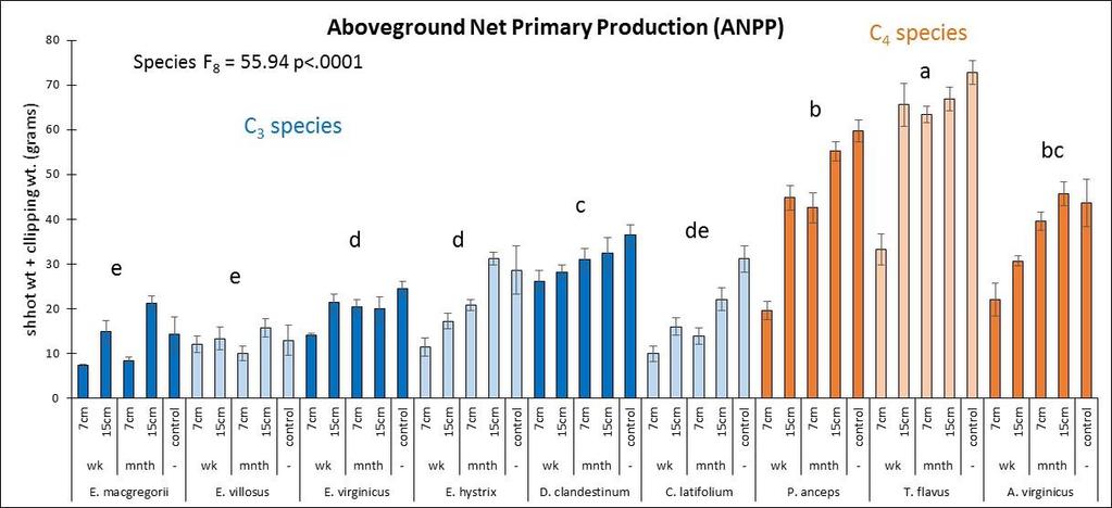
125 110

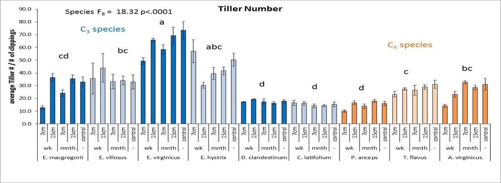
126 111

127 Figure 4.5: Macroscopic variables with treatment means (±SE) for each species. The species are listed on the x-axis in order of their flowering times. F and p values for the overall species comparisons over all treatments are included with different letters signifying significant differences between species overall mean (P value 0.05) determined by adhoc Tukeys. 112

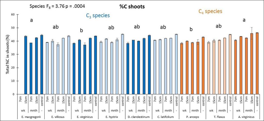
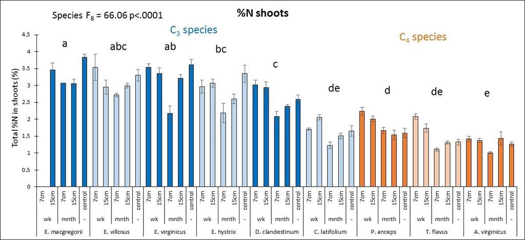
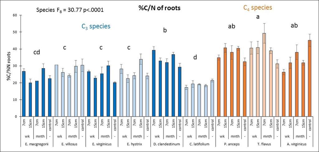
128 113

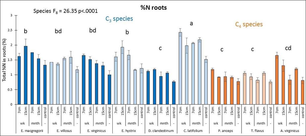
129 114

130 Figure 4.6: Microscopic variables with treatment means (±SE) for each species. The species are listed on the x-axis in order of their flowering times. F and p values for the overall species comparisons over all treatments are included with different letters signifying significant differences between species overall mean (P value 0.05) determined by adhoc Tukeys. 115

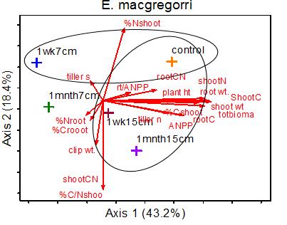
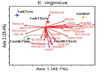
131 116

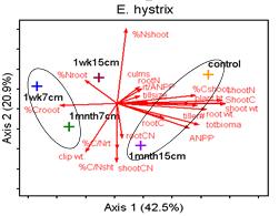
132 117

133 Figure 4.7: PCA results for each species using all traits and grouped by treatment. The circles represent the treatment means that are not significantly different in pairwise comparisons using MRPP (p<.025). The percent of variance explained for each axis is reported. 118