Accepted Manuscript. Boolean Modeling of Biological Regulatory Networks: A Methodology Tutorial. Assieh Saadatpour, Réka Albert

Transcription

1 Accepted Manuscript Boolean Modeling of Biological Regulatory Networks: A Methodology Tutorial Assieh Saadatpour, Réka Albert PII: S (12) DOI: Reference: YMETH 3019 To appear in: Methods Please cite this article as: A. Saadatpour, R. Albert, Boolean Modeling of Biological Regulatory Networks: A Methodology Tutorial, Methods (2012), doi: This is a PDF file of an unedited manuscript that has been accepted for publication. As a service to our customers we are providing this early version of the manuscript. The manuscript will undergo copyediting, typesetting, and review of the resulting proof before it is published in its final form. Please note that during the production process errors may be discovered which could affect the content, and all legal disclaimers that apply to the journal pertain.

2 Boolean Modeling of Biological Regulatory Networks: A Methodology Tutorial Assieh Saadatpour a and Réka Albert b* a Department of Mathematics, The Pennsylvania State University, University Park, PA 16802, USA b Department of Physics, The Pennsylvania State University, University Park, PA 16802, USA * Corresponding author ralbert@phys.psu.edu Address: 104 Davey Laboratory, The Pennsylvania State University, University Park, PA 16802, USA Tel.: Fax: addresses: AS: saadat@math.psu.edu RA: ralbert@phys.psu.edu

3 Abstract Given the complexity and interactive nature of biological systems, constructing informative and coherent network models of these systems and subsequently developing efficient approaches to analyze the assembled networks is of immense importance. The combination of network analysis and dynamic modeling enables one to investigate the behavior of the underlying system as a whole and to make experimentally testable predictions for less-understood aspects of the processes involved. In this paper, we present a tutorial on the fundamental steps for Boolean modeling of biological regulatory networks. We demonstrate how to infer a Boolean network model from the available experimental data, analyze the network using graph-theoretical measures, and convert it into a predictive dynamic model. For each step, the pitfalls one may encounter and possible ways to circumvent them are also discussed. We illustrate these steps on a toy network as well as in the context of the Drosophila melanogaster segment polarity gene network. Keywords: Biological regulatory networks, Boolean models, Structural analysis, Dynamic analysis, Drosophila segment polarity gene network Highlights The basic steps for Boolean modeling of regulatory networks are presented Inference of a Boolean network model from the available experimental data is described Structural analysis of the inferred network using graph measures is explained Different Boolean dynamic approaches are described The obstacles one may encounter in the above steps are discussed 1

4 1. Introduction Recent advances in high-throughput techniques have led to a tremendous growth in the amount and type of biological data that reflect various biological interactions at different levels. Any cell responds to its environmental stimuli through a coordinated sequence of biological processes that includes interactions and regulation at the signal transduction, gene, protein or metabolism level [1]. For example, at the gene level, transcriptional regulatory proteins regulate the activity of their own or of other genes, i.e. induce or repress the transcription from the respective genes, leading to an increase or a decrease in the amount of the expressed mrna transcript. This in turn changes the concentrations of the corresponding proteins and subsequently leads to a new state, or possibly a new behavior of the cell. Therefore all genes and their products (i.e., proteins) form a complex web of interactions, in which each component can have a positive or negative effect on the activity of other components. The interactions at the protein level arise from the fact that proteins can form complexes to enable additional functionalities or they can be involved in posttranslational modification of other proteins. Given the large number of components (i.e., thousands of genes, proteins and metabolites) and complex interactions among them, network modeling can serve as a powerful tool for coherent representation of the whole system in a unified template. In network modeling the components of the system are described by nodes (vertices), whereas the interactions and processes among them are denoted by edges (links). Edges in the network can be directed according to the orientation of mass transfer or information propagation. In addition, the interaction types can be signified with a positive or negative sign representing activation or inhibition, respectively. The aforementioned processes at different levels can be represented in the form of signal transduction networks [2,3], gene regulatory networks [4,5], protein-protein interaction networks [6,7], and metabolic networks [8,9], respectively. In particular, the nodes of the gene regulatory networks, in their most general form, consist of genes, mrnas, and proteins, and the edges denote transcription, translation, transcriptional regulation or proteinprotein interactions. Considering the myriad of components available inside a cell, we may deal with enormously complicated networks of interactions. Deciphering the structure and dynamics of these networks is the first step towards understanding the overall behavior of the cell. The network representation provides a backbone for structural analysis and dynamic modeling of the underlying biological system. Structural analysis includes the use of graph-theoretical measures, such as centrality measures and shortest paths, to extract information on the heterogeneity and organization of the network [10]. Dynamic models reflect the fact that the nodes of the network are molecular species, and describe how the population levels of these species change over time. Dynamic modeling approaches are divided into two major categorizes, namely continuous or discrete, according to the description of nodes states. Continuous models, usually described as a set of differential equations, are the most relevant strategy to capture the dynamical nature of biological systems. However, the use of these models is hampered by the scarcity of the kinetic details of the interactions in all but a handful of extensively studied pathways. On the 2

5 other hand, discrete models, such as finite state logical models [11,12], Boolean models [13,14], and Petri nets [15,16], provide a qualitative description that requires no or few parameters. The class of piece-wise linear differential equation (hybrid) models [17,18], bridges the gap between continuous and discrete models by characterizing each node by two variables, a continuous concentration and a discrete activity. These models meld the logical description of the regulatory relationships with a linear concentration decay. Which model to select depends on the level of quantitative details of the available experimental data: continuous models can be employed when sufficient kinetic information is available, discrete models are best suited for less-characterized systems with no kinetic details, and hybrid models can be used when partial information on the kinetic parameters is available. The focus of this tutorial is on Boolean models, which were first introduced by S. Kauffman [19] and R. Thomas [20] for modeling gene regulatory networks. In these models each node can have only two qualitative values; 0 (OFF) and 1 (ON). The OFF state refers to a below-threshold concentration or activity, which is insufficient to initiate downstream processes, and the ON state is an above-threshold concentration or activity. Although the concentration of components in biological systems changes continuously over time, the input-output curves of the regulatory interactions are often sigmoidal and can be well estimated by step-functions [14], thereby providing an ample justification for the use of Boolean models. Notably, these models have been successfully applied in modeling various biological systems such as the segment polarity gene network in Drosophila melanogaster [21,22,23], flower morphogenesis in Arabidopsis thaliana [24], cortical area development in mammalian brain [25], the cell cycle regulatory network in Saccharomyces cerevisiae (budding yeast) [26] and Schizosaccharomyces Pombe (fission yeast) [27], mammalian cell cycle [28], glucose repression signaling pathways in Saccharomyces cerevisiae [29], mammalian immune response to bacteria [30], T cell receptor signaling [31], phospholipase C-coupled calcium signaling [32], abscisic acid signaling network in plants [33], as well as a T cell survival network in humans [34]. In this paper, we provide a tutorial on the basic steps of Boolean modeling of biological regulatory networks with a focus on gene regulatory networks. However, the methods are general enough to be applied to signal transduction networks as well, and indeed they have been applied successfully [29,31,32,33,34]. We demonstrate how to infer a Boolean network from the available experimental data, analyze it using graphtheoretical measures, and convert it into a predictive dynamic model. For each step, the decisions and revisions that may need to be made are described. These steps are demonstrated for a toy network and in the context of the well-studied Drosophila segment polarity gene network, which we describe next. 2. Drosophila segment polarity gene network The body of the fruit fly Drosophila melanogaster, like in other arthropods, is composed of segments. A single-celled egg is developed into a multi-cellular embryo with 14 segments through a hierarchical cascade of genetic interactions involving more than 40 genes [35]. The successive transient expression of the gap and pair-rule genes 3

6 from maternal morphogens creates a prepattern of the parasegments (the embryonic counterparts of the segments) and initiates the expression of the segment polarity genes. These genes, which are expressed throughout the life of the fruit fly, stabilize the pattern, define narrow boundaries between the parasegments, and contribute to subsequent developmental processes [35,36]. These genes have a periodic spatial expression pattern wherein their mrna is expressed (has a high concentration) in certain cells, and not expressed (has a very low concentration) in other cells. The main segment polarity genes include engrailed (en), wingless (wg), hedgehog (hh), patched (ptc), cubitus interruptus (ci) and sloppy paired (slp) (see e.g. [37,38,39]), which encode for their corresponding proteins denoted by EN, WG, HH, PTC, CI, and SLP. Two additional proteins, which are cleaved from CI, are also involved: a transcriptional activator (CIA) and a transcriptional repressor (CIR). The segment polarity genes refine and maintain their expression through a network of intra- and inter-cellular regulatory interactions, which is referred to as the Drosophila segment polarity gene network [21,40]. This network has been extensively studied using continuous [40,41,42,43], Boolean [21,22,44,45], as well as hybrid [23,46] approaches. The primary goal of these models were to capture the spatially resolved expression of the segment polarity genes, starting from an initial condition corresponding to the initial prepattern of the genes, and ending at a steady state that corresponds to the known sustained pattern of the genes. The models also examined how this process changes in the presence of transient or permanent perturbations. von Dassow et al [40] proposed the first model for this network: a continuous model containing 13 differential equations and 48 unknown kinetic parameters. Their results suggested that the network s topology has an essential impact on the robustness of the model. This idea was further supported using Boolean dynamic models [21,22]. In the following section, we describe Boolean modeling of biological regulatory networks in a step-by-step fashion with illustrations from the Drosophila segment polarity gene network. 3. Boolean models A Boolean network model provides a qualitative representation of a system wherein each node can take two possible values denoted by 1 (ON) or 0 (OFF). This indicates, for example, that a gene is expressed or not expressed, a transcription factor is active or inactive, and a molecule s concentration is above or below a certain threshold. This binary value represents the state of a node. In Boolean models, the future state of a node is determined based on a logic statement on the current states of its regulators. This statement, called a Boolean rule (function), is usually expressed via the logic operators AND, OR, and NOT. A simple network containing three nodes along with the Boolean rules that express the regulation among the nodes is given in Figure Network inference Reconstruction of a network structure for a biological regulatory system consists of integrating information about the components involved in the system and their 4

7 interactions from either gene expression (e.g. microarray) data or causal experimental observations Inference of the nodes of the network As currently it is not possible to comprehensively model the dynamics of genomewide regulatory networks, the model is usually confined to target a single behavior or outcome, e.g. parasegment formation in Drosophila melanogaster [21,40], or differentiation of T cells [47,48]. The aim of this focused model is to include all the genes and gene products involved in the targeted outcome or behavior. The list of components to include usually starts from a core set known from the literature, and it expands as additional information is included. For example, large-scale gene expression data can be used to identify which genes are differentially expressed over the examined conditions, thus indicating that these genes may be associated with the behavior of interest [49,50,51]. In addition, new nodes for the regulatory network can be identified using causal experiments, where modulation of an already known component of the network leads to variations in expression/concentration of a gene/protein, implying that the gene/protein should be added to the network [52] Inference of the edges of the network Once the nodes of the network are identified, the next step is to infer the edges connecting these nodes (i.e., interactions among the components). Information on the edges of a regulatory network can be obtained from either gene expression data [53,54,55,56,57,58,59,60,61] or causal experiments [62]. Inference of edges from gene expression data is achieved using probabilistic, deterministic, or probabilisticdeterministic hybrid methods [63]. Among the probabilistic approaches are Bayesian network methods [54,55], which detect a directed, acyclic (feedback loop free) graph, along with a set of joint probability distributions describing the causal relationships among the components. Dynamic Bayesian networks allow the inclusion of cyclic regulatory pathways in the inferred network [61]. Deterministic model-driven approaches, including continuous [56,57] and discrete methods [58,59], relate the rate of change in the expression level of a given gene to that of other genes using a set of differential or logic equations. Solving these equations results in the identification of potential regulatory relationships that can best reproduce the observed expression data. Probabilistic-deterministic hybrid methods, such as probabilistic Boolean networks [60], take into account stochastic fluctuations in gene expression levels by incorporating uncertainty in the designated dependency relationships. There are three major types of causal experimental evidence from which information on edges of a network can be extracted [62]: 1) biochemical evidence of transcription factor-gene interactions, enzymatic activity or protein-protein interactions which indicate direct interaction between two components; 2) genetic evidence of the effect of the mutation of a particular component on another component; this evidence leads to an indirect causal relationship between the two components; or 3) pharmacological evidence of the effect of exogenous treatment of a particular component on another component; 5

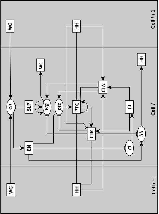
8 this evidence also leads to an indirect causal relationship between the two components. The integration of the indirect causal evidence is often challenging and non-intuitive, as each such apparently pairwise relationship may in fact reflect a set of adjacent edges (a path) in the network, and it may involve other, known or unknown nodes. Fortunately algorithmic approaches exist and have been implemented in the software package NET- SYNTHESIS [64], a regulatory network inference and simplification tool, which generates the sparsest network consistent with the given causal evidence. In some cases, one may need to perform manual curation of the output of the software to find the most realistic network corresponding to the available experimental observations [34] Network visualization After the nodes and edges of the network were identified, one can assemble a network corresponding to the regulatory system of interest to get a big picture of the whole system and its interactions. Several software packages are available for network visualization and analysis including the yed Graph Editor [65], Graphviz [66], Cytoscape [67,68], and Pajek [69] Inference of the Drosophila segment polarity network The interaction network corresponding to the segment polarity genes in Drosophila was constructed based on qualitative experimental data (generally of genetic nature) on causal relationships among the genes [21,40]. As mentioned earlier, von Dassow et al [40] constructed the first network for the segment polarity genes in Drosophila containing five genes (en, wg, ptc, ci, and hh) and their proteins, and modeled it using a continuous approach. Their initial choice of the network topology was not able to reproduce the observed expression patterns of the genes. However, adding two new interactions (an activating edge from WG to wg as well as an inhibitory edge from CIR to en) to the network restored consistency with known robust patterns even in the presence of large variations in the kinetic parameters. The authors of the first Boolean model of this network decided to not include the putative inhibitory edge from CIR to en as no evidence was found in the literature to support the presence of this edge in the network and they also incorporated the wg auto-regulation in a weaker form [21]. Other extensions of this reconstructed network includes addition of an inhibitory edge from EN to ptc as well as a new node called Sloppy Paired (SLP) with its respective edges, all supported by experimental observations [21]. This network was subsequently refined further by Chaves et al [22] as depicted in Figure 2. This figure represents intra- and inter-cellular interactions of a cell and its two neighbors. When expression of the segment polarity genes begins, a given gene is expressed in every fourth cell [21]. Thus one can focus on a single parasegment of four cells and impose periodic boundary conditions on the ends. There are 13 components per cell, thus the total number of nodes in the model is 4 13=52. 6

9 3.2. Constructing the Boolean rules Having assembled the network, the next step is to construct the Boolean rules based on the relevant literature. If a node has only one regulator, then a single variable, usually denoted by the label of the regulator, appears in its Boolean rule. This variable is combined with a NOT operator if the regulator is an inhibitor. For example, node A in Figure 1A is inhibited by node C, resulting in the Boolean rule A*=NOT C, where the asterisk signifies the future state of node A. When a node has multiple regulators, the OR operator is used if any of the regulators can activate the node, and the AND operator is used if co-expression of all of them is required for successful activation of the node. For example, in the case of node B in Figure 1A the rule B*=A AND C expresses that both A and C need to be active (ON) in order for B to be able to turn ON. When constructing the Boolean rules, one may encounter difficulties in deciding whether to use an AND or OR operator in a rule wherein a node is controlled by more than one regulator. For example, node B in Figure 1 is regulated by A and C. How can one determine, in a real situation, if activation of both A and C, or only one of them, is required for the activation of B? If there is experimental evidence that knocking out either A or C leads to the absence of B, then AND should be used. Conversely, if there is evidence that only simultaneous knockout of A and C would inactivate B, then OR should be used. When no such information is available, the OR operator may be used as a default, and the model can be updated once additional information is obtained. Alternatively, one can also employ probabilistic Boolean networks [60,70], which allow incorporating uncertainty in the rules by assigning different Boolean rules to a node, each with a certain probability of being selected Constructing the Boolean rules for the Drosophila segment polarity gene network In constructing the Boolean rules for this network, first some general assumptions were made: (i) inhibitors are always dominant over activators, and (ii) the state of proteins follows the state of their mrnas with a time delay. However, there are some exceptions from the latter assumption. For example, the rule for PTC allows for sustained PTC expression even if its mrna ptc decays. There are three justifying arguments for this rule. First, experimental observations support a sustained, though diminished, level of PTC in the third cell of the parasegment whereas ptc expression disappears from this cell [71]. Second, as PTC is a transmembrane receptor protein and binding to HH of the neighboring cells is the only reaction PTC participates in, it can be assumed that existing PTC levels are maintained even in the absence of ptc if there is no HH in the neighboring cells [21]. Third, allowing PTC to decay from the third cell following the decay of ptc will cause the production of CIA instead of CIR in that cell, which will then cause the abnormal expression of wg in the third cell. We also note that the expression of SLP protein is assumed to be constant. Indeed, this protein (which is a merger of two proteins with similar functions) is translated from the pair-rule gene slp, which is activated before the segment polarity genes and expressed 7

10 constitutively thereafter [72,73]. Since the translation of SLP is not affected by any nodes in the segment polarity network, it was assumed that its expression does not change. The full description of the Boolean rules is given in Table Structural analysis Structural analysis of an assembled network by means of graph-theoretical measures sheds light on the topological organization and function of the underlying biological system. These measures range from local to global topological measures, which provide information on individual nodes/edges or the whole network, respectively. The most often used measures include connectivity (such as distance) and centrality (such as node degree or betweenness centrality) measures. The Python library NetworkX [74] offers tools for such analysis. From a graph theory standpoint, a path is a sequence of adjacent edges in the network. The number of edges on the shortest path connecting two given nodes is called the distance between the two nodes. For example, the distance between A and B in Figure 1A is 1, while the distance between B and A is infinity as there is no path from B to A. A network is connected (or strongly connected in the directed case) if there is a path (or two directed paths of opposite orientations in the directed case) between every pair of nodes. If a network is not (strongly) connected, it is informative to identify (strongly) connected components (or sub-graphs) of the network. In directed graphs, each strongly connected component (SCC) has an in-component (nodes that can reach the SCC) and outcomponent (nodes that can be reached from the SCC). For example, nodes A and C in Figure 1A form an SCC having node B in its out-component. It was reported that the transcriptional regulatory networks have no or only small SCCs (e.g. three-node feedback loops) [75,76], whereas a large SCC was observed in metabolic [77] and signaling [78] networks. Centrality measures describe the importance of individual nodes in the network. The simplest of such measures is the node degree, which quantifies the number of edges connected to each node. For directed networks, the in- and out-degree of a node is defined as the number of edges coming into or going out of the node, respectively, which collectively define the node degree. In particular, the nodes with only outgoing edges (that is, nodes with in-degree=0) are called sources and nodes with only incoming edges (out-degree=0) are sinks of the network. Such nodes indicate the initial and terminal points of flow propagation in signal transduction networks. In Figure 1A, for example, node B is a sink node. It is also useful to determine the nodes whose degree is highest among other nodes, termed hubs, whose removal can break down a network into isolated clusters [10]. The expression patterns of gene products in regulatory networks can be used to further classify hubs into permanent hubs, e.g. multi-functional transcription factors and house-keeping regulators, and transient hubs which are influential in one condition but less so in others [79]. The betweenness centrality of a node is another centrality measure, which is defined as the fraction of shortest paths between any pair of nodes passing through the given node [80]. This measure provides information on the importance of a node in mediating flow through the network. The betweenness centrality 8

11 of an edge can be defined similarly [81]. Although node degree and betweenness centrality (of a node or an edge) are local topological properties, they can be generalized to distributions over all the nodes (or edges) of the network to get insights into the heterogeneity (diversity) of node interactivity levels or of the flow propagation through the network [63]. For example, transcriptional regulatory networks tend to have a decreasing but long-tailed out-degree distribution (indicating a large heterogeneity, including the existence of transcription factors that regulate many genes) and a narrower in-degree distribution [82,83]. Besides the measures described above, it is also beneficial to identify network motifs, recurring patterns of interconnection with well-defined topologies, which form simple building blocks of the network architecture [84]. Among these motifs are feedforward and feedback loops. A three-node transcriptional feed-forward loop consists of a transcription factor X that regulates a second transcription factor Y, and both X and Y regulate gene Z [85]. Notably, such motifs are more abundant in the transcriptional regulatory networks of different organisms compared to randomized networks of the same degree distribution [84,86,87]. Feed-forward loops can carry out functions such as filtering of noisy input signals, pulse generation and response acceleration [85]. A feedback loop is a directed cycle whose sign depends on the number of negative interactions in the cycle; a positive/negative feedback loop has an even/odd number of negative interactions [14]. These motifs, as we will see in the next subsection, play a pivotal role in the dynamics of a system [14,88,89]. In the Drosophila segment polarity network given in Figure 2, the node SLP has only outgoing edges (in-degree=0), thus it is a source node in the network. All other nodes have non-zero in- and out-degrees. The two proteins CIR and CIA have the highest indegree of four as they can be activated in many ways. HH has the highest out-degree as it has three outgoing edges to each of the neighboring cells, thus affecting the future expression of six other nodes. We can also see that there are two negative feedback loops between ptc, PTC, and CIR as well as between ptc, PTC, and CIA. We also note that there is a way of incorporating the Boolean rules into the structure of a network by introducing a complementary node for any node whose negated expression (by the NOT operator) appears in the rules as well as a composite node for any combination of the nodes connected by the AND operator [21]. Although this expansion of the network increases the number of nodes, it has the benefit of having only one edge type, that is, all the edges now indicate activation. The expanded network of the segment polarity genes provided important insights into the identification of coexpressed genes [21]. For example, it showed that the cells expressing en and hh never express wg, ptc, or ci, a well-known polarization that is the basis for the name segment polarity genes [36]. In a recent study [90], the idea of expanding the network combined with consideration of the cascading effects of a node s removal was utilized to identify essential components of signal transduction networks. In that study, the concept of elementary signaling mode, defined as the minimal set of nodes that can perform signal transduction independently, was also introduced; this is an adaptation of the path concept to networks exhibiting combinatorial regulation. Although this method was primarily 9

12 used for signal transduction networks, it can be adapted for evaluating the importance of genes in gene regulatory networks by considering the connectivity of the whole network instead of the connectivity from source to sink nodes [90]. It should be noted that among the graph-theoretical measures described above, only the latter one requires the knowledge of the Boolean rules, analysis of the other measures only needs the knowledge of nodes and edges of the network Dynamic analysis Time implementation In order to convert a static network representation into a dynamic model, one first needs to decide how to implement time. In Boolean models, time is an implicit variable and can be implemented via synchronous or asynchronous update algorithms. Synchronous models assume similar timescales for all the processes involved in a system, and are implemented by updating all the nodes states simultaneously [13]. More precisely, the state of node i at time step t+1, denoted by x i (t+1), is determined based on the state of its regulators at the t th time step: x i (t +1) = f i (x i1 (t), x i2 (t),..., x im i (t)) (1) where f i is the Boolean rule for node i and x i j s, 1 j m i, are the states of its regulators. Although the simplicity and computational efficiency of synchronous models is attractive, they cannot describe well the biological systems that include processes at multiple levels, e.g. mrna, protein, and post-translational levels, because the timescales of these processes ranges from fractions of a second to hours [3]. To overcome this limitation, asynchronous models have been developed wherein the nodes are updated based on their individual timescales [14]. Different asynchronous algorithms have been proposed so far, including the random order asynchronous [22,91], deterministic asynchronous [23], and general asynchronous [91] algorithms. In the random order asynchronous algorithm, at each time step a random permutation of the nodes is selected and the nodes are updated in that order [22]. In this case, x i (t+1) is determined according to the most recent updated state of the regulators of node i: x i (t +1) = f i (x i 1 (τ i1 ),..., x im i (τ im i )) (2) where τ i j {t,t +1}. Indeed τ i j = t +1 if the position of regulator j is before node i in the permutation, and τ i j = t otherwise. In the deterministic asynchronous framework, each node has a pre-selected (either based on a priori knowledge or randomly chosen from a uniform distribution) time unit, γ i, and is updated at positive multiples of that unit [23]: x i (t +1) = f i (x i 1 (t),..., x imi (t)) if t +1 = kγ i, for some k N x i (t) otherwise (3) 10

13 In the general asynchronous framework, at each time step a randomly selected node is updated [91,92]. A recent study provides a comparison of these three asynchronous methods applied on the same biological system [93] Attractor analysis By updating the state of the nodes according to the synchronous or asynchronous algorithms, one can obtain the state of the whole system at each time step, which is expressed by a vector whose i th element represents the state of node i at that time step. We note that the Boolean model of a network with n nodes has a total of 2 n states. These states and the allowed transitions among them form the state transition graph of the system. Starting from an initial state in the state transition graph and iteratively updating the state of the nodes, the state of the system evolves over time and following a trajectory of states, it eventually settles into an attractor. Attractors, which describe the long-time behavior of a system, fall into two groups: fixed points (steady states), wherein the state of the system does not change, and complex attractors, wherein the system oscillates among a set of states. As fixed points of a system are time independent, they are the same for both synchronous and asynchronous models. To obtain the fixed points, one can remove the time dependency from the Boolean rules and solve the resulting set of equations. Complex attractors are different in synchronous and asynchronous models: in synchronous models, the system regularly oscillates among a set of states, called a limit cycle, whereas in asynchronous models the system may oscillate irregularly among a set of states which form the SCC of the state transition graph with an empty out-component. For each attractor, the set of states that can reach that attractor are called the basin of attraction of that attractor. Figure 3 represents the state transition graph of the network given in Figure 1 using synchronous and random order asynchronous models. In both models, the state 001 and 100 are the fixed points. The synchronous model also has a limit cycle of period two containing the states 010 and 101 (period of a limit cycle is the number of states in the cycle), which is absent from the asynchronous model. Indeed, synchronous models may exhibit limit cycles unconfirmed by the corresponding continuous or asynchronous models [28,93,94]. We also note that the fixed points can be obtained analytically by solving the Boolean equations given in Figure 1B independent of time. Indeed, substituting A=NOT C into the second and third equations results in B=0 and C=C. The latter expression implies that C can be 0 or 1, and as a result A can be 1 or 0, respectively. Therefore the two fixed points (001, and 100) are obtained analytically as well. By comparing the state transition graphs given in Figures 3A and 3B, we see that in the state transition graph of the synchronous model, each state has a unique successor, which is not the case in the asynchronous model. Consequently, each attractor in the state transition graph of the synchronous model has a unique basin of attraction, whereas the basin of attraction of different attractors in (random) asynchronous models may overlap. For example, states 000, 010, 101, and 111 in Figure 3B are in the basins of attraction of both fixed points. 11

14 Absorption times and absorption probabilities A random asynchronous model can be characterized by a Markov chain for which each entry of its transition matrix, p ij, denotes the probability of a transition from state i to state j, 0 i, j 2 n 1 (decimal representation of the binary numbers). If a system has at least one fixed point and it is possible to reach a fixed point from each transient state, then starting from an initial state, the expected number of time steps to be absorbed into one of the fixed points (absorption time) as well as the probability to reach each fixed point (absorption probability) can be computed using the analysis of the transition matrix (see e.g. [95]). For example, the transition matrix corresponding to the state transition graph given in Figure 3B is as follows where the probabilities represent the fractions of the total number of permutations transforming one state to another: 0 1/ / / / P = /3 0 1/6 1/3 0 1/ /3 0 1/6 1/3 0 1/6 0 By a rearrangement of the states, the matrix P can be partitioned as P = Q R 0 I, where Q denotes the transient states, I is an identity matrix, and R is the remaining part. When the chain starts from the transient state i, the expected number of time steps for the chain to be absorbed into one of the fixed points is obtained by summing up the entries of the i th row of the matrix (I Q) 1, where I is the identity matrix of the same size as Q. In addition, the probability to reach each fixed point from the transient state i is given by the i th row of the matrix (I Q) 1 R [95]. The absorption times and probabilities for the state transition graph of Figure 3B are given in Table 2. As we can see, the absorption times from states 101 and 111 are longer than the other states as they have multiple ways to reach the fixed points. Furthermore, except for two cases that converge to only one of the fixed points, all other states reach the two fixed points with equal probabilities Network reduction As the size of the state transition graph of a Boolean network is an exponential function of the number of nodes in the network, it is difficult to map the whole state transition graph for large networks. In such cases, one can sample over a large set of initial states [96] or take advantage of the available network reduction techniques to simplify the network while preserving its essential dynamical properties [93,97,98]. For example, we recently proposed a network reduction method and successfully applied it to gain insights into the dynamic behaviors of the drought response in plants and the T-LGL leukemia signaling network in humans [93,99]. This method (i) determines and eliminates the nodes whose states stabilized due to their regulation and irrespective of the 12

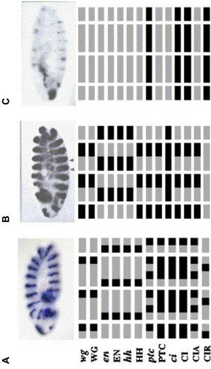
15 update method or initial condition; and (ii) iteratively removes simple mediator nodes such as the ones with in- and out-degree of one. This reduction method enabled us to identify, for example, attractors of the unperturbed and perturbed models of the T-LGL leukemia signaling network and to analyze their basins of attraction, thereby predicting novel candidate therapeutic targets for the disease [99] Effect of the feedback loops The structure of a network plays a determinant role in its dynamics. For example, it has been conjectured that the presence of positive feedback loops in the network is necessary for multi-stability (having multiple steady states), while negative feedback loops are necessary for sustained oscillations [89]. This conjecture was proven correct in several continuous [100,101,102,103] and discrete [104,105] frameworks. In the network of Figure 1A, for example, there is a positive feedback loop between the nodes A and C. Thus, observing multiple fixed points was expected Software packages for dynamic simulations Several software resources can be employed for simulation and dynamic analysis of Boolean models such as BooleanNet [106], BoolNet [107], GINsim [108], CellNetAnalyzer [109,110], SimBoolNet [111], and ADAM [112], some of which can be also used for structural analysis of the network. The state transition graphs in Figure 3 were generated using BooleanNet Dynamic analysis of the Drosophila segment polarity gene network Now we illustrate how the described dynamic methods were applied in the context of the Drosophila segment polarity gene network. The segment polarity genes maintain the parasegment borders and later the polarity of the segment in stages 8-11 of the embryonic development [36]. As the Boolean dynamic model of this network was intended to describe the effect of the segment polarity genes in maintaining the parasegment borders, the patterns of these genes formed before stage 8 was considered as the initial state of the system [21]. This initial state includes a two-cell-wide SLP stripe in the posterior (toward the tail) half [72], a single-cell-wide wg stripe in the most posterior part [35], single-cellwide en and hh stripes in the most anterior (toward the head) part [35,113], and ci and ptc expressed in the posterior three-fourths [35,71,114]. Since the proteins are translated after the mrnas are transcribed, it was assumed that the proteins are not expressed (OFF) in the initial state [21]. Starting from the above initial state, the synchronous model of the system reached the wild-type fixed point, in agreement with the experimentally known results, after six time steps [21]. Removing the time dependencies from the Boolean rules in Table 1 and solving the resulting set of Boolean equations, as it was done for the simple example of Figure 1, results in ten solutions, six of which being distinct fixed points as summarized in Table 3, and the rest are minor variations of the previous six [21]. Three distinct fixed points were observed experimentally, corresponding to the wild-type state and two states 13

16 (with either broad stripes or no stripes) observed in knockout and over-expression experiments, as depicted in Figure 4. The existence of the additional fixed points suggests that, for suitable initial conditions, this network can produce patterns beyond those required in Drosophila embryogenesis [21]. Estimating the size of the basins of attraction of each fixed point was achieved by fixing the state of all but one as in that fixed point and determining how many of such states reach that particular fixed point. This procedure was repeated for all the initial states wherein the expression of pairs and triplets of nodes is different from that fixed point. After extrapolation it was estimated that only a small fraction of the total initial states reach the wild-type fixed point whereas the majority of the states reach the fixed point with broad stripes. Introducing time variability into the model using asynchronous dynamic frameworks revealed further insights into the development of gene expression patterns. For example, the random asynchronous model of the system showed that in the course of a large number of simulations that start from the wild type initial condition but use different random node permutations, more than half of the simulations lead to the wild-type fixed point but a considerable percentage results in an infeasible final state, for example the non-segmented or broad-striped pattern [22]. This is indicative of the fragility of the wild-type pattern with respect to unbounded variability of the synthesis and decay timescales. It was also found that the divergence from the wild type is due to a transient CIA/CIR imbalance in the posterior half of the parasegment, thus predicting that perturbations of the post-translational modification of Cubitus Interruptus can have as severe effects as mutations [22]. Interestingly, introducing a single realistic constraint, i.e., a timescale separation between protein-level processes and mrna-level processes, resulted in having only the wild-type (with a frequency of 87.5%) and broad striped (with a frequency of 12.5%) fixed points. A similar timescale separation in the deterministic asynchronous version yielded a convergence to the wild-type fixed point with a frequency of 93% or more [23]. Analysis of the absorption times for the random order asynchronous model of this network revealed the fast convergence to the wild-type pattern (with an expected time of 4 steps), contrasted with the long and oscillation-strewn path toward the broad striped pattern (with an expected time of 15 steps) [22]. Taken together, these results suggest that the system s dynamical trajectory is robust even in the presence of considerable variability in timescales Validity of the reconstructed model To assess the validity of a reconstructed model, one needs to check if the known experimental observations can be replicated by the dynamic analysis. Therefore, if there is experimental evidence for a certain behavior of a system, which cannot be reproduced by the dynamic model, then the network model and/or the Boolean rules should be revised. To this end, one can, for example, change the rules with uncertainties in them e.g. those for which it was not clear whether to use an OR or AND operator. Since the Boolean model of the Drosophila segment polarity gene network reproduces the available experimental observations quite well, it suggests that the structure of the network reasonably represents the core features of the underlying biological system. Once new information on the involvement of additional nodes/edges in a synthesized 14

17 network becomes available, they can be incorporated into the model. For example, after the reconstruction of the segment polarity gene network it was observed experimentally that the EN protein inhibits slp transcription [115]. Subsequently, to incorporate this experimental observation into the Boolean model, the following rule was suggested for slp and SLP [23]: 0 if i {1,2} RX i * = 1 if i {3,4} slp i * = RX i AND NOT EN i SLP i * = slp i where RX represents a combination of regulation by the pair-rule genes responsible for the establishment of slp. Considering the wild-type initial states for slp and SLP, it was proven that this new rule results in constant patterns for the two nodes and accordingly the same results as in the previous models [23]. In a later model, the rule was refined further to incorporate the feedback of the segment polarity network on SLP without the need of introducing the new node RX [46] Robustness of the reconstructed model In order to assess the robustness of the reconstructed model one can perform a perturbation analysis on the network structure and Boolean rules, or on the nodes states. For the former, the robustness can be examined through, for example, randomly adding an edge between two components or interchanging OR and AND operators in a rule. For the latter, one can study the effect of knockout or over-expression mutations by fixing the state of a node at 0 or 1, respectively. This analysis can be performed on a particular initial state of the system or on the attractors. For example, knocking out en, wg, or hh in the wild-type initial state of the Drosophila segment polarity gene network in the synchronous model led to the fixed point with no segmentation (see Table 3), while ptc knockout or several over-expressed initial states resulted in the broad-striped pattern, in agreement with numerous experimental observations [21]. One of the interesting predictions of this analysis was the importance of the wg prepattern as it was found that an initial condition with no cell expressing wg or WG led to the same non-segmented attractor as a wg knockout. Several other researchers also studied the effect of perturbations in the nodes states or in the Boolean rules on the attractors of the segment polarity gene network [44,45,116]. For example, Subramanian and Gadgil [45] studied the robustness of the synchronous model of this system under transient perturbations in the nodes states. By flipping the state(s) of one or multiple nodes in the wild-type fixed point for a short period of time, they identified critical nodes, such as wg in the first and third cells or en and hh in the second and forth cells of the parasegment and their proteins, whose state changes lead the system away from this fixed point [45]. For systems with cell-to-cell interactions robustness to changes in the number of cells can also be studied. This has been done in the Drosophila segment polarity gene network using the synchronous Boolean as well as hybrid frameworks and led to the 15

18 conclusion that rounds of cell division do not disrupt the pattern of the segment polarity genes [21,46]. A model is not expected to be robust to every possible change, but fulfilling some degree of robustness reflects the adaptability of the underlying biological system under different conditions and leads to biologically testable predictions. 4. Conclusions In this tutorial we presented the basic steps of Boolean modeling of biological regulatory networks from network reconstruction to structural and dynamic analysis of the inferred network. We note that the results of Boolean models are greatly affected by the accuracy of the inferred network and its Boolean rules. Therefore, to get the most out of the model it is essential to bring to bear all the available experimental observations into the assembled network. Structural and dynamic analysis of the network can then provide insights into the topological organization and temporal behavior, respectively, of the underlying system. Such an analysis holds the promise of new predictions which can guide future experimental studies, thus leading to further model refinements. Since Boolean models are parameter free, they serve as a suitable starting point for modeling poorly characterized systems, especially large-scale regulatory networks, to gain a coarse-grained insight into the unknown facets of such systems. In addition, one can incorporate certain quantitative details on the timescales (e.g. the relative rates of two processes) in Boolean models by considering priority classes either in the order of updates [22,28] or in the probabilities of the node updates [117]. Furthermore, performing a large number of Boolean dynamic simulations and obtaining the fraction of simulations that have a certain state results in a semi-quantitative curve [34]. Nonetheless, it should be noted that Boolean models cannot capture fine details of the underlying biological system. For example, negative feedback loops often generate oscillations in Boolean models (especially synchronous ones), but in continous models they can be a source of homeostasis [118] or excitation-adaptation behavior [85] as well. In addition, infinitesimal perturbation analysis cannot be achived in standard (synchronous/asycnronous) Boolean models as they only allow the extreme case of reversing a node s state [119]. In such situatitons if partial quantitative and/or kinetic information about the biological processes involved in the system is available, one can take advantage of alternative modeling strategies, such as autonomous Boolean networks [120,121] or hybrid models [18,23,122,123], in which time is considered to be continous, to get further insights into such systems. Acknowledgements The authors were supported by the National Science Foundation (Grant# CCF ). 16

19 References 1. Palsson BØ (2006) Systems Biology: Preperties of Reconstructed Networks. New York: Cambridge University Press. 2. Kestler HA, Wawra C, Kracher B, Kuhl M (2008) Network modeling of signal transduction: establishing the global view. Bioessays 30: Papin JA, Hunter T, Palsson BØ, Subramaniam S (2005) Reconstruction of cellular signalling networks and analysis of their properties. Nat Rev Mol Cell Biol 6: Karlebach G, Shamir R (2008) Modelling and analysis of gene regulatory networks. Nat Rev Mol Cell Biol 9: Lee TI, Rinaldi NJ, Robert F, Odom DT, Bar-Joseph Z, et al. (2002) Transcriptional regulatory networks in Saccharomyces cerevisiae. Science 298: Cho S, Park SG, Lee DH, Park BC (2004) Protein-protein interaction networks: from interactions to networks. J Biochem Mol Biol 37: Pellegrini M, Haynor D, Johnson JM (2004) Protein interaction networks. Expert Rev Proteomics 1: Duarte NC, Becker SA, Jamshidi N, Thiele I, Mo ML, et al. (2007) Global reconstruction of the human metabolic network based on genomic and bibliomic data. Proc Natl Acad Sci U S A 104: Hatzimanikatis V, Li C, Ionita JA, Broadbelt LJ (2004) Metabolic networks: enzyme function and metabolite structure. Curr Opin Struct Biol 14: Albert R, Barabasi AL (2002) Statistical mechanics of complex networks. Reviews of Modern Physics 74: Sanchez L, van Helden J, Thieffry D (1997) Establishement of the dorso-ventral pattern during embryonic development of Drosophila melanogasater: a logical analysis. J Theor Biol 189: Sanchez L, Thieffry D (2001) A logical analysis of the Drosophila gap-gene system. J Theor Biol 211: Kauffman SA (1993) Origins of order: self-organization and selection in evolution. New York: Oxford Univ. Press. 14. Thomas R, D'Ari R (1990) Biological Feedback. Boca Raton: CRC Press. 15. Sackmann A, Heiner M, Koch I (2006) Application of Petri net based analysis techniques to signal transduction pathways. BMC Bioinformatics 7: Chaouiya C (2007) Petri net modelling of biological networks. Brief Bioinform 8: Glass L (1975) Classification of biological networks by their qualitative dynamics. J Theor Biol 54: Glass L (1975) Combinatorial and topological methods in nonlinear chemical kinetics. J Chem Phys 63: Kauffman SA (1969) Metabolic stability and epigenesis in randomly constructed genetic nets. J Theor Biol 22: Thomas R (1973) Boolean formalization of genetic control circuits. J Theor Biol 42:

20 21. Albert R, Othmer HG (2003) The topology of the regulatory interactions predicts the expression pattern of the segment polarity genes in Drosophila melanogaster. J Theor Biol 223: Chaves M, Albert R, Sontag ED (2005) Robustness and fragility of Boolean models for genetic regulatory networks. J Theor Biol 235: Chaves M, Sontag ED, Albert R (2006) Methods of robustness analysis for Boolean models of gene control networks. Syst Biol (Stevenage) 153: Mendoza L, Thieffry D, Alvarez-Buylla ER (1999) Genetic control of flower morphogenesis in Arabidopsis thaliana: a logical analysis. Bioinformatics 15: Giacomantonio CE, Goodhill GJ (2010) A Boolean model of the gene regulatory network underlying Mammalian cortical area development. PLoS Comput Biol Li FT, Long T, Lu Y, Ouyang Q, Tang C (2004) The yeast cell-cycle network is robustly designed. Proceedings of the National Academy of Sciences of the United States of America 101: Davidich MI, Bornholdt S (2008) Boolean network model predicts cell cycle sequence of fission yeast. PLoS One 3: e Faure A, Naldi A, Chaouiya C, Thieffry D (2006) Dynamical analysis of a generic Boolean model for the control of the mammalian cell cycle. Bioinformatics 22: e Christensen TS, Oliveira AP, Nielsen J (2009) Reconstruction and logical modeling of glucose repression signaling pathways in Saccharomyces cerevisiae. BMC Syst Biol 3: Thakar J, Pilione M, Kirimanjeswara G, Harvill ET, Albert R (2007) Modeling systems-level regulation of host immune responses. PLoS Comput Biol 3: e Saez-Rodriguez J, Simeoni L, Lindquist JA, Hemenway R, Bommhardt U, et al. (2007) A logical model provides insights into T cell receptor signaling. PLoS Comput Biol 3: e Bhardwaj G, Wells CP, Albert R, van Rossum DB, Patterson RL (2011) Exploring phospholipase C-coupled Ca 2+ signalling networks using Boolean modelling. IET Syst Biol 5: Li S, Assmann SM, Albert R (2006) Predicting essential components of signal transduction networks: a dynamic model of guard cell abscisic acid signaling. PLoS Biol 4: e Zhang R, Shah MV, Yang J, Nyland SB, Liu X, et al. (2008) Network model of survival signaling in large granular lymphocyte leukemia. Proc Natl Acad Sci U S A 105: Hooper JE, Scott MP (1992) The molecular genetic basis of positional information in insect segments. In: Hennig W, editor. Early Embryonic Development of Animals. Berlin: Springer-Verlag. pp Wolpert L, Beddington R, Brockes J, Jessell T, Lawrence P, et al. (1998) Principles of Development. London: Current Biology Press. 37. Aza-Blanc P, Ramirez-Weber FA, Laget MP, Schwartz C, Kornberg TB (1997) Proteolysis that is inhibited by hedgehog targets Cubitus interruptus protein to the nucleus and converts it to a repressor. Cell 89:

21 38. Hooper JE, Scott MP (1989) The Drosophila patched gene encodes a putative membrane protein required for segmental patterning. Cell 59: Sanson B (2001) Generating patterns from fields of cells. Examples from Drosophila segmentation. EMBO Rep 2: von Dassow G, Meir E, Munro EM, Odell GM (2000) The segment polarity network is a robust developmental module. Nature 406: Ingolia NT (2004) Topology and robustness in the Drosophila segment polarity network. PLoS Biol 2: e Ma W, Lai L, Ouyang Q, Tang C (2006) Robustness and modular design of the Drosophila segment polarity network. Mol Syst Biol 2: von Dassow G, Odell GM (2002) Design and constraints of the Drosophila segment polarity module: robust spatial patterning emerges from intertwined cell state switches. J Exp Zool 294: Stoll G, Bischofberger M, Rougemont J, Naef F (2010) Stabilizing patterning in the Drosophila segment polarity network by selecting models in silico. Biosystems 102: Subramanian K, Gadgil C (2010) Robustness of the Drosophila segment polarity network to transient perturbations. IET Syst Biol 4: Chaves M, Albert R (2008) Studying the effect of cell division on expression patterns of the segment polarity genes. J R Soc Interface 5 Suppl 1: S Mendoza L (2006) A network model for the control of the differentiation process in Th cells. Biosystems 84: Mendoza L, Pardo F (2010) A robust model to describe the differentiation of T-helper cells. Theory Biosci 129: Kaech SM, Hemby S, Kersh E, Ahmed R (2002) Molecular and functional profiling of memory CD8 T cell differentiation. Cell 111: Lund RJ, Loytomaki M, Naumanen T, Dixon C, Chen Z, et al. (2007) Genome-wide identification of novel genes involved in early Th1 and Th2 cell differentiation. J Immunol 178: Mathur D, Danford TW, Boyer LA, Young RA, Gifford DK, et al. (2008) Analysis of the mouse embryonic stem cell regulatory networks obtained by ChIP-chip and ChIP-PET. Genome Biol 9: R Albert R, Assmann SM (2009) Discrete dynamic modeling with asynchronous update or, how to model complex systems in the absence of quantitative information. In: Belostotsky D, Totowa NJ, editors. Plant Systems Biology: Humana Press. pp Faith JJ, Hayete B, Thaden JT, Mogno I, Wierzbowski J, et al. (2007) Large-scale mapping and validation of Escherichia coli transcriptional regulation from a compendium of expression profiles. PLoS Biol 5: e Friedman N, Linial M, Nachman I, Pe'er D (2000) Using Bayesian networks to analyze expression data. J Comput Biol 7: Lewin A, Richardson S (2008) Bayesian methods for microarray data. In: Balding DJ, Bishp M, Cannings C, editors. Handbook of Statistical Genetics. Chichester, UK: John Wiley & Sons. 56. Gupta A, Varner JD, Maranas CD (2005) Large-scale inference of the transcriptional regulation of Bacillus subtilis. Computers and Chemical Engineering 29:

22 57. Gardner TS, di Bernardo D, Lorenz D, Collins JJ (2003) Inferring genetic networks and identifying compound mode of action via expression profiling. Science 301: Akutsu T, Miyano S, Kuhara S (1999) Identification of genetic networks from a small number of gene expression patterns under the Boolean network model. Pac Symp Biocomput: Ideker TE, Thorsson V, Karp RM (2000) Discovery of regulatory interactions through perturbation: inference and experimental design. Pac Symp Biocomput: Shmulevich I, Dougherty ER, Kim S, Zhang W (2002) Probabilistic Boolean Networks: a rule-based uncertainty model for gene regulatory networks. Bioinformatics 18: Kim SY, Imoto S, Miyano S (2003) Inferring gene networks from time series microarray data using dynamic Bayesian networks. Brief Bioinform 4: Albert R, DasGupta B, Dondi R, Kachalo S, Sontag E, et al. (2007) A novel method for signal transduction network inference from indirect experimental evidence. J Comput Biol 14: Christensen C, Thakar J, Albert R (2007) Systems-level insights into cellular regulation: inferring, analysing, and modelling intracellular networks. IET Syst Biol 1: Kachalo S, Zhang R, Sontag E, Albert R, DasGupta B (2008) NET-SYNTHESIS: a software for synthesis, inference and simplification of signal transduction networks. Bioinformatics 24: yed Graph Editor Ellson J, Gansner E, Koutsofios L, North SC, Woodhull G (2002) Graphviz Open source graph drawing tools. Graph Drawing. Berlin: Springer. pp Shannon P, Markiel A, Ozier O, Baliga NS, Wang JT, et al. (2003) Cytoscape: a software environment for integrated models of biomolecular interaction networks. Genome Res 13: Smoot ME, Ono K, Ruscheinski J, Wang PL, Ideker T (2011) Cytoscape 2.8: new features for data integration and network visualization. Bioinformatics 27: Batagelj V, Mrvar A (2003) Pajek - Analysis and Visualization of Large Networks. In: Jünger M, Mutzel P, editors. Graph Drawing Software. Berlin: Springer. pp Shmulevich I, Dougherty ER (2010) Probabilistic Boolean Networks: The Modeling and Control of Gene Regulatory Networks. New York: SIAM. 71. Taylor AM, Nakano Y, Mohler J, Ingham PW (1993) Contrasting distributions of patched and hedgehog proteins in the Drosophila embryo. Mech Dev 42: Cadigan KM, Grossniklaus U, Gehring WJ (1994) Localized expression of sloppy paired protein maintains the polarity of Drosophila parasegments. Genes Dev 8: Grossniklaus U, Pearson RK, Gehring WJ (1992) The Drosophila sloppy paired locus encodes two proteins involved in segmentation that show homology to mammalian transcription factors. Genes Dev 6: NetworkX 20

23 75. Ma HW, Buer J, Zeng AP (2004) Hierarchical structure and modules in the Escherichia coli transcriptional regulatory network revealed by a new top-down approach. BMC Bioinformatics 5: Sanz J, Navarro J, Arbues A, Martin C, Marijuan PC, et al. (2011) The transcriptional regulatory network of Mycobacterium tuberculosis. PLoS One 6: e Ma HW, Zeng AP (2003) The connectivity structure, giant strong component and centrality of metabolic networks. Bioinformatics 19: Ma'ayan A, Jenkins SL, Neves S, Hasseldine A, Grace E, et al. (2005) Formation of regulatory patterns during signal propagation in a Mammalian cellular network. Science 309: Luscombe NM, Babu MM, Yu H, Snyder M, Teichmann SA, et al. (2004) Genomic analysis of regulatory network dynamics reveals large topological changes. Nature 431: Freeman CL (1977) A set of measures of centrality based on betweenness. Sociometry 40: Girvan M, Newman MEJ (2002) Community structure in social and biological networks. Proc Natl Acad Sci U S A 99: Guelzim N, Bottani S, Bourgine P, Kepes F (2002) Topological and causal structure of the yeast transcriptional regulatory network. Nat Genet 31: Dobrin R, Beg QK, Barabasi AL, Oltvai ZN (2004) Aggregation of topological motifs in the Escherichia coli transcriptional regulatory network. BMC Bioinformatics 5: Milo R, Shen-Orr S, Itzkovitz S, Kashtan N, Chklovskii D, et al. (2002) Network motifs: simple building blocks of complex networks. Science 298: Alon U (2006) An Introduction to Systems Biology: Design Principles of Biological Circuits. Boca Raton, FL: Chapman & Hall/CRC. 86. Christensen C, Gupta A, Maranas CD, Albert R (2007) Large-scale inference and graph-theoretical analysis of gene-regulatory networks in B. Subtilis. Physica A 373: Shen-Orr SS, Milo R, Mangan S, Alon U (2002) Network motifs in the transcriptional regulation network of Escherichia coli. Nat Genet 31: Sontag E, Veliz-Cuba A, Laubenbacher R, Jarrah AS (2008) The effect of negative feedback loops on the dynamics of boolean networks. Biophys J 95: Thomas R (1981) On the relation between the logical structure of systems and their ability to generate multiple steady states and sustained oscillations. In: Numerical Methods in the Study of Critical Phenomena. Berlin: Springer Verlag. pp Wang RS, Albert R (2011) Elementary signaling modes predict the essentiality of signal transduction network components. BMC Syst Biol 5: Harvey I, Bossomaier T. Time out of joint: Attractors in asynchronous random Boolean networks. In: Husbands P, Harvey I, editors; 1997; Cambridge,U.K. pp Garg A, Di Cara A, Xenarios I, Mendoza L, De Micheli G (2008) Synchronous versus asynchronous modeling of gene regulatory networks. Bioinformatics 24:

24 93. Saadatpour A, Albert I, Albert R (2010) Attractor analysis of asynchronous Boolean models of signal transduction networks. J Theor Biol 266: Mochizuki A (2005) An analytical study of the number of steady states in gene regulatory networks. J Theor Biol 236: Grinstead CM, Snell JL (1997) Introduction to Probability. Providence, RI: AMS. 96. Campbell C, Yang S, Albert R, Shea K (2011) A network model for plant-pollinator community assembly. Proc Natl Acad Sci U S A 108: Naldi A, Remy E, Thieffry D, Chaouiya C (2011) Dynamically consistent reduction of logical regulatory graphs. Theoretical Computer Science 412: Veliz-Cuba A (2011) Reduction of Boolean network models. J Theor Biol 289C: Saadatpour A, Wang RS, Liao A, Liu X, Loughran TP, et al. (2011) Dynamical and structural analysis of a T cell survival network identifies novel candidate therapeutic targets for large granular lymphocyte leukemia. PLoS Comput Biol 7: e Cinquin O, Demongeot J (2002) Positive and negative feedback: striking a balance between necessary antagonists. J Theor Biol 216: Gouze JL (1998) Positive and negative circuits in dynamical systems. J Biol Syst 6: Snoussi EH (1998) Necessary Conditions for Multistationary and Stable Periodicity. Journal of Biological Systems 6: Soule C (2003) Graphic requirements for multistationarity. ComplexUs 1: Reichard A, Comet J-P (2007) Necessary conditions for multistationarity in discrete dynamical systems. Discrete Applied Mathematics 155: Remy E, Ruet P, Thieffry D (2008) Graphic requirements for multistability and attractive cycles in a Boolean dynamical framework. Advances in Applied Mathematics 41: Albert I, Thakar J, Li S, Zhang R, Albert R (2008) Boolean network simulations for life scientists. Source Code Biol Med 3: Mussel C, Hopfensitz M, Kestler HA (2010) BoolNet--an R package for generation, reconstruction and analysis of Boolean networks. Bioinformatics 26: Gonzalez AG, Naldi A, Sanchez L, Thieffry D, Chaouiya C (2006) GINsim: a software suite for the qualitative modelling, simulation and analysis of regulatory networks. Biosystems 84: Klamt S, Saez-Rodriguez J, Gilles ED (2007) Structural and functional analysis of cellular networks with CellNetAnalyzer. BMC Syst Biol 1: Klamt S, Saez-Rodriguez J, Lindquist JA, Simeoni L, Gilles ED (2006) A methodology for the structural and functional analysis of signaling and regulatory networks. BMC Bioinformatics 7: Zheng J, Zhang D, Przytycki PF, Zielinski R, Capala J, et al. (2010) SimBoolNet--a Cytoscape plugin for dynamic simulation of signaling networks. Bioinformatics 26: Hinkelmann F, Brandon M, Guang B, McNeill R, Blekherman G, et al. (2011) ADAM: analysis of discrete models of biological systems using computer algebra. BMC Bioinformatics 12:

25 113. Tabata T, Eaton S, Kornberg TB (1992) The Drosophila hedgehog gene is expressed specifically in posterior compartment cells and is a target of engrailed regulation. Genes Dev 6: Hidalgo A, Ingham P (1990) Cell patterning in the Drosophila segment: spatial regulation of the segment polarity gene patched. Development 110: Alexandre C, Vincent JP (2003) Requirements for transcriptional repression and activation by Engrailed in Drosophila embryos. Development 130: Xiao Y, Dougherty ER (2007) The impact of function perturbations in Boolean networks. Bioinformatics 23: Tournier L, Chaves M (2009) Uncovering operational interactions in genetic networks using asynchronous Boolean dynamics. J Theor Biol 260: Tyson JJ, Chen KC, Novak B (2003) Sniffers, buzzers, toggles and blinkers: dynamics of regulatory and signaling pathways in the cell. Curr Opin Cell Biol 15: Bornholdt S (2008) Boolean network models of cellular regulation: prospects and limitations. J R Soc Interface 5 Suppl 1: S Sevim V, Gong X, Socolar JE (2010) Reliability of transcriptional cycles and the yeast cell-cycle oscillator. PLoS Comput Biol 6: e Zhang R, de SCHL, Gao Z, Gauthier DJ, Socolar JES, et al. (2009) Boolean chaos. Phys Rev E Stat Nonlin Soft Matter Phys 80: De Jong H, Gouze JL, Hernandez C, Page M, Sari T, et al. (2004) Qualitative simulation of genetic regulatory networks using piecewise-linear models. Bull Math Biol 66: Thakar J, Saadatpour-Moghaddam A, Harvill ET, Albert R (2009) Constraint-based network model of pathogen-immune system interactions. J R Soc Interface 6:

26 Figure Legends Graphical Abstract. Schematic representation of the basic steps for Boolean modeling of biological regulatory networks. Figure 1. Illustration of the Boolean rules corresponding to a simple regulatory network. (A) Network representation. A, B, and C are the network nodes. The directed edge or denotes activation or inhibition, respectively. (B) Boolean rules governing the nodes states in the network given in (A). For simplicity the state of a node is represented by the node name. The symbol * denotes the future state of the labeled node. Figure 2. The network of interactions between the Drosophila segment polarity genes. The gray background layers illustrate a cell and its two neighbors. The shape of the nodes indicates whether the corresponding substances are mrnas (ellipses) or proteins (rectangles). The edges of the network signify either biochemical reactions (e.g. translation, protein interactions) or regulatory interactions (e.g. transcriptional activation). Activating or inhibiting edges are represented by or, respectively. This figure and its caption are adapted from [22]. Figure 3. Synchronous and asynchronous state transition graphs of the network represented in Figure 1. The binary digits from left to right represent the state of the nodes A, B, and C, respectively. The gray states are attractors of the system. (A) State transition graph obtained by the synchronous model. Each state has a single successor for this type of deterministic update. (B) State transition graph obtained by the random order asynchronous model. States can have multiple successors, at most as many as the number of node permutations (six in this case). Figure 4. Illustration of the gene expression pattern of wingless in wild-type and two mutants with the corresponding fixed points obtained using Boolean models. (A) Top: Gene expression pattern of wingless in a gastrulating (stage 9) embryo obtained from Other segment polarity genes have similar periodic patterns that are maintained for around 3h of embryonic development. The parasegmental furrows form at the posterior border of the wg-expressing cells [36]. Bottom: The wild-type fixed point obtained by the Boolean models. Horizontal rows correspond to the pattern of individual nodes specified at the left side of the row over two full and two partial parasegments wherein left corresponds to anterior and right to posterior. Each parasegment is assumed to be four cells wide. A black (gray) box denotes a node that is (is not) expressed. (B) Top: wingless expression pattern in a patched knockout mutant embryo at stage 11 according to [113]. The wingless stripes broaden, and secondary furrows appear at the middle of the parasegment, indicating a new en wg boundary. Bottom: Broad striped fixed point of the Boolean models, obtained when patched is kept off (with the change that ptc and PTC are not expressed), or when wg, en, or hh are initiated in every cell [21]. (C) Top: wingless expression pattern in an engrailed knockout mutant embryo at stage 11 according to [113]. The initial periodic pattern disappears, and gives rise to a non-segmented, embryonic lethal phenotype. Bottom: Non-segmented steady-state of the Boolean models, obtained when wg, en, or hh are kept off, or cell-to- 24

27 cell signaling is disrupted [21]. This figure and its caption are reprinted from [22] with permission from Elsevier. Gene expression images in parts (B) and (C) are reprinted from [113] with permission from Cold Spring Harbor Laboratory Press. Table 1. Boolean rules governing the nodes states in the Drosophila segment polarity gene network given in Figure 2 according to [22]. Subscripts signify cell number and the symbol * denotes the future state of the labeled node. Node Boolean rule SLP i 0 if i {1, 2} SLP i * = 1 if i {3,4} wg i wg i *=(CIA i AND SLP i AND NOT CIR i ) OR (wg i AND (CIA i OR SLP i ) AND NOT CIR i ) WG i WG i *=wg i en i en i *=(WG i-1 OR WG i+1 ) AND NOT SLP i EN i EN i *=en i hh i hh i *=EN i AND NOT CIR i HH i HH i *=hh i ptc i ptc i =CIA i AND NOT EN i AND NOT CIR i PTC i PTC i *=ptc i OR (PTC i AND NOT HH i-1 AND NOT HH i+1 ) ci i ci i *= NOT EN i CI i CI i *=ci i CIA i CIA i *=CI i AND (NOT PTC i OR HH i-1 OR HH i+1 OR hh i-1 OR hh i+1 ) CIR i CIR i *=CI i AND PTC i AND NOT HH i-1 AND NOT HH i+1 AND NOT hh i-1 AND not hh i+1 Table 2. Absorption times and probabilities for the Markov chain corresponding to the state transition graph of Figure 3B when the chain starts from the transient states. Absorption probabilities are given for each fixed point: 001 on the left, and 100 on the right. State Absorption time Absorption probability 0.5, , , , , ,0.5 Table 3. Characterization of the distinct fixed points for the Drosophila segment polarity gene network according to [22]. Subscripts indicate cell numbers. Fixed point Expressed mrnas/proteins Wild-type wg 4, WG 4, en 1, EN 1, hh 1, HH 1, ptc 2,4, PTC 2,3,4, ci 2,3,4, CI 2,3,4, CIA 2,4, CIR 3 Broad stripes wg 3,4, WG 3,4, en 1,2, EN 1,2, hh 1,2, HH 1,2, ptc 3,4, PTC 3,4, ci 3,4, CI 3,4, CIA 3,4 No segmentation ci 1,2,3,4, CI 1,2,3,4, PTC 1,2,3,4, CIR 1,2,3,4 Wild-type variant wg 4, WG 4, en 1, EN 1, hh 1, HH 1, ptc 2,4, PTC 1,2,3,4, ci 2,34, CI 2,3,4, CIA 2,4, CIR 3 Ectopic wg 3, WG 3, en 2, EN 2, hh 2, HH 2, ptc 1,3, PTC 1,3,4, ci 1,3,4, CI 1,3,4, CIA 1,3, CIR 4 Ectopic variant wg 3, WG 3, en 2, EN 2, hh 2, HH 2, ptc 1,3, PTC 1,2,3,4, ci 1,3,4, CI 1,3,4, CIA 1,3, CIR 4 25

28 Highlights The basic steps for Boolean modeling of regulatory networks are presented Inference of a Boolean network model from the available experimental data is described Structural analysis of the inferred network using graph measures is explained Different Boolean dynamic approaches are described The obstacles one may encounter in the above steps are discussed 26

29 Figure 1

30 Figure 2

31 Figure 3

32 Figure 4